A national study on the inter-observer variability in the delineation of organs at risk in the brain

Abstract

Background

The Danish Neuro Oncology Group (DNOG) has established national consensus guidelines for the delineation of organs at risk (OAR) structures based on published literature. This study was conducted to finalise these guidelines and evaluate the inter-observer variability of the delineated OAR structures by expert observers.

Material and methods

The DNOG delineation guidelines were formed by participants from all Danish centres that treat brain tumours with radiotherapy. In a two-day workshop, guidelines were discussed and finalised based on a pilot study. Following this, the ten participants contoured the following OARs on T1-weighted gadolinium enhanced MRI from 13 patients with brain tumours: optic tracts, optic nerves, chiasm, spinal cord, brainstem, pituitary gland and hippocampus. The metrics used for comparison were the Dice similarity coefficient (Dice), mean surface distance (MSD) and others.

Results

A total of 968 contours were delineated across the 13 patients. On average eight (range six to nine) individual contour sets were made per patient. Good agreement was found across all structures with a median MSD below 1 mm for most structures, with the chiasm performing the best with a median MSD of 0.45 mm. The Dice was as expected highly volume dependent, the brainstem (the largest structure) had the highest Dice value with a median of 0.89 whereas smaller volumes such as the chiasm had a Dice of 0.71.

Conclusion

Except for the caudal definition of the spinal cord, the variances observed in the contours of OARs in the brain were generally low and consistent. Surface mapping revealed sub-regions of higher variance for some organs. The data set is being prepared as a validation data set for auto-segmentation algorithms for use within the Danish Comprehensive Cancer Centre – Radiotherapy and potential collaborators.

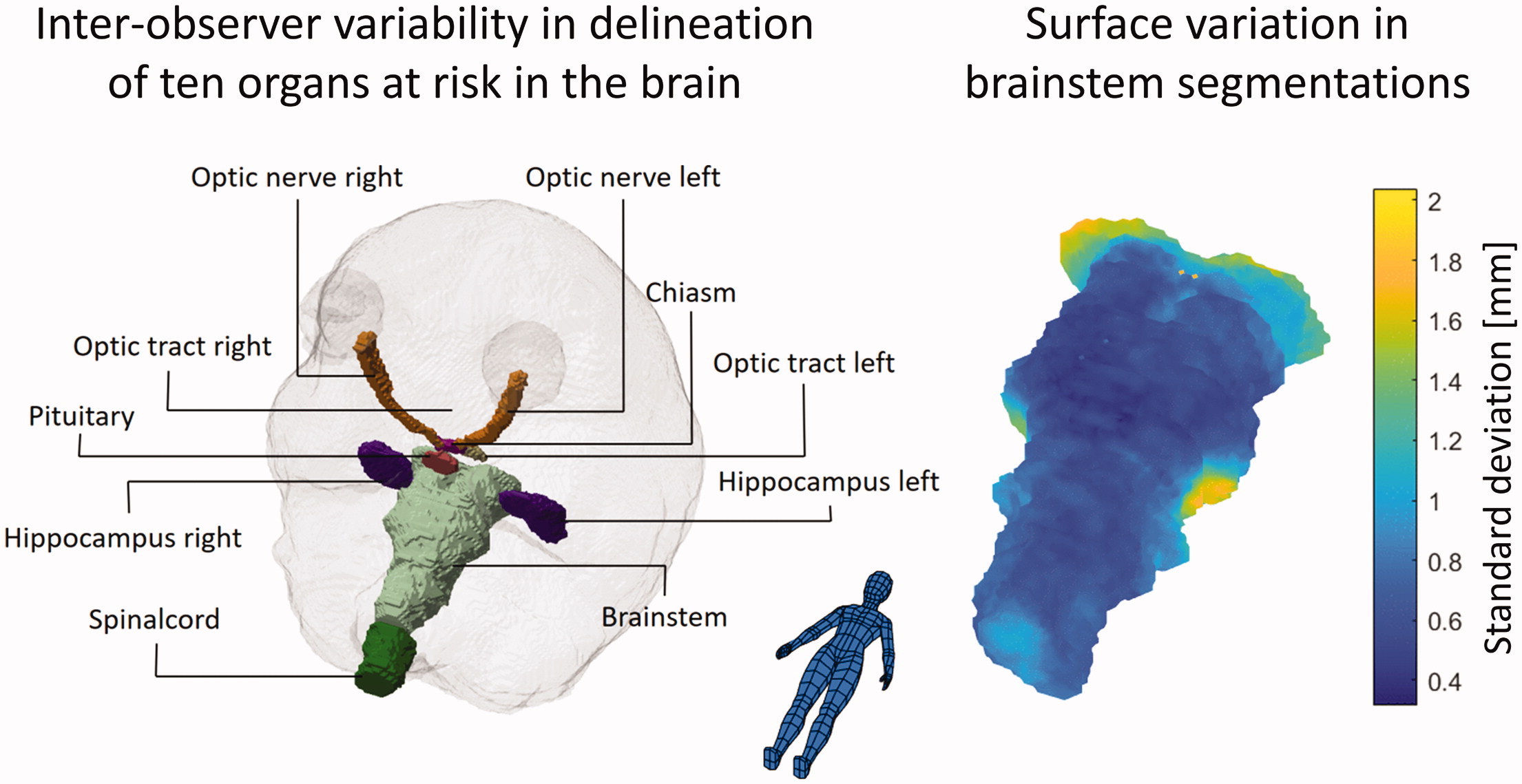
Graphical Abstract

Keywords:

• Organs at risk
• radiotherapy
• brain
• inter-observer variation
• auto-segmentation

Background

Various comprehensive guidelines for delineating normal tissue structures in the brain exists [1,2] and are inherently dependent on high quality and standardised magnetic resonance imaging (MRI) [3]. The implementation of these guidelines and evaluation of inter-observer variation has primarily been focussed on the clinical target (CTV) [4–6] and gross target volumes (GTV) [7,8]. Few studies have investigated delineation-variation of normal tissue structures in the brain. For the hippocampus, Bartel et al. [9] found an interclass correlation of 0.56 and 0.69 for the left and right hippocampus, respectively. The largest variations were seen in the posterior and anterior-medial hippocampal regions ranging from 1–2.5 mm standard deviation (SD). For brainstem, optic chiasm, eyes and optic nerves, Deeley et al. [10] found for eight expert physicians a relatively low mean Dice similarity coefficient (Dice) for the optic chiasm and optic nerves of 0.4 and 0.5, respectively. Mean Dice for the brainstem and eyes were considerably better being above 0.8 for both structures. In a later study by Deeley et al. [11] on the same patient cohort, it was noted that when only using a single expert, ground truth automatic segmentation of the small tubular structures performed poorly. However, in the context of several experts, they found that automatic segmentation performed no worse than the experts. They concluded that the inter-observer variance amongst the experts was similar to the automatic-to-expert variance, indicating that automatic systems are not inadequate but that these structures are inherently difficult to segment.

The study aimed to evaluate inter-observer variability amongst experts from the Danish Neuro Oncology Group (DNOG) participating in a workshop for relevant normal tissue structures in the brain. The results with multi-observer segmentations will be used as a benchmark for future auto-segmentation algorithms.

Material and methods

Study design

Ten oncologists (two participants from five different centres) were invited to participate in a two-day workshop with the task to delineate the following normal tissue structure for 13 randomly selected patients with brain cancer: optic tract left and right (L + R), optic nerve L + R, chiasm, spinal cord, brainstem, pituitary, hippocampus L + R and brain. Before the workshop, the oncologists were asked to delineate a single pilot patient that was distributed between the centres using the national radiotherapy plan bank, DcmCollab and the audit tool within [12]. The pilot patient was delineated according to the DNOG guidelines which have been adapted to the recommendation of Scoccianti et al. [1] for most organs except for the chiasm which is defined according to Brouwer et al. [13] to ensure consistency in OAR contouring relevant for both DNOG and the Danish Head and Neck Cancer Group (DAHANCA) [14]. The first point on the workshop agenda was to recapitulate delineations of this pilot patient and discuss differences between delineations. This was done to ensure a common understanding of the delineation guidelines before the subsequent individual delineation of patients.

The 13 patients were low-grade glioma patients previously treated with radiotherapy according to the DNOG guidelines. All patients had an x-ray treatment planning computed tomography (CT) scan of 2 or 3 mm slice thickness and a 1.5/3 T contrast-enhanced T1 weighted MRI with an approximately 1×1×1 mm resolution.

Data preparation and sanity cheques

Data were imported and analysed in MATLAB R2020b (version 9.9.0.1467703). Before any comparison was made between observers, sanity cheques were performed based on Matlab code in two ways: First, all contours consisting of separate non-connected volumes were identified and manually inspected (by a single person who had not participated in the segmentation work) for missing slices or major contouring errors – volumes were corrected if this could be done simply by deleting clearly wrongly delineated volumes. If the errors would have required re-delineation (e.g., a missing slice) the whole volume was deleted. Second, for all organs with laterality (left or right) the centre of mass of the organ relative to the centre of the image was calculated and any left/right naming errors were corrected. In all of the sanity cheques, only information from the single observer's segmentation under evaluation was used.

Comparison metrics

All contours were sampled to the resolution of the CT-scan in structure specific 3D masks. Based on these masks a range of metrics were computed: Dice, Jaccard index (Jaccard), Mean Surface Distance (MSD), Hausdorff distance (HD) and Hausdorff 95% distance (HD95). The Dice and Jaccard are both overlap metrics with values of one for perfect overlap and values of zero for no overlap. For two volumes (A and B) they are defined as: $$\mathrm{Dice}=\frac{2(A\cap B)}{A+B} \mathrm{Jaccard}=\frac{A\cap B}{A\cup B}$$

The MSD measures the average distance between the surface of two contours, and is defined by the one-sided Mean Surface Distance (msd): $$\mathit{msd}(A,B)=\frac{1}{N}\sum _{a\in A}\underset{b\in B}{\min }\parallel a-b\parallel \mathit{MSD}=\frac{1}{2}\left(\mathit{msd}(A,B)+\mathit{msd}(B,A)\right)$$ $\parallel a-b\parallel$ denotes the Euclidian distance between points a and b.

The HD measures the maximum of the shortest distances between two surfaces and is defined from the one-sided Hausdorff distance (hd): $$hd\mathrm{\hspace{0.17em}}(A,B)=\underset{a\in A}{\max }\underset{b\in B}{\min }\parallel a-b\parallel HD=\underset{}{\max }\left(hd(A,B)+hd(B,A)\right)$$

The HD95 is calculated similarly to the HD. However, instead of the max in the definition of the hd, the 95^th percentile is calculated.

For a given segmentation under evaluation, each metric was calculated pairwise between a specific segmentation and each of the remaining segmentations done by the other observers. The mean value of these formed the specific segmentations metric.

Surface mapping

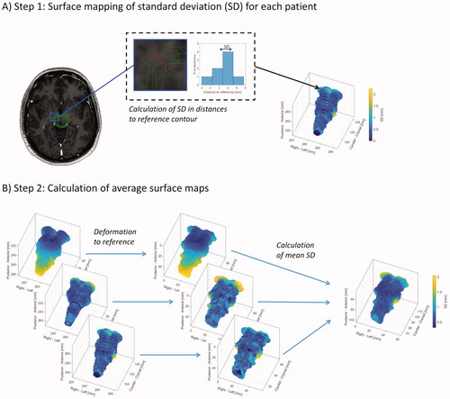
For all segmentation masks, surfaces were formed as triangulated meshes represented by faces and vertices. To visualise the spatial distribution and location of the inter-observer variability of these surfaces, the standard deviation (SD) of distances between observers was mapped in two steps, also illustrated in Figure 1: First, for each patient and OAR, a reference contour was selected as the contour with the lowest MSD (compared to the other observers). From each surface point (vertex) of this reference contour, the shortest distances to the remaining contours were calculated with sign (negative if inside the reference, positive if outside) and the SD of these distances was calculated. The surface of the reference contour was coloured by assigning the SD to the faces (interpolated from the corresponding vertices). Secondly, to get the individual patient surface maps of the inter-observer variation in the same coordinate system, affine image registration (linear transformation including translation, rotation, shear and scaling) was used on the binary masks of the reference contours from each patient to a specific patient selected arbitrarily as a reference patient. Based on this registration, the SD surfaces were registered to the coordinate system of the reference patient and the mean SD surface was calculated by finding the nearest surface point. These measures were used to visualise the inter-observer variations when averaged across all patients and observers.

Figure 1. Illustration of surface mapping of the inter-observer variation in segmentation. First, as illustrated in (A), the standard deviation (SD) in distance from the different segmentations to a specific segmentation selected as a reference were calculated for each patient and plotted on the surface of the reference contour. Secondly, as illustrated in (B), these patient-specific surfaces of the variation (SD), were transformed to a reference patient allowing the patient-specific surfaces to be plotted on the same surface and allowing for calculation of the SD across patients.

Results

A total of 968 contours were delineated across the 13 patients. On average eight (range six to nine) individual contour sets were made per patient. The Dice and MSD are shown in Figure 2 and all metrics tabulated in Table 1. Good agreement was found across all structures with a median MSD below 1 mm for most structures, with the chiasm performing the best with a median MSD of 0.45 mm. The Dice was primarily included to allow comparison to previously published studies and was also in this study found to be highly volume dependent. The brainstem (the largest structure) had the highest Dice value with a median of 0.89, although the median MSD with a value of 0.96 mm was slightly higher than the average value.

Figure 2. Boxplot of Dice similarity coefficient (Dice) and Mean Surface Distance (MSD) measures for the OAR in the brain. The individual data points indicate each observer’s patient-specific mean measure. Due to large variations in the caudal end of the spinal cord, metrics for the spinal cord are not shown in the boxplot but can be found in Table 1.

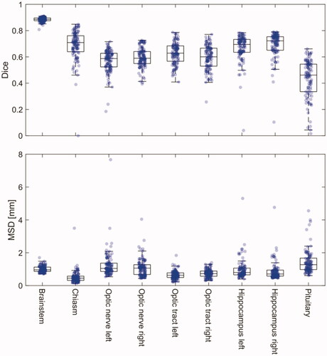
Table 1. Median volumes and comparison metrics with corresponding interquartile ranges shown in parentheses.

	Volume (cm^3)	Dice	Jaccard	MSD (mm)	HD (mm)	HD95 (mm)
Brainstem	27.2 (24.1–31.3)	0.89 (0.88–0.90)	0.79 (0.78–0.81)	1.0 (0.9–1.1)	6.6 (5.7–7.3)	3.3 (3.0–3.7)
Spinalcord	5.3 (2.6–7.5)	0.57 (0.44–0.60)	0.43 (0.30–0.47)	5.8 (4.9–8.4)	31.9 (27.0–43.5)	16.4 (14.2–21.8)
Chiasm	0.2 (0.1–0.3)	0.71 (0.64–0.76)	0.55 (0.48–0.62)	0.5 (0.3–0.6)	2.9 (2.1–3.7)	1.6 (1.3–2.0)
Optic nerve left	0.9 (0.6–1.1)	0.59 (0.52–0.63)	0.42 (0.36–0.46)	1.0 (0.9–1.4)	6.9 (5.1–8.2)	3.9 (3.2–4.5)
Optic nerve right	0.8 (0.7–1.1)	0.59 (0.55–0.64)	0.42 (0.38–0.48)	1.1 (0.7–1.3)	6.5 (4.1–7.7)	3.9 (2.3–4.7)
Optic tract left	0.2 (0.1–0.2)	0.63 (0.57–0.68)	0.46 (0.40–0.53)	0.6 (0.5–0.8)	3.4 (2.8–4.2)	2.1 (1.7–2.4)
Optic tract right	0.1 (0.1–0.2)	0.60 (0.53–0.67)	0.44 (0.37–0.51)	0.7 (0.6–0.9)	3.5 (2.9–3.9)	2.1 (1.8–2.5)
Hippocampus left	2.1 (1.7–2.5)	0.69 (0.63–0.73)	0.53 (0.47–0.58)	0.8 (0.7–1.1)	6.7 (6.0–8.2)	3.3 (2.8–3.9)
Hippocampus right	2.1 (1.7–2.5)	0.72 (0.65–0.75)	0.57 (0.49–0.61)	0.7 (0.6–0.9)	6.0 (5.3–7.5)	2.8 (2.6–3.5)
Pituitary	0.2 (0.2–0.3)	0.46 (0.34–0.54)	0.32 (0.22–0.40)	1.3 (1.0–1.7)	3.9 (3.5–4.9)	2.8 (2.3–3.4)

The metrics are as follows: the Dice similarity coefficient (Dice), Jaccard index (Jaccard), Mean Surface Distance (MSD), Hausdorff distance (HD) and Hausdorff 95% distance (HD95).

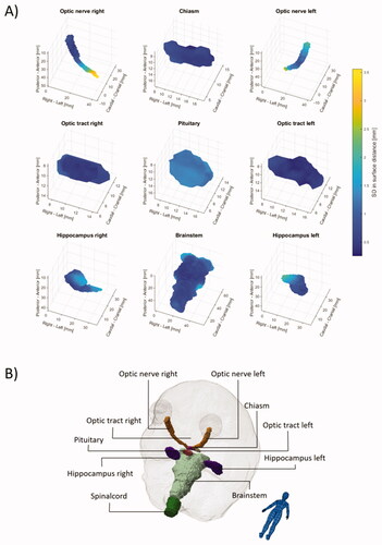
The mean SD surfaces are shown in Figure 3 with individual plots shown in the Supplementary figures 1–10. Several of the spinal cord delineations did not include the caudal part, which is contrary to the guidelines. This resulted in large and irrelevant inter-observer variations, hence metrics are omitted in Figures 2 and 3, but are listed in Table 1.

Figure 3. Surface maps of the inter-observer variability given as the mean standard deviation (SD) across the 13 patients are shown in (A). Anatomical directions are illustrated in (B). Due to large variation in the caudal end of the spinal cord maps for the spinal cord is not shown. Individual animated maps can be found in Supplementary figures 1–10.

Discussion

Inter-observer variability in the segmentation of organs at risk in the brain by experts from the Danish radiotherapy centres was, compared to prior work, in general, low and the segmentations were of high consistency. The variability measured in our study represents a best-case scenario; the observers did the segmentations following a review and discussion of present guidelines, and in a clinical setting the variability would be expected to be higher. Ongoing quality assurance of segmentations across centres is likely needed to maintain both the inter and intra-centre consistency. In the context of benchmark for future auto segmentation validation, this data will set a high bar for the performance of these algorithms.

Bartel et al. evaluated the multi-centre inter-observer variability in the delineation of the hippocampi by seven observers and reported a generalised conformity index, which is a similar metric to the Jaccard index reported in this study. They found a generalised conformity index of 0.56 and 0.69 for the left and right hippocampus compared to a slightly worse median Jaccard of 0.53 and 0.57 respectively in this study. Bartel et al. performed surface mapping of the SD with a very similar approach, however, without calculating the mean SD surface as presented in this study. Their individual patient maps were, however, similar with a maximum SD of approximately 2 mm, predominantly at the anterior and posterior regions.

Compared to the study by Deeley et al., who reported the inter-observer variability by eight observers’ segmentation of organs at risk in the brain, the variability was lower in our study. They found mean Dice values of the brainstem, chiasm and optic nerves (as one structure) of 0.825, 0.392 and 0.499 compared to 0.89, 0.71 and 0.59 (for both left and right optic nerves) in this study. While both CT and T1 MRI were available in their study, other factors might be the cause of the larger variability; no contrast was apparently used, their patients were all selected as high-grade glioma with relative large tumours close to the delineated organs at risk and the observers in our study did their segmentations immediately after review and discussion of present guidelines.

A wide range of metrics is used for comparing segmentations [15,16]. In this study, several metrics were used to allow comparison with published studies. Both overlap metrics (Dice and Jaccard), as well as metrics related to the distance between surfaces (MSD, HD, HD95), were used. While the overlap metrics are well defined and relatively easy to calculate, they carry little information in themself. The volume dependency of these metrics is well known and also present in our study with larger volumes having larger overlap metrics.

The surface mapping of the SD and the generation of a mean SD on a representative surface revealed that for several organs sub-regions of higher uncertainty were present. In addition to the hippocampi as described above, this was especially notable for the brainstem and the optic nerves. For the brainstem, the SD at the cranial end and at the middle cerebellar peduncles were 1.5–2 mm compared to an SD of less than 1 mm for the rest of the surface. The higher variance in these regions is expected due to the lack of clear anatomical borders and tissue contrast. For the optic nerves, the variation was largest at the posterior end with an SD of 2.5–3.5 mm compared to an SD of less than 1 mm at the anterior end, presumably connected to a slightly different approach in the transition from the optical nerve to the chiasm. These localised regions of larger variability show the limitations of summarising metrics such as the MSD and HD. Therefore, when evaluating automatic segmentation, a comparison of any deviation between manual and automatic segmentation with inter-observer variations could preferably also be done based on the surface mapping to identify local areas of discrepancies.

In our study, neither the impact of inter-observer variability on measured dose to OAR nor the impact on the radiotherapy planning was investigated. While variation in a measured dose, i.e., the difference in dose due to differences in delineations but with the same dose distribution, is clinically relevant, the measured variability is highly dependent on the dose distribution. For example, looking at the mean dose to a given organ, the more the local dose at a surface point differ from the mean dose to the same organ, the higher the impact of the spatial variation at that specific point [17]. An impact on treatment, i.e., where changes in delineations of OAR would lead to different treatment plans, is most likely to happen for structures considered critical serial OAR with max/near max dose constraints. The brainstem and optical nerves are both such OAR and the surface regions with systematically higher variation observed in our study could be considered in the treatment planning process. This could be done either by careful evaluation of the segmentation when target regions are located near these regions and/or by applying heterogeneous PRV margins.

In Denmark, patients are referred to proton therapy based on a treatment plan comparison between photons and protons. The consistent segmentation shown in this study will allow a consistent comparison in dose to OAR across centres and observers. It will also allow for better normal tissue complication (NTCP) models to be developed and validated, as the variances and hence the dose-response relationship has less variance [18].

In the future, these findings and data will be used as a benchmark for automatic segmentation methods, where the inter-observer variability can be compared to any potential differences observed between automatic and manual segmentations. In a first step, such an evaluation can be done in a separate dataset where any observed differences between automatic and manual segmentations can be compared to the inter-observer variabilities observed in the present study. If a given automatic segmentation algorithm is determined to be of sufficient precision and thereby final, it can be tested directly on the data in this study. Such a final evaluation should only be performed once for a given algorithm to avoid overfitting and the results should be published. The authors are open to collaboration on evaluating automatic segmentation algorithms.

Conclusion

The observed variances in the T1 MRI-guided contours of OARs in the brain were low and consistent with a mean surface distance typically lower than 1 mm. For some organs, surface mapping did reveal sub-regions of higher uncertainty with a mean SD of 2–3mm. The data will be used as validation data set for auto-segmentation algorithms for use within the Danish Comprehensive Cancer Centre – Radiotherapy and potential collaborators.

Disclosure statement

No potential conflict of interest was reported by the author(s).

Additional information

Funding

The current study and workshop were supported by DCCC Radiotherapy – The Danish National Research Centre for Radiotherapy, Danish Cancer Society [grant no. R191-A11526] and Danish Comprehensive Cancer Centre and the Region of Southern Denmark – BRAIN project.

References

- Scoccianti S, Detti B, Gadda D, et al. Organs at risk in the brain and their dose-constraints in adults and in children: a radiation oncologist’s guide for delineation in everyday practice. Radiother Oncol. 2015;114(2):230–238.
- Eekers DB, In’t Ven L, Roelofs E, et al. The EPTN consensus-based atlas for CT- and MR-based contouring in neuro-oncology. Radiother Oncol. 2018;128(1):37–43.
- Ellingson BM, Bendszus M, Boxerman J, et al. Consensus recommendations for a standardized brain tumor imaging protocol in clinical trials. Neuro Oncol. 2015;17(9):1188–1198.
- Jansen EPM, Dewit LGH, van Herk M, et al. Target volumes in radiotherapy for high-grade malignant glioma of the brain. Radiother Oncol. 2000;56(2):151–156.
- Soliman H, Ruschin M, Angelov L, et al. Consensus contouring guidelines for postoperative completely resected cavity stereotactic radiosurgery for brain metastases. Int J Radiat Oncol. 2018;100(2):436–442.
- Kruser TJ, Bosch WR, Badiyan SN, et al. NRG brain tumor specialists consensus guidelines for glioblastoma contouring. J Neurooncol. 2019;143(1):157–166.
- Crowe EM, Alderson W, Rossiter J, et al. Expertise affects inter-observer agreement at peripheral locations within a brain tumor. Front Psychol. 2017; 8:1628. [cited 2021 May 3]. Available from: https://www.ncbi.nlm.nih.gov/pmc/articles/PMC5611391/
- Weltens C, Menten J, Feron M, et al. Interobserver variations in gross tumor volume delineation of brain tumors on computed tomography and impact of magnetic resonance imaging. Radiother Oncol. 2001;60(1):49–59.
- Bartel F, van Herk M, Vrenken H, et al. Inter-observer variation of hippocampus delineation in hippocampal avoidance prophylactic cranial irradiation. Clin Transl Oncol. 2019;21(2):178–186.
- Deeley MA, Chen A, Datteri R, et al. Comparison of manual and automatic segmentation methods for brain structures in the presence of space-occupying lesions: a multi-expert study. Phys Med Biol. 2011;56(14):4557–4577.
- Deeley M, Chen A, Datteri R, et al. Segmentation editing improves efficiency while reducing inter-expert variation and maintaining accuracy for normal brain tissues in the presence of space-occupying lesions. Phys Med Biol. 2013;58(12):4071–4097.
- Brink C, Lorenzen EL, Krogh SL, et al. DBCG hypo trial validation of radiotherapy parameters from a national data bank versus manual reporting. Acta Oncol. 2018;57(1):107–112.
- Brouwer CL, Steenbakkers RJHM, Bourhis J, et al. CT-based delineation of organs at risk in the head and neck region: DAHANCA, EORTC, GORTEC, HKNPCSG, NCIC CTG, NCRI, NRG Oncology and TROG consensus guidelines. Radiother Oncol. 2015;117(1):83–90.
- Jensen K, Friborg J, Hansen CR, et al. The Danish Head and Neck Cancer Group (DAHANCA) 2020 radiotherapy guidelines. Radiother Oncol. 2020;151:149–151.
- Jameson MG, Holloway LC, Vial PJ, et al. A review of methods of analysis in contouring studies for radiation oncology: techniques of contour comparison. J Med Imaging Radiat Oncol. 2010;54(5):401–410.
- Vinod SK, Jameson MG, Min M, et al. Uncertainties in volume delineation in radiation oncology: a systematic review and recommendations for future studies. Radiother Oncol. 2016;121(2):169–179.
- Lorenzen EL, Ewertz M, Brink C. Automatic segmentation of the heart in radiotherapy for breast cancer. Acta Oncol. 2014;53(10):1366–1372.
- Hansen CR, Friborg J, Jensen K, et al. NTCP model validation method for DAHANCA patient selection of protons versus photons in head and neck cancer radiotherapy. Acta Oncol. 2019;58(10):1410–1415.