Computer modelling of burden distribution in the blast furnace equipped by a bell-less top charging system

ABSTRACT

This article describes the simulation method for layering the components of the charge in the blast furnace, including the particle size distribution and gas flow distribution of bell-less top charging systems in blast furnaces. The Burden Distribution application, which simulates the charge in blast furnaces operated by the company Třinecké železárny (ironworks) to optimize the production of pig iron, applied this simulation method. Based on the parabolic trajectory of the material falling from the tilting chute of the bell-less top charging system, the method is calculating the profile of individual charge layers. The material forms after impact according to known angles of repose, segregating into individual granulometric size fractions. The data incorporated into the simulation enables the estimation of charge and gas flow distribution along the radius of the blast furnace shaft. The article presents the used mathematical models and equations, including algorithms of the simulation.

KEYWORDS:

• Blast furnace
• bell-less top
• burden distribution
• stack profile
• segregation
• algorithm
• application
• computer simulation

Introduction

The profile of the individual blast furnace charge components determines the reducing gas flow distribution and thus the performance and energetic parameters of the operation of the blast furnace and consequently the production of pig iron. Technologists have therefore been striving to attain information about gas flow and charge distribution. A bell-less top charging system is a useful tool for controlling both these flows. We can measure the effects of changes in the charging program, which consist of step-by-step changing the chute inclination during rotation both directly and indirectly. Indirect information includes temperature distribution on the perimeter of the charging system and in the gas pipelines, whereas profilometers can obtain direct information. Another option is to conduct mathematical simulations, which makes it possible to gain detailed information with minimal costs.

This article focuses on a method for calculating a simulated model of the burden layer profile, including granulometric size distribution based on measurements of individual parameters and a simulation calculation. The well-researched parabolic falling trajectory of the burden leaving the chute of the bell-less top charging system is the basis of this model. The angle of the chute and the velocity of the burden leaving the tip of the chute to define the trajectory.

After the material falls, it forms into a shape according to known angles of repose. The granular material segregates into the individual granulometric size fractions along the shaft radius of the blast furnace based on experimental estimation. The segregation of granular material means that larger pieces move further from the place of impact, while smaller pieces stay near the place of impact. An approximate differential equation describes granulometric segregation. Many experimenters explore the behaviour of gas flow through charges. There are even parameters available describing the dependence of pressure loss on the volume flow square for materials with known granulometric size spectra. All this data incorporates into the simulation calculation, which makes it possible to estimate the charge flow and gas distribution along the radius of the blast furnace stack.

Burden distribution simulation model

The model simulates the burden distribution on the radius of the blast furnace shaft. During charging, the chute of the bell-less top charging system rotates and gradually changes the angle of inclination $\alpha$, so that the individual placements of iron ore or sinter, coke and additives like for example limestone could be checked along the shaft radius. In simple terms, we can assume that separate charges flow along the falling trajectory (Figure 1).

Figure 1. Schematic diagram of the principle of the burden distribution model.

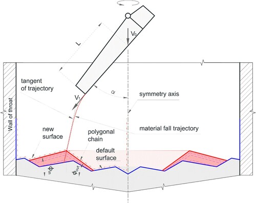
The velocity of the burden into the chute and the chute angle determine the material falling trajectory. Equation (1) describes the velocity of the burden at the tip of the chute calculation [1]. (1) $v_1=\sqrt[2]{\begin{array}{rl}& v_0^2{\cos }^2\left(\alpha \right)+{\omega }^2{L}^2\sin \left(\alpha \right)\left(\sin \alpha +\mu \cos \alpha \right)\\ & +2gL\left(\cos \alpha -\mu \sin \alpha \right)\end{array}}$(1) where $v_0$ is the vertical velocity of the particles on impact with the chute [m s⁻¹], $L$ is the chute distance travelled [m], $\omega$ is the chute rotation speed [rad s⁻¹], $\mu$is the shear friction factor, $g$ is the acceleration of gravity [m s⁻²], and $\alpha$ is the angle of inclination of the chute compared to the axis of symmetry [rad].

Equations (2) and (3) describe the falling curve [1]. (2) $r\left(t\right)=L\sin \alpha +\left(v_1\sin \alpha \right)t$(2) (3) $y\left(t\right)=y_0-L\cos \alpha -{\displaystyle \frac{g{t}^2}{2}-\left(v_1\cos \alpha \right)t}$(3)

After expressing time $t$ from Equation (2) and substituting it into Equation (3) we get an Equation (4) of the falling curve. (4) $y=-{\displaystyle \frac{g}{2v_1^2{\sin }^2\alpha }{r}^2+{\displaystyle \frac{gL-v_1^2\cos \alpha }{v_1^2\sin \alpha }r+y_0-{\displaystyle \frac{g{L}^2}{2v_1^2}}}}$(4) where $r$ represents the distance of the falling trajectory from the central axis, $y$ is the vertical coordinate of the falling trajectory, $v_0$ is the vertical velocity of the particles on impact with the chute [m s⁻¹]. The $L$ is the chute distance travelled [m], $\omega$ is the chute rotation speed [rad s⁻¹], $\mu$is the shear friction factor, $g$ is the acceleration of gravity [m s⁻²], $\alpha$ is the chute inclination angle compared to the axis of symmetry [rad], $y_0$ is the vertical coordinate of the beginning of the chute.

Randomizing the velocity of the burden leaving the chute tip models the scatter of the charge on the impacting stockline surface. The volume of the charge falling into one annulus (a region bounded by two concentric circles) divides into virtual sub-charges with assigned various velocities for the scatter parameter. These sub-charges then move along various falling curves. This method brings the model closer to realistic conditions.

The substitution by two or more lines, a cubic curve, or the Gaussian curve builds the burden profile mathematical model [2–5]. It is most often represented by two lines, which are beneath the material angles of repose and intersect on the falling trajectory [1,6–8]. A polygonal chain gives the surface and interface between the burden components, which is composed of line segments passing through a sequence of points $P_i\left(r_i,y_i\right)$ called its vertices. Line Equation (5) describes the surface of the charge. (5) $p_i\left(r\right)=a_{i}r+b_i,i=1,2,\dots ,n$(5)

In solving Equation (6), we find the intersection point of the falling curve with the polygonal chain representing the surface of the charge (including the furnace walls) determines the points of impact$I\left(r_I,y_I\right)$. (6) $0=-{\displaystyle \frac{g}{2v_1^2{\sin }^2\alpha }{r}_I^2+{\displaystyle \frac{gL-v_1^2\left(\cos \alpha -a_i\sin \alpha \right)}{v_1^2\sin \alpha }{r}_I+y_0-{\displaystyle \frac{g{L}^2}{2v_1^2}-b_i}}}$(6)

The maximum angle formed between the surface line of the cone formed by the charge and the horizontal plane represents the angle of repose. Generally, the repose angle depends on the properties of the material, like its density, size and grain shape, and the coefficient of friction of the material [9]. When the burden settles, its angle of repose varies concerning the axis of symmetry ${\phi }_{\mathrm{i}\mathrm{n}}$ (inner angle) from the angle in the direction of the wall ${\phi }_{\mathrm{o}\mathrm{u}\mathrm{t}}$ (outer angle). The repose angle in the direction of the wall is significantly smaller. Equations (7) and (8) express the nominal repose angles [8]. (7) $se{t}_{\mathrm{i}\mathrm{n}}=se{t}_{\mathrm{m}\mathrm{a}\mathrm{x}}C{\displaystyle \frac{d^{0.05}}{4F_S^{0.05}}}$(7) (8) $se{t}_{\mathrm{o}\mathrm{u}\mathrm{t}}=se{t}_{\mathrm{i}\mathrm{n}}{\displaystyle \frac{R-r_I^{1.4}}{5.8}}$(8) where $se{t}_{\mathrm{m}\mathrm{a}\mathrm{x}}$ is the maximum angle of repose [deg], $C$ is a constant, $d$ is the diameter of the particle [m], $F_S$ is the shape dimensionless factor [–], $R$ is the radius of the throat [m], $r_I$ is the distance [m] from the symmetry axis to the intersection point of the trajectory and the burden surface.

The falling trajectory, i.e. the chute angle, also affects the repose angle. In practice, angles of repose are determined experimentally with the help of scaled-down blast furnace models [8]. Then it is possible to connect individual repose angles with each position of the chute. Another option is to correct repose angles according to the deviation of the tangent angle $t_I\left(r\right)$ to the falling trajectory at the point of impact. Equation (9) describes the tangent to the trajectory at the point of intersection. (9) $t_I\left(r\right)=m_{I}r+n_I=-\left(g{\displaystyle \frac{r_I-l\sin \alpha }{{\left(v_{\mathrm{o}\mathrm{u}\mathrm{t}}\sin \alpha \right)}^2}+\mathrm{c}\mathrm{o}\mathrm{t}\mathrm{n}\left(\alpha \right)}\right)r+\left[g{\displaystyle \frac{r_I-l\sin \alpha }{{\left(v_{\mathrm{o}\mathrm{u}\mathrm{t}}\sin \alpha \right)}^2}-\mathrm{c}\mathrm{o}\mathrm{t}\mathrm{n}\left(\alpha \right)}\right]r_I+y_I$(9) (10) $m_I=-g{\displaystyle \frac{r_I-L\sin \alpha }{{\left(v_1\sin \alpha \right)}^2}-\mathrm{c}\mathrm{o}\mathrm{t}\mathrm{n}\left(\alpha \right)}$(10)

The slope of the $m_I$ tangent to the falling trajectory at the point of impact $t_I\left(r\right)$ is used to determine the difference between the angle of incidence and the vertical axis, which is multiplied by the correction constants $c_{\mathrm{i}\mathrm{n}}$, $c_{\mathrm{o}\mathrm{u}\mathrm{t}}$ for a given type of angle. The resulting values are then subtracted from the nominal repose angles $se{t}_{\mathrm{i}\mathrm{n}}$, $se{t}_{\mathrm{o}\mathrm{u}\mathrm{t}}$. (11) ${\phi }_{\mathrm{i}\mathrm{n}}=se{t}_{\mathrm{i}\mathrm{n}}+\left({\displaystyle \frac{\pi }{2}+{\tan }^{-1}{m}_I}\right)c_{\mathrm{i}\mathrm{n}}$(11) (12) ${\phi }_{\mathrm{o}\mathrm{u}\mathrm{t}}=\left({\displaystyle \frac{\pi }{2}+{\tan }^{-1}{m}_I}\right)c_{\mathrm{o}\mathrm{u}\mathrm{t}}-se{t}_{\mathrm{o}\mathrm{u}\mathrm{t}}$(12)

Charge layering algorithm

First, we must find the nearest point of the polygon chain of the charged surface (at the same or higher height) $P_j\left(r_j,y_j\right)$ to the intersection point$I\left(r_I;y_I\right)$. Depending on whether the found point is in the direction of the axis of symmetry or towards the charging system wall, a line $k\left(r\right)$ is run through the point under the inner ${\phi }_{\mathrm{i}\mathrm{n}}$ or the outer repose angle ${\phi }_{\mathrm{o}\mathrm{u}\mathrm{t}}$. Subsequently, the algorithm inserts a line through the intersection point of this line $K\left(r_K,y_K\right)$ with the tangent to the trajectory $t_I\left(r\right)$ under the second repose angle. (13) $k\left(r\right)=\{\begin{array}{c}\begin{array}{c}\tan \left({\phi }_{\mathrm{i}\mathrm{n}}\right)r+y_j-\tan \left({\phi }_{\mathrm{i}\mathrm{n}}\right)r_j\end{array},r_j\le r_I\\ \begin{array}{c}\tan \left({\phi }_{\mathrm{i}\mathrm{n}}\right)r+y_K-\tan \left({\phi }_{\mathrm{i}\mathrm{n}}\right)r_K\end{array},r_j>r_I\end{array}$(13) (14) $l\left(r\right)=\{\begin{array}{c}\tan \left({\phi }_{\mathrm{o}\mathrm{u}\mathrm{t}}\right)r+y_K-\tan \left({\phi }_{\mathrm{o}\mathrm{u}\mathrm{t}}\right)r_K,r_j\le r_I\\ \tan \left({\phi }_{\mathrm{o}\mathrm{u}\mathrm{t}}\right)r+y_j-\tan \left({\phi }_{\mathrm{o}\mathrm{u}\mathrm{t}}\right)r_j,r_j>r_I\end{array}$(14)

The intersection point of this second line with the polygon chain given by the vertices $p_i\left(r\right)$determines the second peripheral point of the surface of the added increment $L\left(r_L,y_L\right)$. The points$L\left(r_L,y_L\right)$, $K\left(r_K,y_K\right)$, $P_j\left(r_j,y_j\right)$ together with points$P_i\left(r_i,y_i\right),i=1,2,\dots ,n$ that are not below the triangle $L$, $K$, $P_j$ form a new surface resulting in the polygon chain containing the vertices $p\left(r\right)$. (15) $p\left(r\right)=\{\begin{array}{c}{a}_{i}r+b_i,r〈\mathrm{m}\mathrm{i}\mathrm{n}\left(r_L,r_j\right)\cap r〉\mathrm{m}\mathrm{a}\mathrm{x}\left(r_L,r_j\right),\\ i=1,2,\dots ,n\\ k\left(r\right),r\ge \mathrm{m}\mathrm{i}\mathrm{n}\left(r_L,r_j\right)\cup r<r_I\\ l\left(r\right),r\le \mathrm{m}\mathrm{a}\mathrm{x}\left(r_L,r_j\right)\cup r\ge r_I\end{array}$(15)

At the same time points $L\left(r_L,y_L\right)$, $K\left(r_K,y_K\right)$, $P_j\left(r_j,y_j\right)$ and the points$P_i\left(r_i,y_i\right),i=1,2,\dots ,n$ located below the triangle $L$, $K$, $P_j$ form the vertices of a polygonal chain $m\left(r\right)$. (16) $m\left(r\right)=\{\begin{array}{c}{a}_{i}r+b_i,r>\mathrm{m}\mathrm{i}\mathrm{n}\left(r_L,r_j\right)\cup r<\mathrm{m}\mathrm{a}\mathrm{x}\left(r_L,r_j\right),\\ i=1,2,\dots ,n\\ k\left(r\right),r\ge \mathrm{m}\mathrm{i}\mathrm{n}\left(r_L,r_j\right)\cup r<r_I\\ l\left(r\right),r\le \mathrm{m}\mathrm{a}\mathrm{x}\left(r_L,r_j\right)\cup r\ge r_I\end{array}$(16)

The polygonal chain $m\left(r\right)$ with vertices $M_i\left(r_i,y_i\right)$ represents the cross-section of the rotating body of the dumped charge. The area of a polynomial multiplied with the path length of its centre of gravity (Guldin’s rule) calculates the volume of a body. The algorithm calculates the additional individual triangles, which the polygonal chain is based on. The centre of gravity of the triangles is in a third of the median. (17) $\begin{array}{rl}V& =2\pi \sum _{i=3}^n[\left(r_1-r_{i-1}\right){\displaystyle \frac{y_1+y_{i-1}}{2}+\left(r_{i-1}-r_i\right){\displaystyle \frac{y_{i-1}+y_i}{2}}}\\ & +\left(r_i-r_1\right){\displaystyle \frac{y_i+y_1}{2}]{\displaystyle \frac{r_1+r_{i-1}+r_i}{3}}}\end{array}$(17)

For the list of points indexed from zero, we can write the algorithm of the calculation of the volume in the language C# in the following manner.

Table

static double V(List<POINT> M)

{

double S, DV = 0;

for (int i=2; i < M.Count; i++)

{

S = (M[0].r - M[i-1].r)*(M[0].y + M[i-1].y);

S += (M[i-1].r - M[i].r)*(M[i-1].y + M[i].y);

S += (M[i].r - M[0].r)*(M[i].y + M[0].y);

DV += S*(M[0].r + M[i-1].r + M[i].r);

}

return Math.PI*DV/3;

}

It is necessary to compare the calculated volume $V$ with the to-be-dumped volume $U_k$ along the given trajectory. In the first run, the remainder $V_R$ is set as the required volume $U_k$. The algorithm performs iterations with the updated surface if the ratio of the rest of the required volume is greater than the permissible error ${ϵ}_V$ (see Equation (18)), while the calculated point $K\left(r_K,y_K\right)$ becomes the new point of impact $I\left(r_I,y_I\right)$ and the charge volume reduces by the amount of the calculated volume $V_R:=V_R-V$. (18) ${\displaystyle \frac{V_R-V}{U_k}\le {ϵ}_V}$(18)

If the calculated volume $V$ in the last cycle is greater than the charge volume remainder $V_R$, the algorithm keeps the last surface, and measure the straight distance $l_{IK}$ between the intersection point $I\left(r_I,y_I\right)$ and the calculated point $K\left(r_K,y_K\right)$. The distance $l_{IK}$ has also a negative sign assigned. Then the numerical cycle for searching for $K\left(r_K,y_K\right)$ starts, while it is valid that the calculated volume is equal to the remainder within the given tolerance. The algorithm within the cycle first halves the distance $l_{IK}$, and then the point $K\left(r_K,y_K\right)$ moves along the tangent by a distance of $l_{IK}$ below or above the original position, depending on its sign. This point is then interlaced with the lines $k\left(r\right)$ and $l\left(r\right)$. (19) $k\left(r\right)=\tan \left({\phi }_{\mathrm{i}\mathrm{n}}\right)r+y_K-\tan \left({\phi }_{\mathrm{i}\mathrm{n}}\right)r_K$(19) (20) $l\left(r\right)=\tan \left({\phi }_{\mathrm{o}\mathrm{u}\mathrm{t}}\right)r+y_K-\tan \left({\phi }_{\mathrm{o}\mathrm{u}\mathrm{t}}\right)r_K$(20)

Then the intersection points $L\left(r_L,y_L\right)$, $P\left(r_P,y_P\right)$ of $l\left(r\right)$ and $k\left(r\right)$ are defined by the polygonal chain vertices $p_i\left(r\right)$, where $p_i$ is a vertical coordinate and $r$ is the distance from the blast furnace axis. By adding points $P_i\left(r_i,y_i\right),i=1,2,\dots ,n$ located below the triangle $L$, $K$, $P$, a polygonal chain is formed by the points $m\left(r\right)$, and the volume $V$ of the rotating body is calculated. The volume is compared with the remaining to be added $U_R$ volume, where the sign of the difference between the remaining volume and the calculated volume determines the current sign of the calculated distance $l_{IK}$. The cycle repeats until the ratio of the remainder to the required volume is greater than the allowable tolerance. (21) ${\displaystyle \frac{\left|V_R-V\right|}{U_k}\le {ϵ}_V}$(21)

After a suitable peak $K\left(r_K,y_K\right)$ is found, the polygon chain vertices of the surface updates to $p\left(r\right)$.

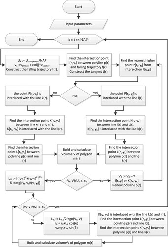
The described algorithm shown in Figure 2 repeats for all determined charge trajectories. When all charges process all set positions of the chute, the resulting polygon chain vertices are stored as a representation of the surface of the dump layer.

Figure 2. Flow chart of the charging algorithm of one chute position.

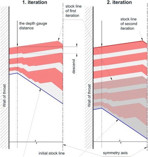
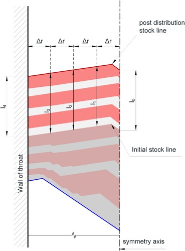
After every completed layer, the charge decreases by the height of the last layer at the location of measurement with a depth gauge. This ensures that the height of the material is always the same at the location of measurement (see Figure 3). Another option is to calculate the reduction based on the volume of the dumped layer, for example, using Equation (25) [10].

Figure 3. Burden descend during two interactions of the charging components algorithm.

The entire algorithm repeats for all groups and materials in the group (see Figure 4). Repeating calculations of the profile with the corresponding descent of the burden compensates for the fact of unknown initial burden profile.

Figure 4. Flow chart of the charging algorithm.

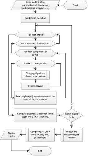
The calculation of one completed charging program iterates to the point when the difference of the initial and final profile is smaller than the permissible error ${ϵ}_{SL}$ (see Figure 5 and Equation (22)). The error value ${ϵ}_{SL}$ is usually set to 0.01 m. The charging program represents the sequence of chute inclinations for individual charge components, including their repetition. (22) ${\displaystyle \frac{1}{n}\sum _{i=1}^n\left|l_i-{\displaystyle \frac{1}{n}\sum _{j=1}^n{l}_j}\right|\le {ϵ}_{SL}}$(22)

Figure 5. Principle of calculating the difference between the initial and final stockline.

Burden descent in stack

The burden descent in the stack of the blast furnace depends on the angle of the walls and the dimensions of the throat (see Figure 6). The basic model calculates the same vertical descent velocity, where every vertex of the polygonal chain moves by the same distance $\mathrm{\Delta }y$, provided that the volume of the layer $U_C$ before and after the descent $U_C^{\mathrm{\prime }}$ is the same [10]. (23) $\mathrm{\Delta }{y}_i=y_i-y_i^{\mathrm{\prime }}=\mathrm{\Delta }{y}_{i-1},i=2,\dots n$(23) (24) $U_C=U_C^{\mathrm{\prime }}$(24)

Figure 6. The illustration of the layer descends in the throat and the stack part of the blast furnace.

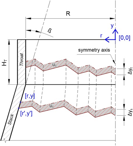
We can calculate the descent $\mathrm{\Delta }{y}_T$ of the burden in the cylindrical parts (Throat, Stack, and Barrel) of the blast furnace by Equation (25). (25) $\mathrm{\Delta }{y}_T={\displaystyle \frac{U_C}{\pi R^2}}$(25) where $U_C$ is the volume of the component layer, and $R$ is the radius of the cylindrical part of the blast furnace. The radii of the individual vertices of the polygonal chain remain the same. That is, we can calculate coordinates $y_i^{\mathrm{\prime }}$ and $r_i^{\mathrm{\prime }}$ of all points of the vertices of the polygon chain after descending in the cylindrical parts of the blast furnace by Equations (26) and (27). (26) $y_i^{\mathrm{\prime }}=y_i-{\displaystyle \frac{U_C}{\pi R^2}}$(26) (27) $r_i^{\mathrm{\prime }}=r_i$(27)

If there is a layer over the entire diameter of the furnace, then we can calculate the descent $\mathrm{\Delta }{y}_s$ in the conical parts (Stack, Bosh) of the blast furnace by Equation (28). (28) $\mathrm{\Delta }{y}_s=y-{\displaystyle \frac{R}{\tan \text{β}}+H_T+\sqrt[3]{{\left({\displaystyle \frac{R}{\tan \text{β}}-H_T-y}\right)}^3+{\displaystyle \frac{3U_C}{\pi {\tan }^2\text{β}}}}}$(28) where $y$ is the coordinate of the point of the original vertices of the polygon chain on the furnace wall before the descent, $H_T$ is the height of the throat, $R$ is the radius of the throat, $\text{β}$ is the wall inclination angle, $U_C$ is the volume of the layer. Therefore, we can calculate the coordinate $y_i^{\mathrm{\prime }}$ of the points of the vertices of the polygon chain after descending in the conical parts of the blast furnace by Equation (29). In addition, we proportionally adjust the radii of the individual vertices of the polygon chain by Equation (30) [10]. (29) $y_i^{\mathrm{\prime }}={\displaystyle \frac{R}{\tan \text{β}}-H_T-\sqrt[3]{{\left({\displaystyle \frac{R}{\tan \text{β}}-H_T-y_i}\right)}^3+{\displaystyle \frac{3U_C}{\pi {\tan }^2\text{β}}}}}$(29) (30) $r_i^{\mathrm{\prime }}=r_i{\displaystyle \frac{{\displaystyle \frac{R}{\tan \text{β}}-H_T-{y^{\mathrm{\prime }}}_i}}{{\displaystyle \frac{R}{\tan \text{β}}-H_T-y_i}}}$(30)

We can also solve the descent under the described conditions numerically. First, we approximately calculate the descent with Equations (25) and (26), and then we adjust the descent value $y_i$ until the new volume corresponds to the original volume. In the more advanced modelling methods, we calculate the descent with the burden descent speed variable [10].

Modelling the granulometric size distribution of the burden after impact

Many papers deal with the topic of size segregation of particle mixture in conical pile formation [6,11,12]. Experiments have shown that an approximation model can be used to describe segregation, according to which the change in the concentration of the granulometric size fraction c relative to the distance of the point of impact $x$ is proportional to its concentration and the remainder of the concentration to 1 (meaning 100%) [6]. We designate the proportionality factor by coefficient $\alpha$ in the following differential Equation (31). (31) ${\displaystyle \frac{dc}{dx}=-\alpha c\left(1-c\right)}$(31)

In solving this equation, we find the relation $c\left(x\right)$ between the change of the concentration of the granulometric size fraction and the distance of the point of impact (see Equation (32)). (32) $c\left(x\right)={\displaystyle \frac{1}{1+b{e}^{\alpha x}}}$(32) where we calculate the parameter $b$ according to Equation (33). (33) $b={\displaystyle \frac{1}{c\left(0\right)}-1}$(33)

The value of the coefficient $\alpha$ was experimentally found, and according to the literature, is equal to 0.31 [6].

Model of the gas flow distribution

We can assume the same pressure in the space above the burden stockline as below the reduction zone above the tuyeres. Let the pressure drop $\mathrm{\Delta }p$ in the charge column be constant. Furthermore, let the resistance to the gas flow be dependent on the equivalent grain $d_e$ and the free space $ϵ$ between the grains of the material. Assuming a turbulent flow of reducing gas through the charge, we can describe the relation of the mentioned quantities on the distance r from the shaft axis in Equation (34). (34) $k\left(r\right)={\displaystyle \frac{\mathrm{\Delta }p}{v^2\left(r\right)}={\displaystyle \frac{\mathrm{\Delta }h\left(r\right)\left[1-ϵ\left(r\right)\right]}{{ϵ}^3\left(r\right)d_e\left(r\right)}}}$(34)

The next equation (Equation (35)) gives the gas flow rate. (35) $v\left(r\right)=\sqrt{{\displaystyle \frac{\mathrm{\Delta }r}{k\left(r\right)}}}$(35)

The relative values of gas velocity at individual points along the charging system radius are sufficient to analyse the gas flow distribution along its radius. In few works, the dependence of the size of free spaces on the granulometric composition of the charge was experimentally determined [13,14]. We determine the equivalent grain $d_e$ (see Equation (36)) of the wide range of average grain sizes $d_i$ of individual fractions of the charge of concentration $c_i$ using a weighted harmonic mean calculation formula, using weights based on the concentrations of that fraction. (36) $d_e={\displaystyle \frac{1}{{\sum }_i{\displaystyle \frac{c_i}{d_i}}}}$(36)

The ratio of the length of streamline through the coke and iron ore, i.e. in sinter $\mathrm{\Delta }h\left(r\right)$, also influences gas flow resistance. The additional resistance again gas flow at the contacting surfaces of layers of different materials is ignored.

Burden distribution application

We created the program called Burden Distribution on the Microsoft platform .NET framework. The computational core of the program is written in the programming language C++ and the graphic user interface is created in Visual Basic .NET. The environment uses the MDI (Multiple Document Interface), which makes it possible to create any number of simulations and compare them with each other. You can see the appearance of the main program window and some forms in Figure 7.

Figure 7. Simulation software called Burden Distribution.

We can enter input data and parameters in two groups:

(1)	Global settings,
(2)	Simulation parameters.

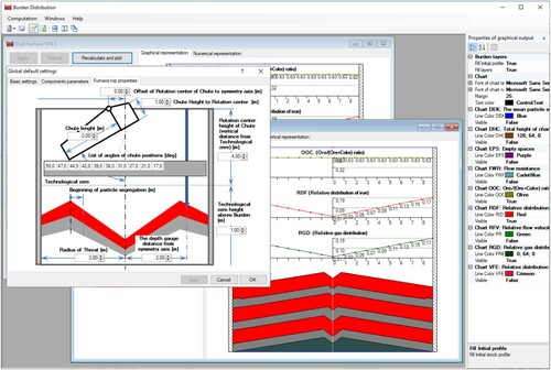
The dimensions and physical properties of the bell-less top charging system, charge properties, and other parameters of the simulation are set up in the global settings. We set these values only once at the beginning for a specific blast furnace or we edit them very rarely. The data in this program is set for all simulations in the Global Default Settings dialogue (see Figure 8). Here, the general parameters affecting the simulation calculation and its accuracy are also set. The program stores these settings in an XML configuration file, so it is possible to back up the configuration or create variations of the simulation calculation.

Figure 8. Global default settings dialogue.

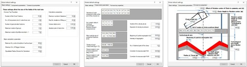
The second group of data is set individually for each simulation. There is no limit to the number of simultaneous simulations; the user only selects an item of New model simulation in the menu or clicks the icon and immediately a new window containing a simulation appears. This window has two parts (see Figure 9). In the left part, there is a panel with tabs, in which there are individual editing fields for inserting and editing simulation parameters. The input data for each simulation can be stored in a separate file from which they can be loaded. Therefore, the user can easily create different charging options just by modifying data and saving the file under a new name. All the values from the global settings are also stored in the file, so it is not dependent on the existing settings.

Figure 9. Graphic representation of burden layer profile with context menu for graphs choice.

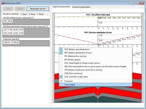
Upon pressing the button called Recalculate and plot, the result of the simulation presented in graphical or numerical form appears on the right side. After performing the calculation, we display the cross-section of the blast furnace throat with the profile of the individual charge layers on the right side of the window (see Figure 9). Above these layers, we can plot graphs with other calculated data as desired. The context menu with a menu of these graphs appears upon clicking the right mouse button above the graphical representation of the data. The user can then select any combination of graphs.

• RGD: Relative gas distribution

• RDF: Relative distribution of iron

• RFV: Relative flow velocity

• EPS: Empty spaces

• DHC: Total height of charge in each sector

• DEK: The mean particle size in a given sector over the entire column height

• VFE: Relative distribution of iron flow velocity

• FWR: Flow resistance

• OOC: Ore/(Ore + Coke) ratio.

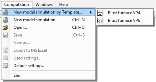
Of course, it is also possible to represent data graphically in various ways (colour of lines, font, etc.), which can be set in the Properties of the context menu. It is also possible to base calculations in the application on a template – these are XML files of the application with the prxt-extension stored in the application folder. This means that it is possible to add blast furnaces of different parameters or calculation variants by merely saving the pre-filled file. We can create a new entirely independent template by saving the performed simulation with the prxt-extension in the application folder. After this step, the template automatically appears in the computation menu (see Figure 10).

Figure 10. Menu of new model simulation by select the template.

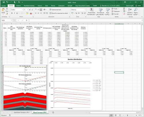
One unique feature is the ability to export all calculated simulation data into an MS Excel file. We must install MS Excel for this feature to work. The function is available from the menu offering Computation, or Export calculation to MS Excel menu. The menu activates after we have calculated the simulation. After selecting export, all computed data are exported into a new sheet and list with a name identical to the name of the simulation (it is possible to define the name when saving the simulation). The image of the simulation appears below the table data. Furthermore, the application automatically creates and implicitly places into a separate sheet a graph of the charge layer based on the calculated coordinates of the breaks in the layer profile. The output in MS Excel shows Figure 11.

Figure 11. Export MS Excel document.

Results and discussion

We can control the blast furnace in two standard ways, from the top and the bottom. Understanding and effectively managing the blast furnace operation is essential in reducing the cost per tonne of pig iron produced. Furthermore, it can be used as a preventive measure to avoid abnormal operating conditions, which are frequently caused by an incorrectly chosen distribution matrix. Historically, this problem has also occurred in the blast furnaces used at Třinecké železárny.

In November 2013, Třinecké železárny finished the investment project and started PCI (Pulverized Coal Injection) technology [15], which replaced approximately 1/3 of the previously used metallurgical coke in the charge with pulverized coal. This pulverized coal is injected directly into the blast furnace through the tuyeres. The implementation of PCI technology required a new distribution matrix. The correct choice of the loading matrix has a significant impact on the efficiency of the technology.

The managers and technologists of the Třinecké železárny blast furnace department were also aware of this. Already in 2013, the company ordered the development of a simulation system for modelling the blast furnace charge from the Technical University of Ostrava. In 2014, technologists began to use simulation software extensively to find the optimal method of loading the charge.

Before the implementation of Pulverized Coal Injection, 100% of the fuel was blast furnace coke, which not only serves as fuel in the blast furnace, but also ensures the permeability of the blast column, acts as a reducing agent, and a carburizing agent.

With the partial replacement of the coke charge by finely ground coal injected through tuyeres, there are, among other things, fundamental changes in the gas-dynamic conditions in the blast furnace. Because of these changes, it is necessary to adapt the loading matrices to ensure the permeability of the charge column and to avoid uneven running of the blast furnace or even the hanging of the charge and stopping the descent.

Using the Burden Distribution Application, the loading matrices were gradually optimized, and in addition to reducing the amount of coke by about 30%, the permeability of the central part of the charge column was increased by increasing the proportion of metallurgical coke (fraction above 40 mm).

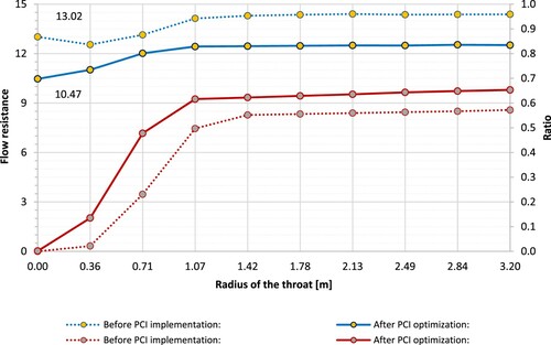
Figure 12 shows a comparison of the results of the loading matrices simulations before PCI injection (left) and after PCI optimization. The simulation results show that the resistance to flow in the central part of the charge is significantly reduced. A detailed comparison is illustrated by the graph in Figure 13, which shows a reduction of the average resistance to flow by 15% and even 25% in the centre of the furnace.

Figure 12. Result of burden distribution simulation before implementation PCI (left) and after PCI optimization (right).

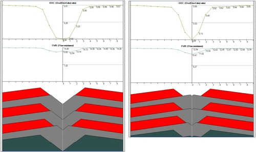
Figure 13. Comparison of significant burden distribution parameters before PCI implementation and after PCI optimization.

In some publications, simulation methods for layering the components of the charge in the blast furnace authors verified through scaled-down models of blast furnaces [7,8]. However, verifying and evaluating the benefits of the model under operational conditions is not easy. First, it is not possible to physically verify the actual state of the charge distribution. Second, it is not possible to guarantee that the parameters are invariant before and after the model is implemented.

In practice, the essential parameter indicating efficient production in a blast furnace is the specific fuel consumption (sum of metallurgical coke, minor coke fractions, and substitute fuels) per tonne of pig iron produced.

Significant is the efficiency of utilization of the reduction potential of the gas for indirect reduction of metal-bearing charge, which can be expressed by evaluating the composition of the blast furnace gas using the parameter $\eta \mathrm{C}\mathrm{O}$ (%) – carbon monoxide efficiency [16,17]. (37) $\eta \mathrm{C}\mathrm{O}={\displaystyle \frac{\mathrm{C}{\mathrm{O}}_2}{\mathrm{C}\mathrm{O}+\mathrm{C}{\mathrm{O}}_2}\cdot 100\text{\%}}$(37)

Thanks to the gradual optimization using the Burden Distribution Application, regular operation of the blast furnaces in the Třinecké Železárny Ironwork was achieved, and the achievement of a gas utilization rate of $\eta \mathrm{C}\mathrm{O}$ above 50% (for details, see Table 1).

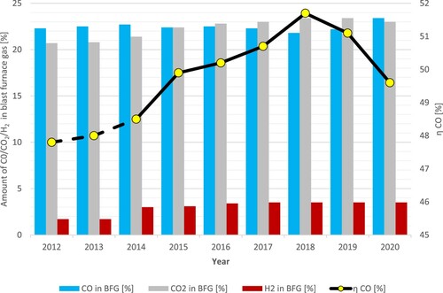
Table 1. Evolution of Blast Furnace Gas (GBF) composition and gas utilization eta CO.

Year	2012	2013	2014	2015	2016	2017	2018	2019	2020
CO in BFG [%]	22.3	22.5	22.7	22.4	22.5	22.3	21.8	22.2	23.4
CO2 in BFG [%]	20.7	20.8	21.4	22.4	22.8	23	23.4	23.4	23
H2 in BFG [%]	1.7	1.7	3	3.1	3.4	3.5	3.5	3.5	3.5
ηCO [%]	47.8	48	48.5	49.9	50.2	50.7	51.7	51.1	49.6

As the graph in Figure 14 illustrates, since the end of 2013, when PCI injection into the blast furnaces started, the optimization of the blast furnace loading has also succeeded in increasing the utilization of the reduction potential of the blast furnace gas ηCO from 48.5% to 51.7% with stable metal-bearing charge parameters. Values exceeding 50% indicate suitable control of the blast furnace process and serve to verify the blast furnace loading model. The decrease in 2020 is mainly due to production curtailment related to the COVID 19 pandemic.

Figure 14. Evolution of blast furnace gas composition and gas utilization ηCO.

Conclusions

The blast furnace charging simulation provides data, which are otherwise obtainable in very complicated and costly ways. The computational core of the simulation can utilize analytical calculation methods or other advanced finite element methods [18]. The main advantage of analytical methods is the significantly lower processing power requirement and thus the speed of the performed simulation. Such a solution is then considerably more accessible to blast furnace operators who can easily explore more variants of charging methods immediately.

We have chosen the analytical methods for calculating the layering of the material, including segregation and gas flow distribution based on the research of used charging simulation methods. We have programmed and implemented the procedures in the new charging program named Burden Distribution. We have described the calculations, including the proposed algorithms, in detail in the article. We have provided the data of the required input parameters of actively operated blast furnaces from the cooperation of the Research Center of Advanced Mechatronic Systems with a pig iron producer in the Czech Republic, the company Třinecké železárny.

The result is an application, which helps to find the optimal charging method and can quickly respond to consequences of changes of individual material properties or charging program parameters. The graphical representation of the simulation results gives a clear overview of the burden distribution, as well as the data about many of other observed quantities along the radius of the blast furnace stack. The application is user-friendly, although the entry of input data, given their nature, requires a highly qualified user who can define them correctly.

Another advantage is the ability to model various changes and defects of the bell-less top charging system quickly. If there is a defect in the positioning system of the chute, it is possible to find out what the consequences will be or it is possible to adjust the charging program for minimal negative effects. We have created the software on an order from the company Třinecké železáren for simulating the charging in blast furnaces.

Disclosure statement

No potential conflict of interest was reported by the author(s).

Additional information

Funding

This work was supported by the European Regional Development Fund in the Research Centre of Advanced Mechatronic Systems project, CZ.02.1.01/0.0/0.0/16_019/0000867 within the Operational Programme Research, Development and Education and the project SP2021/27 Advanced methods and technologies in the field of machine and process control supported by the Ministry of Education, Youth and Sports, Czech Republic.

References

- Radhakrishnan VR, Ram KM. Mathematical model for predictive control of the bell-less top charging system of a blast furnace. J Process Control. 2001;11:565–586.
- Saxén H, Hinnelä J. Model for fast evaluation of charging programs in the blast furnace. Miner Process Extr Metall Rev. 2004;25:1–27.
- Zhu Q, Lü C-L, Yin Y-X, et al. Burden distribution calculation of bell-less top of blast furnace based on multi-radar data. J Iron Steel Res Int. 2013;20:33–37.
- Nag S, Gupta A, Paul S, et al. Prediction of heap shape in blast furnace burden distribution. ISIJ Int. 2014;54:1517–1520.
- Matsuzaki S. Estimation of stack profile of burden at peripheral zone of blast furnace top. ISIJ Int. 2003;43:620–629.
- Kondoh M, Konishi Y, Okabe K, et al. Interprétation cinématique d essais de chargement à l échelle 1 dans un haut fourneau à gueulard sans cloche. Rev Met Paris. 1981;78:733–744.
- Mitra T, Saxén H. Model for fast evaluation of charging programs in the blast furnace. Metall Mater Trans B. 2014;45:2382–2394.
- Park J-I, Jung H-J, Jo M-K, et al. Mathematical modeling of the burden distribution in the blast furnace shaft. Met Mater Int. 2011;17:485–496.
- Mehta A, Barker GC. The dynamics of sand. Rep Prog Phys. 1994;57:383–416.
- Fu D, Chen Y, Zhou CQ. Mathematical modeling of blast furnace burden distribution with non-uniform descending speed. Appl Math Model. 2015;39:7554–7567.
- Rahman M, Shinohara K, Zhu HP, et al. Size segregation mechanism of binary particle mixture in forming a conical pile. Chem Eng Sci. 2011;66:6089–6098.
- Zhang J, Qiu J, Guo H, et al. Simulation of particle flow in a bell-less type charging system of a blast furnace using the discrete element method. Particuology. 2014;16:167–177.
- Yamada T, Sato M, Miyazaki N, et al. Distribution of burden materials and gas permeability in a large volume blast furnace. Kawasaki Steel Giho. 1974;6:16–37.
- Iwamoto N, Makino Y. State of sulphur in a synthetic blast furnace slag and relation between segregation of sulphur and morphology of primary phase. Tetsu-to-Hagane. 1983;69:220–227.
- Ishii K, Ariyama T, Japan HU. Advanced pulverized coal injection technology and blast furnace operation. Oxford: Pergamon; 2000.
- Azadi P, Minaabad SA, Bartusch H, et al. Nonlinear prediction model of blast furnace operation status. In: Sauro Pierucci, editor. Computer aided chemical engineering. Vol. 48. Milano: Elsevier; 2020. p. 217–222.
- Geerdes M, Chaigneau R, Lingiardi O. Modern blast furnace ironmaking: an introduction. 4th ed. Amsterdam: IOS Press; 2020.
- Zhou C, Tang G, Wang J, et al. Comprehensive numerical modeling of the blast furnace ironmaking process. JOM. 2016;68:1353–1362.