Acoustic emission monitoring to optimize the end-of-cast in blast furnaces

ABSTRACT

When tapping a blast furnace, a break-through of gas through the taphole at the end of a cast needs to be prevented, both to preserve a healthy state of the taphole and to prevent gas and dust from escaping into the environment. In this paper, two acoustic techniques are presented that can be used to prevent gas emissions from the taphole at the end of a cast. The first approach is by using the spectral analysis of the recorded data, the second approach uses a neural network to recognize the popping sounds that announce the slag–gas interface is approaching the taphole level. It was found that with both methods the end of the cast is detected about 4–2 min before the cast is ended.

KEYWORDS:

• Acoustics
• blast furnace
• machine learning
• tap hole

Introduction

For the safe operation of a blast furnace, sufficient iron and slag need to be drained to prevent flooding of the furnace. When the liquid level becomes too high in the furnace it will cause operational problems and potentially lead to dangerous situations [1]. On the other hand, tapping too much liquid from the furnace may result in short-circuiting of the hot blast and gas escaping via the taphole to the outside of the furnace. This causes damage to the taphole, releases gas and dust into the environment and causes severe spraying of the tap which is undesired [1]. Especially, the environmental issues caused by gas and dust release are important. One may estimate the levels of liquid iron and slag in the furnace to predict when the cast needs to be ended. An overview of different ways to estimate the liquid level in the blast furnace is given in [2]. A heat and mass balance computation seems a straightforward option, however such models need frequent fine-tuning to be used in practice. Thermocouple data and EMF sensors can be used to provide feedback to such models.

As the liquid-level models lack the required accuracy in practice, the end of cast is often judged by operators mainly by sight and hearing. At the end of the cast, the liquid may produce more and more sparks and may eventually start spraying. For the longevity of the taphole, it should be closed before severe spraying occurs. An audible indicator is the popping sound that is clearly heard at the end of the casting period. It is likely that the popping sounds are produced by gas bubbles released from the furnace.

In this work, audio recordings of the tap stream are analysed. Two different approaches were investigated to signal the end of the cast.

The first approach uses a broad frequency range extending beyond the audible range. From the detection of pipeline leakages, it is known that gas leaking through small holes produces high-pitched sounds. The leakage can be detected by locating the source of these high-pitched sounds. This way of detecting gas leakage is often used for detecting leakages in pipe systems conveying pressurized gas [3]. For this purpose commercial systems are available. No publications are known that use such methods or equipment for the detection of gas escape from a blast furnace.

The second approach is based on automated recognition of the sounds produced by the cast in particular the popping sounds at the end of a cast.

The liquids and gas bubbles may produce different sounds by various mechanisms and a good overview of these mechanisms is found in [4]. The liquid from the taphole drops down on the liquid in the trough thereby creating bubbles that collapse later. At the experiment locations, there is no sight on the location where the liquid emerging from the taphole comes down on the liquid in the trough due to the presence of the trough cover. Therefore, noise from the liquid falling onto the liquid in the trough is attenuated.

Another source is the gas bubbles that pop directly after leaving the taphole. The loud popping heard at the end of the cast is likely to come from the escaping gas bubbles. At the end of the cast the slag interface closes in on the taphole thereby making it possible for the gas to enter the taphole. One of the methods described in this paper focusses on the detection of these loud pops. A machine learning approach is used for the automated recognition of bursting events.

Machine learning techniques have emerged in many fields now including ironmaking. For example, the prediction of silicon content in the produced iron [5] or the prediction of the temperature of the hot metal [6].

With respect to recognition of the popping sounds in the nuclear industry, similar methods are being investigated for example to prevent a boiling crisis [7] by detecting the sound of the popping bubbles. Although efforts have been done to use acoustic analysis for the diagnosis of a blast furnace process [8], no publications were found that describe the analysis of the acoustic emission of the tap.

Problem analysis

To obtain hot metal from a blast furnace a hole is drilled into the wall of the hearth. The produced iron and slag will drain from the furnace until the point that the slag level will dip below the level at which the taphole is present. The gas pressure present above the slag is several bars above atmospheric pressure. When the slag level dips for a short period of time below the top of the taphole on the hot side a bubble will be trapped. These gas bubbles will travel up the taphole and escape from the furnace.

This process is illustrated in Figure 1. A vertical cross-section is shown through the middle of the taphole. On the left, the hot side of the furnace is depicted with at the bottom the liquid iron, on top of this a layer of liquid slag. In practice, this process is complicated by the unburned coke that piles up at the bottom of the furnace which is not illustrated here. The gray blocks illustrate the furnace refractory the thickness is about 1.5 m. The taphole is drilled under a slight angle and is a few centimetres in diameter. The taphole size will increase during the tap due to erosion. The brown cone illustrates the ‘mushroom’ that is formed due to the clay mass which is used to close the taphole at the end of each tap. Gas may also enter the tapholes through cracks in the refractory or mushroom.

Figure 1. Gas bubbles escaping via the taphole.

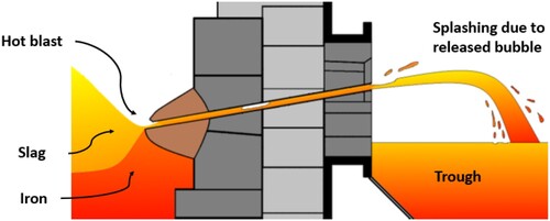
As the slag level drops further the bubbles will grow bigger and bigger. Due to the lower pressure on the outside of the furnace, the gas bubbles will expand and accelerate towards the outlet of the taphole and most likely are the cause of the splashing [9]. At the point that bubbles escape from the furnace, the taphole should be closed to prevent a gas break-through.

The goal of the reported research is to investigate if the acoustic measurements can assist in the decision to end the cast. The first step in this research is to be able to detect when gas is escaping from the furnace. The escaping gas needs to be detected in a timely manner such that a gas break-through is avoided, preferably no gas will escape from the furnace at all. Additionally, the resulting method for detecting the end of the cast can be used for the feedback to a liquid-level model for automatic recalibration.

Methods

Measurement setup

The measurements have been done using different types of microphones and two of them have a broad spectrum to include the ultrasonic range. The measurements were performed on both blast furnaces in IJmuiden.

The initial trials were performed with an AudioMoth device from Open Acoustic Devices [10]. The AudioMoth is a stand-alone recorder which supports a 384 kHz recording rate. The device was used to collect measurements for a period of 24 h. In this period 4 casts were recorded with a duration varying from 1 to 4 h. The device was set to record continuously and the recorded data were saved to a file. For each 10 min a file was saved to prevent losing the whole recording in case the device is not properly shutdown at the end of the experiment.

A later experiment was conducted using a Dodotronic UltraMic 384k [11] and a ReSpeaker 4-Mic array [12]. The latter is a small array microphone consisting of four microphones in a square arrangement. The microphones were connected to a Raspberry Pi 4 which was programmed to record the raw data from the microphones to an SD card. The maximum recording speed for the four channels simultaneously is 44 kHz. In 24 h, five casts were observed all with duration of about 2 h.

The microphones were placed at approximately 10 m from the tap to prevent damage from the heat radiation emitted from the tap.

In Figure 2, an example is shown of the amplitude of the signal versus time during a cast. The data were low-pass filtered to remove most of the hissing noise in the background.

Figure 2. Time signal of a recording, start and end are clearly marked by drilling and hissing.

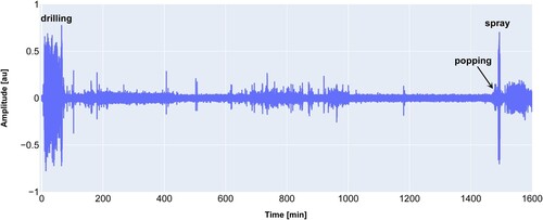
The start of a cast is clearly marked by the drilling of the taphole. At this particular furnace, a spray screen is activated at the closing of the taphole to prevent dust from escaping. This spray screen produces a loud hiss which clearly marks the end of cast.

During the cast, several noises are audible such as intercom speech.

In Figure 3, the time data of two pops are shown such that we can have an idea about the duration of the pop sounds. The power spectrum of each detected pop can be examined.

Figure 3. Time signal for two clearly audible pops and their corresponding spectrum.

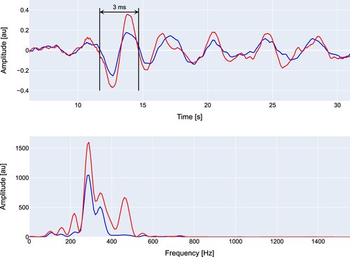
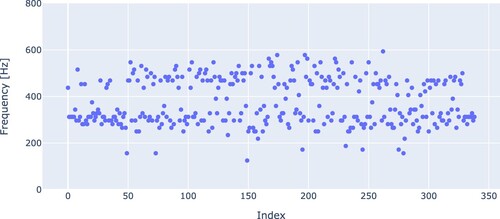
The frequency of the highest amplitude in the spectrum is then examined. In Figure 4, the result is shown over the course of a single cast. Two stranded bands are visible, which indicates the harmonics of the pop sound may often be more clear than the base frequency. This indicates that most of the energy of the popping sounds is found below 1 kHz.

Figure 4. Frequency of highest peak in the spectrum of the pop.

Spectral approach

In the spectral approach, the power spectra of the recordings are analysed. The steps of this analysis are schematically shown in Figure 5.

Figure 5. Steps in calculating the output of the spectral approach.

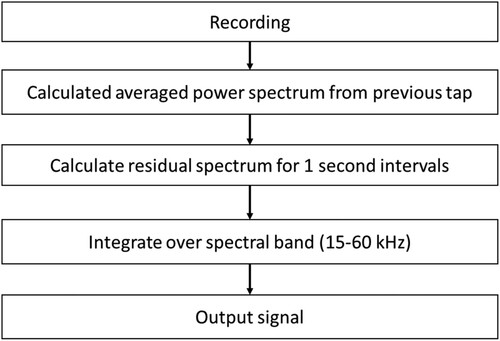
The first step in the analysis is to calculate an average spectrum over the cast period to capture the spectrum produced by background noise. There is a high amount of background noise present. As the spectral content of the noise is fairly constant the ensemble average of the spectra of the previous tap can be subtracted from the samples in the current tap.

The next step is to divide the recording into samples of 1 s duration. In each sample, an average power spectrum is calculated with a resolution of 1 kHz.

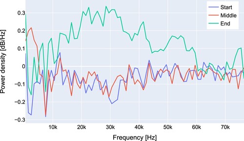
In Figure 6, the residual spectra are plotted for a sample in the first 10 min after the drilling of the tap hole, for a sample in the middle of the tapping cycle and for a sample just before the end of the tap. There is a clear bump visible in the spectrum from about 15–60 kHz.

Figure 6. Residual spectrum at the start, in the middle and at the end of a cast.

In the last step of the analysis, the spectral amplitudes are summed over the frequency band from 15 to 60 kHz.

Machine learning approach

At the end of a tap popping sounds of the bursting bubbles are clearly heard. Although humans can distinguish the pops easily by hearing it is quite hard to capture these sounds using analytical functions. In this case, machine learning techniques are valuable as they are very good in pattern recognition [13]. As machine learning is a very active field many new and different approaches emerge. A good overview of different approaches can be found in [14]. In this paper, the use of a simple neural network is explored.

In Figure 7, a simple neural network structure is depicted. The neural net consists of different layers. The first layer is the input layer where the input data are fed to the network. Each input neuron is connected to a neuron in the hidden layer. The input is weighted by a weighing factor w_i,j, where i is the number of the input neuron and j is the number of the neuron to which the neuron is connected. The neurons in the hidden layer may be connected to neurons in a deeper hidden layer. In this case, the neurons are connected to the output layer.

Figure 7. Simple neural network.

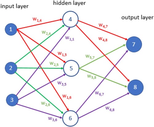
In our approach, the network is trained using labelled data, this approach is called reinforcement learning. During the training, the weights are updated using a training algorithm.

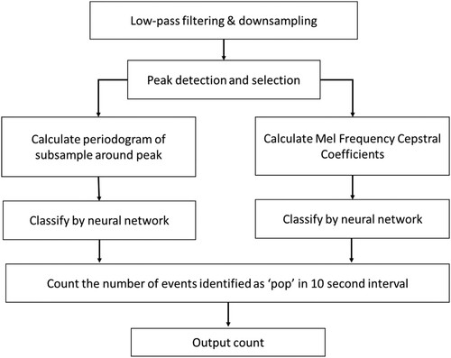
The popping sounds to be recognized produce short peaks which rise above the noise floor. To exploit this property a threshold algorithm is used. This algorithm calculates the standard deviation, σ, in the time window being analysed. Only peaks that have an amplitude higher than 4σ are selected for further analysis. The signal around the peak is sampled and processed before it is fed to the input of the neural network.

Two approaches are explored for producing the input to the network. The first approach simply calculates an average power spectrum of the input sample.

The second approach is a popular technique often encountered in speech recognition which is the use of Mel-Frequency Cepstral Coefficients (MFCC) [14]. This approach is popular as it tries to mimic the response of the human auditory system. The computation requires several steps being the computation of the power spectrum, mapping of the spectrum onto the Mel scale, taking the log of the resulting spectrum and finally a discrete cosine transform. In Figure 8, the steps of the algorithm are schematically depicted.

Figure 8. Steps in calculating the output for the neural net approach.

Results

Results spectral approach

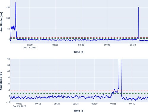
In Figure 9, the results are shown for the same cast shown in Figure 2. At the start and at the end of a cast large excursions are found due to the drilling and spraying noise at the end of the cast. If we zoom in on the end of the cast we see a rise in the signal. The standard deviation, σ, of the signal is calculated and the green dashed line is plotted at a level of 3σ and a red line indicates the 6σ level. The 3σ level is crossed at 1:52 min before the operator has decided to end the cast. This is crossed about 52 s before the end of the tap.

Figure 9. Results of the spectral approach for a cast. Top: complete cast. Bottom: Zoomed in to last minutes. The green dashed line indicates the 3σ level.

Results machine learning approach

For the recognition of pops, sounds no ultrasound range is needed and the recordings from the ReSpeaker array can be used in this approach.

The audio is processed in windows of 10 s. In this window, the standard deviation is calculated and only peaks that rise above a threshold of four times the standard deviation are selected for further analysis. Around the position of each peak, a small sample is taken of 150 ms (1200 samples), starting 50 ms before the peak.

In the next step, each peak is classified by a neural network. The amount of positively identified peaks in each window is counted.

The neural network needs to be trained using important features of the sample. From each sample, a short-term Fourier transform (STFT) is calculated using a sliding Hann window. The length is chosen to be 512 points and the hop length is set to 128 points, resulting in 10 spectra per sample. An average is calculated for these spectra. Due to aliasing this results in 256 unique values. These values are used as the input to the neural network.

For the training of the network, the position of the selected peaks throughout the recording is marked by human inspection with the default label being background noise. For the labelling, a free software tool called Audacity was used [15].

At the positions where a pop sound is audible the label is changed to ‘pop’. As a basis, a similar network is used for the classification of urban sounds [16].

The neural network was setup using Python using the Keras and SciPy packages. In the case where the averaged spectrum is used at the input the network consists of two densely connected layers with 256 neurons and one output layer with two neurons, corresponding to the two possible outcomes being ‘background’ or ‘pop’.

The first two layers have a rectified linear input activation and the last layer has a softmax activation. The softmax layer makes the output sum to one, such that the output of the two output neurons can be interpreted as a probability. When the probability of the output neuron representing the pop sound is above 50% the pop is counted.

Training of the network is performed using the Adam optimizer which uses a stochastic steepest-gradient approach for optimizing the weights in the network. A categorical cross-entropy is calculated for the loss function.

In Figure 10, the output of a training session is depicted, the network was trained on a single annotated cast. The set of background noises is much larger than the set of annotated pops. The pop count for this particular case is 170 pops versus 4433 background noises. The list of pops is equalized in size by random selection from the 170 pops. This brings the pre-training accuracy close to 50%, so no better than a random guess. The pop sounds are well discernable by the network and the accuracy quickly goes up to a high percentage. After 20 training epochs, the loss function flattens and 98% of the pops in the test set are correctly identified.

Figure 10. Example of training session of the neural network.

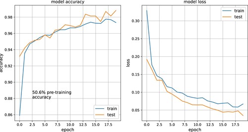
The training and test set are randomly generated and the test size consists of 20% of the samples from the complete data set.

Testing with different seeds for the random selection process all show similar behaviour.

The output layer of the network has two neurons representing the prediction of the network being a pop sound or not. If the probability of the neuron representing the pop output is above 50% the output is reported as a pop.

To determine whether the popping sounds are present during the cast the probabilities for each pop in each 10 s interval is summed. So only when all pops are identified with 100% certainty the amount of pops is equal to the output of the network. The lower bound of the output is thus half of the counted pops.

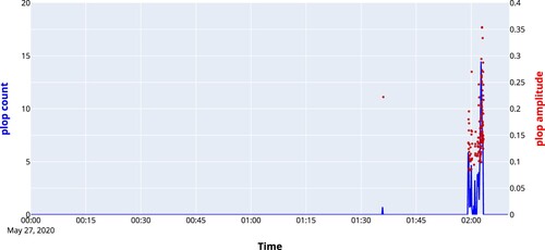
In Figure 11, the output signal is plotted for the end of a cast. In the same figure, the maximum amplitude of each sample is plotted in by a red dot. In the zoomed plot, it is found that there is quite a spread in the amplitudes of the detected pops, there is a gradual rise and an increasing spread visible.

Throughout the tap, there are pops detected which are mostly false positives. Only at the end of the tap, the signal shows a steep rise 2 min before the end of the tap.

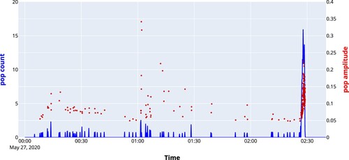
The UltraMic and ReSpeaker microphones were deployed simultaneously. Figures 11 and 12 show data from the same tap, however, the results presented in Figure 11 were recorded by the UltraMic and the results presented in Figure 12 were recorded by the ReSpeaker microphone array. For the recording with the microphone array, the counts at the output are higher than for the UltraMic (in total 332 versus 193) and there are less false detections throughout the tap. In Figure 13, the output of the network for another tap is displayed. This shows that also on a recording for which the network was not trained the output looks good. In this case, the popping was detected 4 min before the end of the cast.

Figure 11. Top: Output of the neural network based using spectral coefficients as input. Bottom: end of the cast.

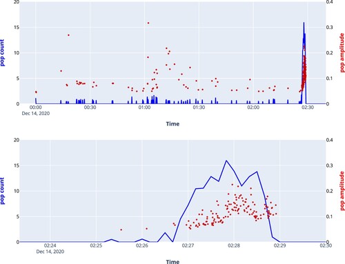
Figure 12. Output of the neural net using data from the ReSpeaker array.

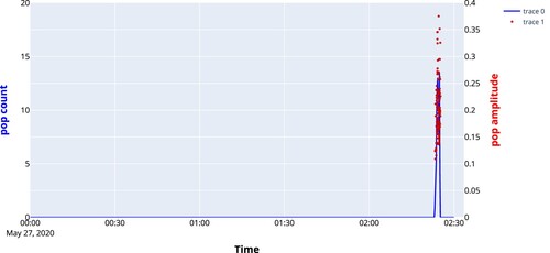
Figure 13. Output of the neural network for another cast using data recorded by the ReSpeaker 4mic array.

Reducing the Fast-Fourier Transform size of the (Short-time Fourier Transform) STFT from 256 to 128 points reduces the performance from 97% to 86% and the output becomes more noisy. When the amount of neurons in the first two layers is reduced from 256 to 128, still a similar performance is achieved compared to the STFT-based method. This reduces the amount of parameters of the model from 132,098 down to 22,018.

In Figure 14, the output is shown for a neural network where Mel-Frequency Coefficients are calculated to characterize each sample. In this case, only 40 inputs are used in the first layer instead of 256. Also, the hidden layer is downscaled to 40 neurons. The amount of trainable parameters goes down from 22018 to 3362 at the expense of more false positives.

Figure 14. Output of the neural network using MFC coefficient for the input.

Results spectral versus machine learning approach

In Figure 15, the output signal of both the spectral approach and the neural network is shown for the last 30 min of a tap. Both approaches show a steep rise just about 2 min before the tap hole is shut by the operator.

Figure 15. Spectral approach versus neural net.

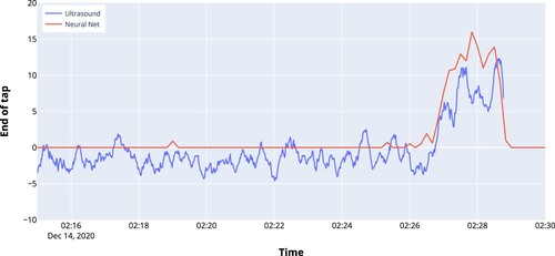
From recorded taps, the end of the cast was signalled from 90 to 240 s before the operator ended the cast. In the spectral method and the neural net approach, both signals start to rise at the same moment. However, the output of the spectral method is noisier which will make it more difficult to detect the end of the cast in a reliable way.

Discussion

The neural network has the advantage that a regular microphone may be used. In addition, a lower sample frequency is required. This also gives more flexibility for the enclosure of the microphone to shield it from the harsh environment at the blast furnace. The lower frequencies are less affected by protective screening, whereas for ultrasound this requires more careful engineering, the spectral results may benefit more from a directional microphone to block unwanted noise from the environment.

A convolutional network was trained in an attempt to improve the results. In this approach, the periodogram was not averaged over the data but all spectra are input to the convolutional network. No improvement was found. As the pops are pulse shaped there is also no necessity to shift a filter over the data as the best time slots to compute the spectra are already selected by the thresholding algorithm. In this way also computational power can be saved.

A hybrid method can be devised where the output of the spectral approach maybe used as an input for the neural network. The end of the cast is detected 4–2 min before the tap is ended. Earlier does not seem to be feasible due to the absence of the popping sounds. Possibly, when a microphone or accelerometer is mounted on the refractory close to the taphole the method can be improved. The spectral method can be improved by a directional microphone. However, closing the cast earlier may also not be desired as it is necessary to tap a sufficient amount of slag. With automated detection, it will be feasible to consistently close the tap which may already reduce the amount the gas escaping from the furnace and will improve safety and the environment.

Conclusion

A timely taphole closure can prevent dust and gas escape from the blast furnace. This is beneficial both for the environment and also for the condition of the taphole.

In this paper, two acoustic ways of detecting the end of a blast furnace tap are presented which detect the end of the tap 4–2 min before the taphole is closed.

One approach presented in this work takes advantage of the emission of sound in spectrum from 15 to 60 kHz. The other approach is recognition of the popping sounds produced by the bursting gas bubbles by a neural network. The output of both methods starts to increase at the same time. The spectral approach is more noisy and therefore less sensitive.

Disclosure statement

No potential conflict of interest was reported by the author(s).

Additional information

Funding

This work was carried out with a financial grant from the Research Fund for Coal and Steel within the Rihanne Project ‘Reliable Blast Furnace Hearth Management' [grant number 847332 (2019)].

References

- He Q, Zulli P, Tanzil F, et al. Flow characteristics of a blast furnace taphole stream and its effects on trough refractory wear. ISIJ Int. 2002;42:235–242.
- Agrawal A, Kothari AK, Ramna R, et al. A review on liquid level measurement techniques using mathematical models and field sensors in blast furnace. Metall Res Technol. 2019;116(3):307.
- Moon C, Brown WC, Mellen S, et al. Ultrasonic techniques for leak detection. In: SAE 2009 Noise and Vibration Conference and Exhibition; 2009.
- Langlois TR, Zheng C, James DL. Toward animating water with complex acoustic bubbles. ACM Trans Graph (TOG). 2016;35(4): 1–13.
- Zhou H, Zhang H, Yang C, et al. Deep learning based silicon content estimation in ironmaking process. IFAC-PapersOnLine. 2020;53(2):10737–10742.
- Jeménez J, Mochón J, Sainz de Ayala J, et al. Blast furnace hot metal temperature prediciton through neural networks-based models. ISIJ Int. 2004;44(3):573–580.
- Sinha KNR, Kumar V, Kumar N, et al. Deep learning the sound of boiling for advance prediction of boiling crisis. Cell Rep Phys Sci. 2021;2(3):1–14.
- Yenus J, Brooks G, Dunn M, et al. Application of vibration and sound signals in monitoring iron and steelmaking processes. Ironmak Steelmak. 2020;47(2):178–187.
- Qinglin HE, Zulli P, Tanzil F, et al. Flow characteristic of a blast furnace taphole stream and its effects on trough refractory wear. ISIJ Int. 2002;42(3):235–242.
- Hill AP, Prince P, Snaddon JL, et al. Audiomoth: a low-cost acoustic device for monitoring biodiversity and the environment. HardwareX. 2019;6:1–19.
- Dodotronic. Ultramic 384 K BLE, Dodotronic. [cited 2021 Aug]. Available from: https://www.dodotronic.com/product/ultramic-384k-ble/?v = 2a47ad90f2ae.
- ReSpeaker. ReSpeaker 4 Mic Array for Raspberry Pi. [cited 2021 Mar]. Available from: https://respeaker.io/4_mic_array/.
- Abu-Mostafa YS, Magdon-Ismail M, Lin H-T. Learning from data, vol. 4. New York: AMLBook New York; 2012.
- Khanafer M, Shirmohammadi S. Applied AI in instrumentation and measurement: the deep learning revolution. IEEE Instrum Meas Mag. 2020;23(6):10–17.
- McFee B, Raffel C, Liang D, et al. Librosa: audio and music signal analysis in Python. In: Proceedings of the 14th Python in Science Conference. Austin, TX; 2015, p. 18–24.
- Audacity. https://www.audacityteam.org, Audacity; 1999-2021.