A new multi-object tracking pipeline based on computer vision techniques for mussel farms

ABSTRACT

Mussel farming is a thriving industry in New Zealand and is crucial to local communities. Currently, farmers keep track of their mussel floats by taking regular boat trips to the farm. This is a labour-intensive assignment. Integrating computer vision techniques into aquafarms will significantly alleviate the pressure on mussel farmers. However, tracking a large number of identical targets under various image conditions raises a considerable challenge. This paper proposes a new computer vision-based pipeline to automatically detect and track mussel floats in images. The proposed pipeline consists of three steps, i.e. float detection, float description, and float matching. In the first step, a new detector based on several image processing operators is used to detect mussel floats of all sizes in the images. Then a new descriptor is employed to provide unique identity markers to mussel floats based on the relative positions of their neighbours. Finally, float matching across adjacent frames is done by image registration. Experimental results on the images taken in Marlborough Sounds New Zealand have shown that the proposed pipeline achieves an 82.9% MOTA – 18% higher than current deep learning-based approaches – without the need for training.

KEYWORDS:

• Object tracking
• computer vision
• object detection
• object description
• aquaculture
• mussel farming

1. Introduction

New Zealand is a world leader in premium seafood production. On a trajectory to becoming a $3 billion industry by 2035 (NZG 2019), New Zealand aquaculture is constantly evolving through research, innovation, and expansion. As production scales up, the demand for advanced software dedicated to aquafarm monitoring soars. Meeting this demand is where computer vision and artificial intelligence (AI) come into play. A new mode of aquafarming – technology-driven and highly scalable – is on the horizon. One of the pressing needs in New Zealand aquaculture right now is tracking mussel floats in mussel farms.

There are over 600 mussel farms in New Zealand. Currently, mussel farmers take regular boat trips out to the nearshore or open-ocean farm to check on mussel floats. It is a crucial yet labour-intensive assignment. As mussels grow in weight, more floats are required to keep the underwater crop lines both in place and at the most appropriate depth. Furthermore, mussel floats are vulnerable to rough seas – large waves can dislodge the floats and wash them away. Late replacements could potentially reduce crop yields. Therefore, there are great incentives to develop an automated system for tracking mussel floats. Such a system can also significantly reduce the number of boat trips required and help lower carbon footprints.

However, multi-object tracking in mussel farms is very challenging due to three main reasons.

(1)	First, the tracking targets in this real-world application are identical mussel floats in large quantities. Mussel floats are mass-produced products with similar appearances, making the identification of individuals difficult using conventional computer vision techniques. This problem is further compounded by the large number of targets within an image, which can be well over 50.
(2)	The second challenge is that the true image sampling rate in mussel farms is irregular due to data cleansing. Images are taken on a motorboat in the open ocean; thus, some are inevitably blurred. Getting rid of those subpar ones creates an unpredictable time gap between images, rendering trajectory prediction models ineffective. As a result, object tracking by imposing spatiotemporal constraints is not exploitable in this scenario, and we use object description rather than location for matching.
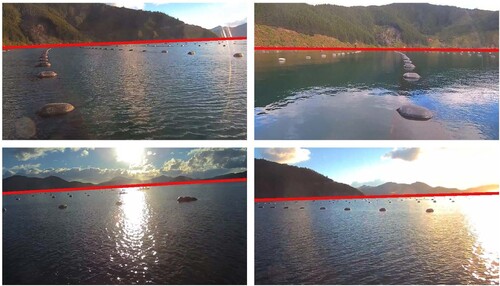
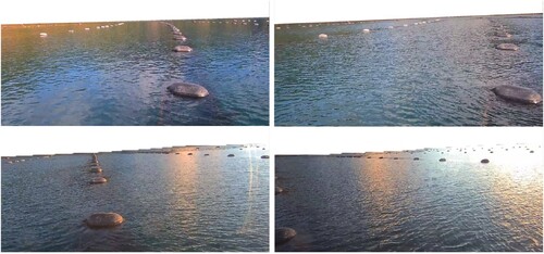
(3)	Finally, the image quality is often poor. Even the sharpest images after data cleansing are sometimes slightly out of focus, which requires a robust mechanism for object detection. Figure 1 shows four example images from the mussel farms at the Marlborough Sounds of New Zealand, each with a different viewpoint. The waterlines are marked in red. These examples demonstrate a great variety of image conditions due to wave conditions, weather, and daylight. In some cases, distant mussel floats are reduced to dots. Fortunately, although the camera is constantly moving, the floats are relatively stationary.

Figure 1. Example images from the mussel farms at the Marlborough Sounds of New Zealand.

Although numerous methods have been proposed for multi-object tracking (Bouraya Jr. and Belangour 2021; Ciaparrone et al. 2020; Yilmaz et al. 2006), their performance might be limited in this particular setting/task due to the above site-specific challenges. Our previous work has also attempted to detect floats or buoys from mussel farm images by using a genetic programming method (Bi et al. 2022). However, the method in Bi et al. (2022) only focused on object detection and it did not provide a solution to object tracking. To address the limitations of existing work and the above challenges, it is necessary to develop a new approach to multi-object tracking on mussel farm images.

The overall goal of this paper is to develop a new multi-object tracking pipeline for mussel farm images. The new approach comprises three main steps, i.e. float detection, float description, and float matching. It will be applied to a selection of mussel farm images acquired from Malborough Sounds, New Zealand. The performance of the proposed approach will be compared with two commonly used object-tracking methods based on deep neural networks.

The main contributions of this paper are summarised as follows

(1)	A new multi-object tracking approach with float detection, float description, and float matching is developed to automatically detect and track mussel floats in images.
(2)	A float detection method is developed to use various image processing operators, i.e. grey-world colour equalisation, homomorphic filtering, homography transformation, to process the input image and detect all floats of varying sizes in images.
(3)	A new float description method is developed to describe each mussel float using neighbouring floats' relative position.
(4)	A float matching method based on image registration is presented to find one-to-one correspondences across adjacent frames. This method is faster and more robust to sudden motion changes than point-matching methods.

This paper is organised as follows. Section ‘Background and related work’ provides the background of this paper and discusses related work on object detection and tracking. The proposed approach is introduced in Section ‘Proposed mussel float tracking approach’, followed by Section ‘Experiments and evaluations’, presenting the details of the experiments. The results are analysed and discussed in Section ‘Results and discussions’. Finally, Section ‘Conclusions’ concludes this paper.

2. Background and related work

This section describes the basic concepts of multi-object tracking and image registration. Then, it reviews the most related work on object detection and object tracking through image registration.

2.1. Background

2.1.1. Multi-object tracking

Multi-object tracking (MOT) is a task that locates multiple target objects in every frame of an image sequence while preserving their individual identities (Ciaparrone et al. 2020). MOT has attracted great interest in recent years due to the proliferation of high-performance cameras and computers. Although the pipeline for tracking varies according to the context in which they are conducted, MOT generally includes three key steps: object detection, object description, and object matching (Yilmaz et al. 2006). Figure 2 gives an example of an MOT task.

Figure 2. An example of a multi-object tracking task.

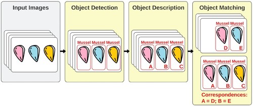
Typically, the input of an MOT system is a sequence of consecutive images, i.e. frames, and the output includes locations and unique identities of tracking targets in each frame. The first step is object detection, corresponding to determining the location of every object of interest in an image (Felzenszwalb et al. 2010). Non-target objects, if there are any, are discarded after this step. Locating the targets alone is not enough; they must be individually identifiable in order to make associations across frames. Object description does precisely that. It gives each target objects a unique marker based on its distinctive local features, which facilitates effective between-frame comparisons (Yang et al. 2011). Finally, object matching is the process of establishing one-to-one correspondences between targets in adjacent frames. This is done by using a loss function to formulate the association level between one detection in frame t and all objects in frame t + 1. The loss function is often defined by a combination of constraints such as proximity, relative velocity, and common motion (Veenman et al. 1998). For a target object, the detection with the lowest loss is its most plausible match in frame t + 1.

2.1.2. Image registration

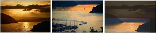
Image registration is an image alignment technique that combines multiple images into a single integrated scene (Zitova and Flusser 2003). This technique is predominantly applied to medical imaging and remote sensing. Figure 3, using two images by Vidar Nordli-Mathisen 2020, demonstrates an example of image registration. The first two images from the left capture the same scene from different angles. These two images can be spatially aligned by projecting one onto another's hyperplane, effectively overlapping the shared regions. The third image showcases this result. Objects that appear in both images will be aligned.

Figure 3. An example of image registration.

The planar projection of an image is achieved using a homography matrix. Mathematically, the transformation between two homogeneous 3D vectors p and q is expressed as (1) $q=Hp$(1) where H is a $3\times 3$ homography matrix with 8 degrees of freedom (Baer 2005). Four pairs of matching feature points are required to determine H. The most common detector-descriptor for image registration is SIFT (Lowe 1999), which uses image gradient magnitudes to describe and match feature points. Other alternatives include SURF (Bay et al. 2006), AKAZE (Alcantarilla and Solutions 2011), and BRISK (Leutenegger et al. 2011).

Image registration is a potential solution to multi-object tracking in mussel farms because the floats are immobile. While matching floats one by one is both time-consuming and prone to errors, image registration effectively overlays two images onto a common hyperplane and drastically reduces the chance of incorrect matches. Compared with conventional tracking approaches, where a high frame rate is critical to their performance, the image registration approach also takes a shorter time to execute due to a much lower frame rate requirement. Nonetheless, this tracking technique is built on the basis of a highly accurate image stitching process. If the fields of view overlap incorrectly, almost all matching attempts will fail.

2.2. Related work

2.2.1. Object detection

Object detection is the process of locating and classifying objects in images (Amit 2002). As the first step in multi-object tracking (MOT), object detection aims to find all tracking targets in every frame of an image sequence. In recent years, significant leaps in computational power have brought convolutional neural networks (CNN) to the spotlight. Liu et al. (2020) provided a thorough review of CNN-based object detectors.

Girshick et al. (2014) proposed regions with convolutional neural networks (RCNN) for object detection. Their ImageNet-based method searched for probable bounding boxes and extracted local features for detection (Krizhevsky et al. 2017). Then, objects were determined by a support vector machine (SVM) (Cortes and Vapnik 1995) classifier. Ren et al. (2015) proposed a faster version of RCNN, called Faster RCNN. Faster RCNN unified the search for probable bounding boxes, feature extraction, and classification into a single end-to-end learning framework, enabling close to real-time detection speed. You Only Look Once (YOLO) (Redmon et al. 2016) was one of the milestones in the progress of object detection. YOLO was extremely fast at over 100 frames per second. YOLO piled hundreds of predefined bounding boxes, called anchor boxes, across an image and calculated the probability of it containing an object. Probabilities and intersection over union (IoU) were used to fine-tune the anchor boxes for better results. Redmon and Farhadi (2017) and Redmon and Farhadi (2018) have made many improvements to YOLO to make it a popular and well-received deep learning-based object detector.

However, one of the main limitations of YOLO is its poor sensitivity to small object clusters (Redmon et al. 2016). This renders YOLO inappropriate for tracking mussel floats because most of the floats – apart from those close to the camera – look tiny in the images. Another limitation of applying YOLO to the mussel farm dataset is that YOLO works best with crisp images, but some of the mussel float images are blurry or out-of-focus. Although CNNs are generally more advanced in object localisation and classification power, they are not the best situational choice for this task. Traditional computer vision-based techniques for blob detection, such as the Laplacian filter (Haralick and Shapiro 1992) and the Laplacian of Gaussian filter (Horn et al. 1986), are a more suitable solution here because they are more straightforward, more robust against low image quality, and easier to deploy (no training required).

2.2.2. Object tracking through image registration

Mori et al. (2005) proposed a bronchoscope tracking method by combining magnetic sensor tracking and image registration. It was able to produce a tracking rate of one hertz during simulation. In a similar vein, Christensen et al. (2007) tracked the motion of human lung tissues during breathing using spirometry data and image registration. Their results on over 800 CT images showed that image registration was a practical tracking strategy with high accuracy. Fefilatyev et al. (2010) developed a marine vessel tracking algorithm based on image registration. Despite adverse tracking conditions such as unpredictable inter-frame position change, their algorithm achieved a significant increase in accuracy compared to the conventional methods. Their success proved that image registration was suitable for tracking objects with an unpredictable velocity.

Deep learning-based descriptors have emerged as a versatile solution to boost registration precision. Cheng et al. (2018) proposed a similarity network for image registration. The network was trained to learn the feature correspondence from well-defined registration instances based on a probabilistic loss function. De Vos et al. (2019) proposed an unsupervised deep learning approach to image registration in which no registration examples were required. It stacked multiple CNNs into a hierarchical architecture, achieving a coarse-to-fine registration process. Their method achieved a comparable registration accuracy to traditional techniques while being exponentially faster.

In scenarios where multiple objects within a scene stay in their positions, and only the viewpoint changes, image registration can be achieved through point set registration. One well-known method in this domain is Coherent Point Drift (CPD) (Myronenko and Song 2010). This method uses the object centres as feature points and bypasses the feature description step. The registration is done by maximising the likelihood of fitting one set of points onto the other. In this process, feature points serve as the centroids in Gaussian Mixture Models (GMMs). To improve image registration results, Locality Preserving Matching (LPM) (Ma et al. 2019) can be employed as an additional step after feature points matching. LPM reduces mismatches by maintaining the local neighbourhood structures.

The studies above have shown that object tracking through image registration is a fast and accurate strategy. However, these methods were not designed to track a large number of targets with confusing appearances, making them inapplicable for tracking mussel floats. Therefore, this paper proposes a new multi-object tracking approach for mussel farms to address these challenges.

3. Proposed mussel float tracking approach

The section describes the proposed approach to mussel float tracking, including three main steps, i.e. float detection, float description and float matching. Figure 4 illustrates the overall process with example images. The details of the three steps are as follows.

Figure 4. Flowchart of the proposed approach to mussel float tracking.

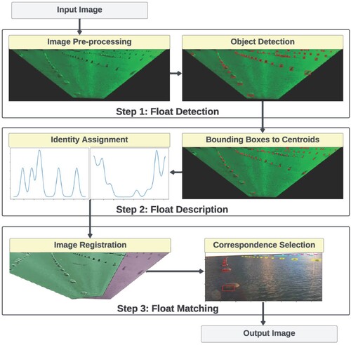
(1)	In the first step, input images undergo a series of pre-processing procedures designed to enlarge and better define the distant floats. Note that the images are first pre-processed to remove non-water regions using a waterline detection method in our previous work (McLeay et al. 2021). This waterline detection process significantly enhances detection power. Other techniques used in pre-processing include colour equalisation (Buchsbaum 1980), homomorphic filtering (Oppenheim et al. 1968), and planar projective transformation, i.e. homography. After pre-processing, a set of Laplacian of Gaussian filters (Horn et al. 1986) are employed to detect all the mussel floats in an image.
(2)	The second step is float description. A new feature descriptor is developed to assign a unique identity to each mussel float. The new descriptor is based on the relative positions of closeby neighbours, thereby independent of appearance. Bounding boxes are replaced by their respective centroid so that the relative positions of neighbours become more accurate.
(3)	Finally, one-to-one correspondences between detections in adjacent frames are established through image registration. This approach is faster and more robust to sudden motion changes than other point-matching methods. During image registration, homography transformation is made using the best pairs of matching floats and RANSAC (Fischler and Bolles 1981). Matches are then determined by a proximity measure.

3.1. Float detection

To detect floats from the images, a number of image pre-processing operations are employed. The pre-processing procedures are briefly described as follows.

• Grey-world colour equalisation. Images of the sea are predominately blue. Although colour does not directly affect the detection process, colour imbalance reduces overall contrast. The grey-world colour equalisation is thereby employed to deal with the colour imbalance. According to the grey-world assumption (Buchsbaum 1980), the average colour across all colour channels should be grey. Typically, each channel is individually adjusted to attain an average pixel intensity of 0.5 (out of 1.0), thereby fulfilling this assumption. Suppose C stands for any one of the colour channels (i.e. $C=\{R,G,B\}$), $C_{avg}$ is the average intensity across the entire image, $C(x,y)$ is the original pixel intensity at position $(x,y)$, and $C^{\mathrm{\prime }}(x,y)$ is the adjusted pixel intensity after grey-world colour equalisation. Then $C^{\mathrm{\prime }}(x,y)$ is given by: (2) $C^{\mathrm{\prime }}(x,y)=C(x,y)\times \frac{0.5}{C_{avg}}$(2)

• RGB to grey-scale. Due to the deficiency of red light in mussel farm images, the red colour is likely over-compensated after the grey-world colour equalisation. As a result, the colour image is converted to grey-scale to reduce the effect of over-saturation. The following conversion formula (Poynton 1998) works well for the data at hand because it is least sensitive to blue. Let $R(x,y)$ represent the red channel intensity at position $(x,y)$ etc., the resulting grey-scale intensity is calculated using: (3) $\mathrm{Grey}(x,y)=0.2126\times R(x,y)+0.7152\times G(x,y)+0.0722\times B(x,y)$(3)

• Homomorphic filtering. Illumination imbalance is a real problem in object detection because the detector's power deteriorates in darker regions. Homomorphic filtering is a brightness re-balancing procedure that maps a spatial image into the frequency domain, applies filters, and then maps it back to the original domain (Oppenheim and Schafer 2004). This process works best in reducing multiplicative noise. In this application, we apply a Butterworth highpass filter (Adelmann 1998) in the frequency domain to attenuate the low frequencies. Consequently, regions with similar intensities in the input image become zero after the highpass filter. Regions with a high intensity gradient, represented by the high frequencies, remain unaffected. When applied to grey-scale images, it simultaneously removes non-uniform brightness and enhances contrast for the less illuminated regions.

• Homography transformation. In this transformation, perspectives are altered to make the distant floats larger, sparser, and more apparent, thereby reducing the number of false negatives. The homography transformation is done by applying a $3\times 3$ homography matrix to every pixel location. As the viewpoint changes, distant floats will become more visible. However, the amount of information embedded in an image was fixed the moment it was taken. Therefore, there is no incentive to scrutinise the homography parameters. We aim for a good enough and generalisable homography that does not require case-by-case calibration. Therefore, preliminary tests have led to the identification of the homography illustrated in Figure 5, which works well across a wide range of mussel farm images. The corresponding homography matrix is given in Equation (4(4) $H=\left[\begin{array}{ccc}-5.427\times {10}^{-1}& -3.291& 8.886\times {10}^3\\ 0& -2.609& 4.993\times {10}^3\\ 0& -5.714\times {10}^{-4}& 1\end{array}\right]$(4) ). (4) $H=\left[\begin{array}{ccc}-5.427\times {10}^{-1}& -3.291& 8.886\times {10}^3\\ 0& -2.609& 4.993\times {10}^3\\ 0& -5.714\times {10}^{-4}& 1\end{array}\right]$(4)

Figure 5. An illustration of the employed homography. The four corners of the original image are shown in black, while the corners after transformation are shown in red.

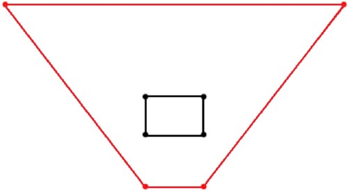
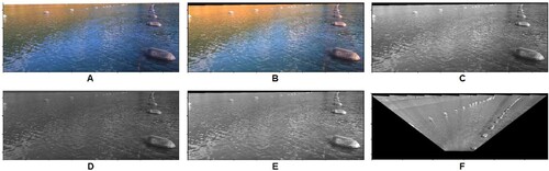
Figure 6 gives a demonstration of the preprocessing procedures. After homography transformation, a number of Laplacian of Gaussian (LoG) filters (Horn et al. 1986) are used for mussel float detection. LoG filters with different kernels can detect objects of various sizes. On the mussel farm images, the kernel size from $14\times 14$ to $18\times 18$ are chosen based on image resolution and aspect ratio.

Figure 6. A demonstration of the preprocessing procedures. A, input image; B, the first grey-world colour equalisation; C, RGB to grey-scale; D, homomorphic filtering; E, the second grey-world colour equalisation; F, homography transformation.

3.2. Float description

A new float description method is developed as a component of the proposed pipeline to assign unique identities to mussel floats. This is a difficult task because the mussel floats are confusingly similar in appearance. Therefore, a new application-specific descriptor based on relative positions rather than local features is adopted. It is somewhat similar to identifying a star in the night sky. In stargazing, the relative positions of stars are crucial because stars all look the same. Stargazers often begin with a star's neighbouring constellations and go from there. For example, suppose we are to find Sirius at night, we first need to spot Orion's Belt. Then draw a line through the Belt with Rigel on the left and Betelgeuse on the right. Sirius is somewhere near the line extension.

The proposed descriptor works in a similar vein. The unique identity of a mussel float is provided by two sets of numbers – the true bearings and the relative bearings. A true bearing to a neighbour is the clockwise angle measured from the upward direction. In a sense, the set of true bearings gives a mussel float an identity defined by where its neighbours are. For example, let X denote the set of mussel floats in an image, $X=\{X_1,X_2,\dots ,X_n\}$, and let U represent the upward direction, then the set of true bearings TB for an arbitrary float $X_k$ is given by (5) $T{B}_k=\{\mathrm{\angle }U{X}_k{X}_i|1\le i\le n,i\ne k\}.$(5) However, some floats may share a similar arrangement of neighbours. Therefore we use relative bearings to refine the identity further. The relative bearings of a target mussel float are determined by aggregating the true bearings from all neighbouring floats, while excluding the true bearing towards the target itself. In addition, these angles are oriented relative to the target's position rather than being measured from the upward direction. For example, the set of relative bearings RB for the mussel float $X_k$ is (6) $R{B}_k=\{x-\mathrm{\angle }U{X}_j{X}_k|x\in T{B}_j\mathrm{\setminus }\{\mathrm{\angle }U{X}_j{X}_k\},1\le j\le n,j\ne k\}.$(6) All angles are clockwise angles. The two sets of bearings tell us, in an intuitive way, where its neighbours are and who the neighbours are.

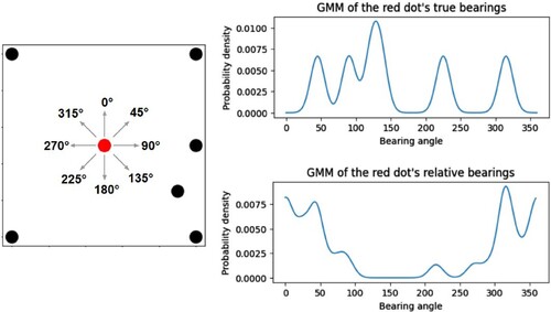
The bearing angles are dependent on viewpoints. Between two consecutive images, the bearing angles associated with the same mussel float are likely to change due to a shift in viewpoint. To compensate for discrepancies, each bearing angle is represented as a Gaussian distribution with mean μ and standard deviation σ, as opposed to a single number. A set of bearings is therefore represented by a Gaussian mixture model (GMM). This approach enables more accurate matching of mussel floats across different images even when the bearing angles are not exactly the same. Figure 7 provides an illustrative example. Considering the neighbouring dots, the set of true bearings for the red dot positioned at the centre of the image is $\{$45,90,122,135,225,315$\}$. The plot on the right shows the corresponding GMM with these means. The most pronounced peak on the plot (observed within the 100 to 150 range) comes from the merging of two separate peaks. These two peaks correspond to the black dots represented by the true bearings at 122 and 135 degrees respectively.

Figure 7. An illustrative example showcasing the Gaussian mixture models derived from the sets of true and relative bearings of the red dot.

3.3. Float matching

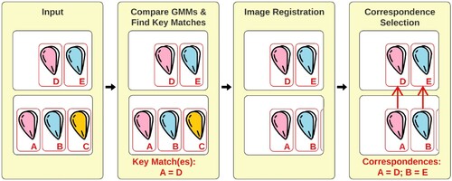
This is the last step in the proposed multi-object tracking pipeline. By this stage, every mussel float detection should have two GMMs as its unique identity. Float matching starts with comparing the GMMs, as shown in Figure 8. Next, the best matches are selected as keys for image registration. Finally, correspondences between two images are established by selecting the closest match that appears at a similar location after alignment.

Figure 8. Flowchart of the proposed approach to mussel float matching.

We employ a likelihood function to measure the degree of association between two mussel float detections. The objective is to identify the parameters, i.e. the means of a GMM, that optimise the likelihood of fitting the GMM to a given set of angles. If we have the true bearings of the target denoted as $x_1,x_2,\dots ,x_n$, and a candidate's true bearings represented by the means of a GMM as ${\mu }_1,{\mu }_2,\dots ,{\mu }_m$, with a common standard deviation σ, suppose f represent the Gaussian function, the likelihood L of fitting this GMM to the given data can be expressed as (7) $L=\prod _i\sum _{j}f(x_i|{\mu }_j,\sigma )$(7) where $i=1,2,\dots ,n$ and $j=1,2,\dots ,m$.

In order to attain rotation-invariance, the true bearings of the target can be uniformly adjusted by adding the same arbitrary angle to each element. This ensures that the likelihood remains independent of rotational transformations. For a given target in frame t, the most probable match for it in frame t + 1 is the one with the highest likelihood L. If there are multiple potential matches with similar levels of likelihood, comparing their relative bearings in a similar manner will reveal a winner. After matching the first few pairs to allow for image registration, float matching will be based solely on proximity. This strategy saves a considerable amount of computation resources because likelihood evaluation is time-consuming. Furthermore, this pipeline uses temporal information across frames to increase detection precision and accuracy. For example, a detection that only occurs in one frame but not the next has a high chance of being a false positive.

4. Experiments and evaluations

This section presents the dataset used in the experiments and the comparison methods. It also introduces the performance metrics used in the comparison.

4.1. Dataset

The proposed multi-object tracking pipeline's performance is evaluated on real mussel farm images from the Marlborough Sounds of New Zealand. The dataset includes 44 images sized $1080\times 1920$, extracted from four different videos. These four videos were taken at different times of the day and on different dates. Each image captures $20\sim 60$ partially submerged mussel floats. The new pipeline will begin with pre-processed images, i.e. images with the non-water region identified and removed. Figure 9 shows four examples. These images demonstrate a wide range of image conditions, including variations in picture quality, colour contrast, illumination, and viewpoint. In some cases, sea waves are so problematic that the mussel floats become hard to see. In addition, these images are sampled at irregular time intervals and from varying viewpoints.

Figure 9. Example mussel farm images with the non-water region removed.

The goal of the experiments is to evaluate both the object detection performance and the object tracking performance of the proposed pipeline. The following steps are performed on each image to obtain the detection and tracking results.

(1)	Employ image processing techniques to enlarge and better define the mussel floats barely visible in the far background;
(2)	Employ the new object detector made up of various traditional image processing operators to locate mussel floats;
(3)	Employ the new object descriptor and use the best matched features as keys to perform image registration;
(4)	Match mussel floats across adjacent frames based on a proximity measure;
(5)	Evaluate the detection and tracking performance.

4.2. Comparison methods

To demonstrate the effectiveness of the proposed pipeline, we employ two representative comparison methods: YOLO + SIFT + LPM and YOLO + CPD + LPM. Details of the two methods are summarised in Table 1. YOLO, SIFT are chosen because they are widely used methods for object detection and object description, respectively. CPD presents an alternative approach for image registration, circumventing the need for individual object description. LPM is an add-on process to reduce mismatches and enhance the quality of image registration.

Table 1. The proposed pipeline and comparison methods.

Method Name	Object Detection	Object Description	Object Matching
Proposed pipeline	New detector	New descriptor	Image registration using new descriptor
YOLO + SIFT + LPM	YOLOv8	SIFT	Image registration using SIFT + LPM
YOLO + CPD + LPM	YOLOv8	N/A	Image registration using CPD + LPM

In the two comparison methods, the YOLO model is the pretained eighth version with the creator's recommended configurations (Jocher et al. 2023). The confidence score is set to $25\text{\%}$. In addition, YOLOv8 is further fine-tuned on annotated mussel farm images. Online data augmentation is used during the training process. SIFT and CPD are tried-and-true methods. They either use the default configuration in the Python's OpenCV package or an empirically tuned configuration.

4.3. Performance evaluation

The most widely used performance metric for multi-object tracking is the multiple object tracking accuracy (MOTA). MOTA is an expressive metric with components covering both object detection and multi-object tracking. Let $F{N}_t$ be the number of false negatives in frame t; $F{P}_t$ be the number of false positives in frame t; $IDS{W}_t$ be the number of identity switches or mismatches during tracking in frame t; and $G{T}_t$ be the number of ground truth instances in frame t; MOTA is expressed as (8) $\mathrm{MOTA}=1-\frac{\sum _t(F{N}_t+F{P}_t+IDS{W}_t)}{\sum _{t}G{T}_t}.$(8) Besides MOTA, three performance metrics are used to evaluate the detection power, i.e. Precision, Recall, and F1 score. The respective formulae are given below. (9) $\mathrm{Precision}=\frac{TP}{TP+FP}$(9) (10) $\mathrm{Recall}=\frac{TP}{TP+FN}$(10) (11) $\mathrm{F}1\mathrm{score}=\frac{2\times \mathrm{Precision}\times \mathrm{Recall}}{\mathrm{Precision}+\mathrm{Recall}}$(11) where TP is the sum of true positive detections, FP is the sum of false positive detections, and FN is the sum of false negative detections.

Bounding box detections are classified according to the following criteria. A bounding box touching a true mussel float is considered a true positive. Conversely, a false positive occurs when a bounding box contains no trace of a mussel float. If multiple bounding boxes are assigned to the same float, only one is considered a true positive, while the remaining ones are considered false positives. A false negative indicates a missed detection.

5. Results and discussions

This section compares the new approach and the comparison methods in terms of float detection performance and float tracking performance.

5.1. Float detection results

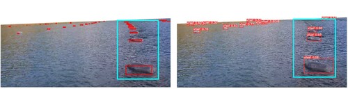
The object detection results of the same image by different methods are compared. Figure 10 shows the outcomes from the new detector (left) and YOLOv8 (right). Despite challenging detection conditions, including dense ocean ripples, low image quality, and low contrast, the new detector effectively distinguishes mussel floats from non-objects and ripples. In comparison, YOLOv8 struggles to detect mussel floats accurately due to low image quality. When the mussel floats cluster closely together, such as the ones inside the cyan box shown in Figure 10, YOLOv8 is only able to detect the first three instances closest to the camera. In contrast, our new detector successfully identifies nine.

Figure 10. Float detection results obtained by the new mussel float detector (left) and the YOLOv8 method (right) on the same image.

However, the bounding boxes produced by the new detector do not always include the whole object. Consequentially, centroids used for image registration are not precise geometric centres and may slightly weaken the tracking power. Therefore, the new detector obtains better mussel float detection performance than YOLOv8 at the cost of bounding box precision. Table 2 compares the detection results for the Marlborough dataset. The 1746 test instances come from 44 images extracted from 4 different videos, while the 425 training instances for YOLOv8 come from another 14 images extracted from the same videos.

Table 2. Comparison of object detection methods

Method	Training set	Testing set	Precision	Recall	F1 score
New detector	No training required	1746 instances	91.7%	98.5%	95.0%
YOLOv8	425 instances	1746 instances	93.4%	88.8%	91.1%

Both object detection methods demonstrate precision levels over 90%, indicating a low number of false positives. This is good news for the subsequent object description and matching steps as false positives can impair tracking efficiency. The new detector achieves a much higher recall rate of 98.5% compared to YOLOv8's 88.8%. This result supports the supposition that the new detector is a better situational solution due to its straightforward mechanism and robustness against low-quality images. The two methods have comparable F1 scores, with the new detector achieving 95.0% and YOLOv8 achieving 91.1%. Although YOLOv8 has a training stage, it does not translate into a higher F1 score.

For the new detector, the primary cause of false positives is multiple hits on the same object. Meanwhile, false positives resulting from dark patches of water are hard to eliminate since these patches are also alien objects on the ocean surface, making them indistinguishable from the actual targets. YOLOv8's built-in classification feature reduces some false positives but not by much. This is because only one class of object is of interest. False negatives are predominantly mussel floats buried deep in the far background. While there are ways to increase the new detector's recall further, this could also result in more false positives due to higher sensitivity to small objects. To sum up, the new detector is a better all-round solution for the mussel float detection task, despite having lower bounding box precision than YOLOv8.

5.2. Float matching and tracking results

Given that the effectiveness of the new descriptor is only discernible during the matching process, where incorrect matches indicate inconsistent labelling and thus an ineffective object descriptor, we conduct a joint evaluation of the description and matching performance.

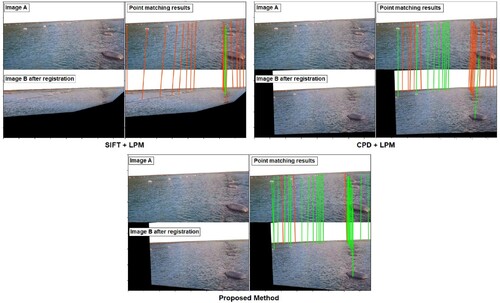
First we examine the matching results using the ground truth correspondences to obtain an objective evaluation. Figure 11 gives an example comparison of mussel float matching using SIFT + LPM, CPD + LPM, and the new descriptor. Incorrect matches are indicated by red lines, and correct matches are indicated by green lines. The SIFT + LPM results show that image registration is a feast-or-famine approach, where poor image registration will lead to mismatches for almost all objects. In this example, CPD + LPM outperforms SIFT + LPM by correctly matching the prominent mussel floats. However, CPD + LPM struggles to establish accurate correspondences for those located far away from the camera. Moreover, the effectiveness of CPD + LPM deteriorates when there are instances of objects entering and exiting between the two images. In comparison, the new descriptor achieves accurate alignment of the two images and successfully matches almost all mussel floats.

Figure 11. Float matching results using SIFT + LPM (top left), CPD + LPM (top right), and the proposed method (bottom) on the same image. Mismatches are indicated by red lines, and correct matches are indicated by green lines.

In terms of matching, the number of test instances is lower as there are fewer mussel floats present in the shared scene. Table 3 summarises the mismatch rates for all three methods using the ground truth correspondences. CPD + LPM has the highest mismatch rate of 20.5%. As a point correspondence method, CPD + LPM is less affected by image conditions but prone to mismatches when there is a high density of mussel floats in an image or a significant number of object entries and exits. SIFT + LPM follows closely with a mismatch rate of 18.9%. Since it relies on appearance-based features, SIFT + LPM tends to fail disastrously under challenging image conditions such as low resolution and poor lighting. In contrast, the new descriptor outperforms the other methods with the lowest mismatch rate of 8.9% among the three. As a point correspondence method, the new descriptor demonstrates greater robustness when dealing with a larger number of points compared to CPD + LPM.

Table 3. Comparison of object description and matching methods using the ground truth correspondences.

Method	Testing set	Mismatch rate
New descriptor	1327 instances	8.9%
SIFT + LPM	1327 instances	18.9%
CPD + LPM	1327 instances	20.5%

Finally we examine the overall tracking performances of the three pipelines from detection to matching. Table 4 summarises the results for the Marlborough dataset. Keep in mind that MOTA also reflects false negatives and false positives carried over from the detection step. The proposed pipeline achieves the highest 82.9% MOTA, followed by YOLO + SIFT + LPM at 64.2%. YOLO + CPD + LPM is the worst among the three methods at 58.2%. Like many other deep learning-based detectors, the powerful classification ability of YOLO is underutilised in this application because there is only one class of objects in the images. Although YOLO produces accurate bounding boxes, it struggles when it comes to tracking a swarm of tiny objects. With MOTA below 85% across the board, none of them can be considered excellent for the multi-object tracking task. Mismatches play a significant role in the low MOTA observed. In cases where image registration is inaccurate, many correct mussel float detections end up as mismatches.

Table 4. Comparison of the overall tracking performances.

Method	MOTA
Proposed pipeline	82.9%
YOLO + SIFT + LPM	64.2%
YOLO + CPD + LPM	58.2%

5.3. Limitations

The new descriptor, while effective, has the limitation of requiring at least two mussel float lines in each image. If all the neighbours belong to the same line, the new descriptor will not function as intended. Another limitation of the proposed pipeline is that the new detector produces imprecise bounding boxes, leading to imperfect image registration outcomes. Despite these imperfections, the proposed approach remains the most successful among the three methods for tracking mussel floats in real-world images.

6. Conclusions

Traditional computer vision techniques are highly effective in various real-world applications. In this paper, we describe one such application: multi-object tracking for mussel farms. Compared to deep learning-based methods, this paper shows that traditional computer vision techniques offer several advantages in this specific domain: they are easily implementable and can be effective without requiring a substantial amount of training data, and they are in general less resource-intensive.

The proposed pipeline was assessed using a dataset of mussel farm images and showcased its proficiency in simultaneously tracking multiple identical targets. In the experiments, the new detector outperformed a state-of-the-art deep learning-based detector, and contributed to better overall tracking results. More importantly, the proposed pipeline was more robust than the comparison methods against low image quality and varying outdoor conditions, further enhancing its suitability for real-world applications. While this paper presents promising results for the mussel float tracking task, there is still a lot of room for improvements. Our future research will focus on improving runtime and reducing mismatches.

Acknowledgments

We would like to thank Max Scheel at Cawthron Research Institute for providing datasets, and Chris Cornelisen for his guidance as the Leader of SfTI Spearhead Project on Precision Farming.

Disclosure statement

No potential conflict of interest was reported by the author(s).

Additional information

Funding

This work was supported in part by the Science for Technological Innovation Challenge (SfTI) fund under contract 2019-S7-CRS and MBIE Data Science SSIF Fund under the contract RTVU1914.

References

- Adelmann HG. 1998. Butterworth equations for homomorphic filtering of images. Comput Biol Med. 28(2):169–181. doi: 10.1016/S0010-4825(98)00004-3
- Alcantarilla PF, Solutions T. 2011. Fast explicit diffusion for accelerated features in nonlinear scale spaces. IEEE Trans Pattern Anal Mach Intell. 34(7):1281–1298. doi: 10.5244/C.27.13
- Amit Yali. 2002. 2D object detection and recognition: models, algorithms, and networks. MIT Press.
- Baer R. 2005. Linear algebra and projective geometry. Courier Corporation.
- Bay H, Tuytelaars T, Van Gool L. 2006. Surf: speeded up robust features. In European Conference on Computer Vision; Springer. p. 404–417.
- Bi Y, Xue B, Briscoe D, Vennell R, Zhang M. 2022. A new artificial intelligent approach to buoy detection for mussel farming. J R Soc N Z. 53(1):27–51. doi: 10.1080/03036758.2022.2090966
- Bouraya Jr. S, Belangour A. 2021. Multi object tracking: a survey. In: Thirteenth International Conference on Digital Image Processing (ICDIP 2021); Vol. 11878; SPIE. p. 142–152.
- Buchsbaum G. 1980. A spatial processor model for object colour perception. J Frankl Inst. 310(1):1–26. doi: 10.1016/0016-0032(80)90058-7
- Cheng X, Zhang L, Zheng Y. 2018. Deep similarity learning for multimodal medical images. Comput Methods Biomech Biomed Eng Imaging Visual. 6(3):248–252. doi: 10.1080/21681163.2015.1135299
- Christensen GE, Song JH, Lu W, El Naqa I, Low DA. 2007. Tracking lung tissue motion and expansion/compression with inverse consistent image registration and spirometry. Med Phys. 34(6Part1):2155–2163. doi: 10.1118/1.2731029
- Ciaparrone G, Luque Sánchez F, Tabik S, Troiano L, Tagliaferri R, Herrera F. 2020. Deep learning in video multi-object tracking: a survey. Neurocomputing. 381:61–88. doi: 10.1016/j.neucom.2019.11.023
- Cortes C, Vapnik V. 1995. Support-vector networks. Mach Learn. 20(3):273–297. doi: 10.1007/BF00994018
- De Vos BD, Berendsen FF, Viergever MA, Sokooti H, Staring M, Išgum I. 2019. A deep learning framework for unsupervised affine and deformable image registration. Med Image Anal. 52:128–143. doi: 10.1016/j.media.2018.11.010
- Fefilatyev S, Goldgof D, Lembke C. 2010. Tracking ships from fast moving camera through image registration. In: 2010 20th International Conference on Pattern Recognition; IEEE. p. 3500–3503.
- Felzenszwalb PF, Girshick RB, McAllester D, Ramanan D. 2010. Object detection with discriminatively trained part-based models. IEEE Trans Pattern Anal Mach Intell. 32(9):1627–1645. doi: 10.1109/TPAMI.2009.167
- Fischler MA, Bolles RC. 1981. Random sample consensus: a paradigm for model fitting with applications to image analysis and automated cartography. Commun ACM. 24(6):381–395. doi: 10.1145/358669.358692
- Girshick R, Donahue J, Darrell T, Malik J. 2014. Rich feature hierarchies for accurate object detection and semantic segmentation. In: Proceedings of the IEEE Conference on Computer Vision and Pattern Recognition; p. 580–587.
- Haralick R, Shapiro L. 1992. Computer and robot vision. Vol. 1. Addison-Wesley Publishing Company; p. 346.
- Horn B, Klaus B, Horn P. 1986. Robot vision. MIT Press.
- Jocher G, Chaurasia A, Qiu J. 2023 Jan. YOLO by ultralytics. https://github.com/ultralytics/ultralytics.
- Krizhevsky A, Sutskever I, Hinton GE. 2017. Imagenet classification with deep convolutional neural networks. Commun ACM. 60(6):84–90. doi: 10.1145/3065386
- Leutenegger S, Chli M, Siegwart RY. 2011. Brisk: Binary robust invariant scalable keypoints. In: 2011 International Conference on Computer Vision; IEEE. p. 2548–2555.
- Liu L, Ouyang W, Wang X, Fieguth P, Chen J, Liu X, Pietikäinen M. 2020. Deep learning for generic object detection: a survey. Int J Comput Vis. 128(2):261–318. doi: 10.1007/s11263-019-01247-4
- Lowe DG. 1999. Object recognition from local scale-invariant features. In: Proceedings of the Seventh IEEE International Conference on Computer Vision; Vol. 2; IEEE. p. 1150–1157.
- Ma J, Zhao J, Jiang J, Zhou H, Guo X. 2019. Locality preserving matching. Int J Comput Vis. 127:512–531. doi: 10.1007/s11263-018-1117-z
- McLeay AJ, McGhie A, Briscoe D, Bi Y, Xue B, Vennell R, Zhang M. 2021. Deep convolutional neural networks with transfer learning for waterline detection in mussel farms. In: 2021 IEEE Symposium Series on Computational Intelligence (SSCI); IEEE. p. 1–8.
- Mori K, Deguchi D, Akiyama K, Kitasaka T, Maurer CR, Suenaga Y, Takabatake H, Mori M, Natori H. 2005. Hybrid bronchoscope tracking using a magnetic tracking sensor and image registration. In: International Conference on Medical Image Computing and Computer-Assisted Intervention; Springer. p. 543–550.
- Myronenko A, Song X. 2010. Point set registration: coherent point drift. IEEE Trans Pattern Anal Mach Intell. 32(12):2262–2275. doi: 10.1109/TPAMI.2010.46
- Nordli-Mathisen Vidar. 2020. [accessed 2023 July 22].https://unsplash.com/@vidarnm
- NZG. 2019. Government delivers plan for world-leading aquaculture industry. [accessed 2022 Sept 10]. https://www.beehive.govt.nz/release/government-delivers-plan-world-leading-aquaculture-industry.
- Oppenheim Av, Schafer R, Stockham T. 1968. Nonlinear filtering of multiplied and convolved signals. IEEE Trans Audio Electroacoust. 16(3):437–466. doi: 10.1109/TAU.1968.1161990
- Oppenheim AV, Schafer RW. 2004. From frequency to quefrency: a history of the cepstrum. IEEE Signal Process Mag. 21(5):95–106. doi: 10.1109/MSP.2004.1328092
- Poynton CA. 1998. Rehabilitation of gamma. In: Human Vision and Electronic Imaging III; Vol. 3299; International Society for Optics and Photonics. p. 232–249.
- Redmon J, Divvala S, Girshick R, Farhadi A. 2016. You only look once: Unified, real-time object detection. In: Proceedings of the IEEE Conference on Computer Vision and Pattern Recognition; p. 779–788.
- Redmon J, Farhadi A. 2017. Yolo9000: better, faster, stronger. In Proceedings of the IEEE Conference on Computer Vision and Pattern Recognition; p. 7263–7271.
- Redmon J, Farhadi A. 2018. Yolov3: an incremental improvement. arXiv preprint arXiv:1804.02767.
- Ren S, He K, Girshick R, Sun J. 2015. Faster R-CNN: towards real-time object detection with region proposal networks. Adv Neural Inf Process Syst. 28:91–99. doi: 10.5555/2969239.2969250
- Veenman CJ, Hendriks EA, Reinders MJT. 1998. A fast and robust point tracking algorithm. In: Proceedings 1998 International Conference on Image Processing. ICIP98 (Cat. No. 98CB36269); IEEE. p. 653–657.
- Yang H, Shao L, Zheng F, Wang L, Song Z. 2011. Recent advances and trends in visual tracking: a review. Neurocomputing. 74(18):3823–3831. doi: 10.1016/j.neucom.2011.07.024
- Yilmaz A, Javed O, Shah M. 2006. Object tracking: a survey. ACM Comput Surv (CSUR). 38(4):13–es. doi: 10.1145/1177352.1177355
- Zitova B, Flusser J. 2003. Image registration methods: a survey. Image Vis Comput. 21(11):977–1000. doi: 10.1016/S0262-8856(03)00137-9