A novel multi-objective optimization approach to guarantee quality of service and energy efficiency in a heterogeneous bus fleet system

Abstract

An efficient public transport system is essential for sustainable city development, as it directly affects people’s welfare. This article addresses the urban public transport timetabling problem with multi-objective evolutionary algorithms, considering multiple vehicle types and respecting the public transport restrictions of local authorities. The conflicting objectives are the minimization of fuel consumption and unsatisfied user demand, which are essential to make transit buses an attractive alternative for users, thus promoting environmentally friendly mobility. The problem was solved with two well-known metaheuristics, namely the non-dominated sorting genetic algorithm-II (NSGA-II) and cellular genetic algorithm for multi-objective optimization (MOCell), and their performance was compared using several metrics. Their parameters were tuned with a thorough study, and several evolutionary operators designed for the problem were considered. The outcomes suggest that a solution using various types of buses can produce diverse dispatching strategies, reducing pollutant emissions and maintaining tolerable ridership losses.

KEYWORDS:

• Public transport
• sustainable cities
• greenhouse gas emission
• multi-objective optimization
• evolutionary algorithms

1. Introduction

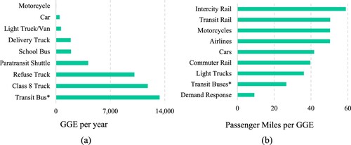
Urban public transport planning has attracted considerable attention from researchers and governments, who are exploring alternatives to mobility issues that could provide social, economic and environmental benefits. Millions of citizens around the world use public transport daily, and the accelerated increase in users caused by ever-increasing urban population growth is an important subject to consider. In addition, public transportation users are increasing faster than the population itself: the population has increased by 23% since 1995 in the USA, while ridership has increased by 28% (APTA 2020). Buses, including bus rapid transit (BRT) systems, are the most used mode of public transport worldwide, although they have the highest consumption rate of all land transportation options, as shown in Figure 1(a). Almost 68% of transit buses are regular 12 m buses (UITP 2019), which are often inefficient in terms of fuel economy because of their low passenger load rates (Figure 1b).

Figure 1. (a) Annual average of fuel consumption, where gasoline gallons equivalent (GGEs) denote the amount of combustible fuel (e.g. diesel or electricity) it takes to equal the energy contained in a gasoline gallon. (b) Transit buses that travel with few passengers have been shown to produce more greenhouse gas emissions per passenger mile than private cars (EPA 2020).

With millions of journeys being taken daily, public transport and especially transit buses are a great way to encourage commuters away from private cars, thus reducing road congestion and greenhouse gas (GHG) emissions. In addition, when dispatching the appropriate kind of bus to attend the ridership volume during different periods of the day, the transit of unfilled buses consuming unnecessary fuel is reduced. The most popular fuel used in the propulsion systems of buses is diesel, followed by diesel combined with additives or biodiesel (50% and 22%, respectively). Furthermore, in regular cities, bus fleets are normally composed of standard buses (comfort capacity of 75 and a maximum capacity of 100 pax), midibuses (comfort capacity of 55 and a maximum capacity of 75 pax) and minibuses (comfort capacity of 22 and a maximum capacity of 30 pax). The multi-objective formulation proposed herein is based on the importance of reducing the number of buses operating with low ridership, which are wasting fuel and unnecessarily increasing air pollution (i.e. GHG emissions), while reducing waiting times, safety and comfort, which are all desirable features from the passengers’ point of view.

This study focuses on the optimization of timetables that assign different bus types (i.e. different capacity, weight, power and fuel consumption) to cover a defined route, analysing its effects on GHG emissions when the number of transit vehicles is reduced, as well as the consequences in terms of degradation of quality of service (QoS). It also attempts to highlight the benefits of determining a timetable combining different types of vehicle, inspired by the suggestions made by Potter (2003) to prevent overloads and enhance vehicle utilization. The problem is mathematically modelled and called the multiple vehicle-types timetabling problem (MVTTP).

The contributions of this article are: (1) the definition of a new multi-objective combinatorial optimization problem to manage the fleet and schedule of buses in the framework of public transport for smart and sustainable cities, minimizing the environmental impact and the QoS; (2) the resolution of the problem with two multi-objective evolutionary algorithms (MOEAs), namely, the cellular genetic algorithm for multi-objective optimization (MOCell) and non-dominated sorting genetic algorithm-II (NSGA-II); (3) the design, implementation and evaluation of several evolutionary operators for the considered problem, as well as a thorough experiment to obtain the best configuration of the algorithms; (4) an exhaustive comparison between MOCell and NSGA-II; and, finally, (5) the generation of various timetables for a real-world scenario that assigns different kinds of buses to cover the daily demand on the route, reducing the carbon footprint while maintaining an acceptable QoS; the decision maker can choose the best one according to governmental restrictions.

The remainder of this article is structured as follows. Next, in Section 2, a brief analysis of the most relevant works on the topic is given. Section 3 states the problem definition and provides a detailed description of the mathematical model. Section 4 introduces MOEAs and some key concepts of multi-objective optimization. Section 5 describes the simulation methodology, analysing and discussing the experimental results. Finally, Section 6 concludes the article and briefly explores directions for future work.

2. Related works

Methods to address combinatorial problems such as the timetabling or bus dispatching problem can be classified into two principal classes. On the one hand, exact techniques can ensure that the global optimal solution is obtained. However, they are costly methods and therefore they usually can only be applied for small-sized problem instances (Ceder 2016). On the other hand, heuristic and metaheuristic algorithms are popular methods for finding high-quality approximations to the global optimum. They are more efficient and flexible than exact methods, allowing reasonably good solutions to be found with low computational effort.

2.1. Vehicle frequency and timetabling determination

Studies aiming to solve the bus dispatching problem usually address it by estimating the required vehicle frequency to set the timetable. Beginning with the Bus Scheduling Manual in 1947 (Rainville 1982), in the absence of computers or mathematical programs, some empirical or early methods appeared. For example, in 1967, a work presented by researchers at the University of Leeds supposes that a wrong early solution cannot be transformed into the correct one by heuristic enhancements (Wren 2004). Later, Newell (1971) suggests reducing the users’ waiting time, comparing a smoothed passenger arrival function with a set of vehicles with an assigned timetable, concluding that the large vehicle frequency fluctuates over time. Ceder (2016) collects and presents four methods to determine the vehicles’ frequency using the passenger demand (user load profile) and constraints defined by local authorities or regulators. An optimal timetable could be obtained by selecting a reference point based on peak passenger load.

Other studies have tackled transport planning problems (bus departure frequency and timetabling) using multi-objective optimization techniques. Kwan and Chang (2008) present a bi-objective formulation for a scheduling problem with conflicting goals: the required transfers and their associated cost minimization and the reduction of detriment caused by variations from a preliminary schedule. Hassold and Ceder (2014) solved a real instance in New Zealand, presenting important reductions in waiting times and unfilled space on the whole fleet. The authors developed a graph-inspired heuristic, which combines various schedules considering different vehicle types seeking the Pareto front. A more recent work uses the data provided by geolocalization sensors placed in the buses and information from the passengers’ transport cards to compute timetables using an improved version of NSGA-II. A bi-objective optimization model is proposed to reduce the total waiting time of passengers and the departure times of buses. The experiments were conducted using one bus line in Beijing to validate the approach (Tang et al. 2021).

In previous studies, a model was proposed focusing on operating costs that affect the service provider business and passenger benefits (Peña 2017; Peña et al. 2019). However, these works do not consider the environmental impact and its consequences. Griswold et al. (2017) proposed a solution to minimize costs, subject to restrictions on pollutant emissions, for a case study in Barcelona; they optimized the bus transit network design by adapting a classical model of continuum approximation considering the user costs (the time spent on accessing, waiting, transferring and riding) and costs related to maintenance and operation. Neither the bus frequency nor the heterogeneous fleet is considered.

2.2. Estimation of vehicle fuel consumption

Several relevant research articles have presented an energy and fuel consumption analysis of buses, some of them considering the notion introduced by Jiménez-Palacios (1999), known as vehicle specific power (VSP). The purpose is to determine the vehicle fuel consumption based on driving, road and transit conditions, combining the loads resulting from acceleration, rolling resistance, hill climbing and aerodynamic drag force, all divided by the vehicle mass in tons. For example, Frey et al. (2007) obtained information about the increment in average emission rates concerning raising VSP for transit buses (diesel and hydrogen) towards future combinations of transportation and emissions models.

In Yu and Li (2014), bus stops are taken into account to evaluate the bus emissions generated by the acceleration sequences of vehicles when approaching stops. Other techniques to compute fuel consumption were developed in various studies. Yu, Li, and Li (2016) stated, after real experiments on diesel buses, that the influence of passenger load on the GHG emissions becomes notable when travelling at 30 km/h or above (relatively high speed), while no apparent effect was perceived up to that speed.

Wang and Rakha (2017) use the Virginia Tech Comprehensive Power-based Fuel consumption Model (VT-CPFM) framework to enhance the estimation of bus fuel consumption, finding that the consumption rate is a concave function in terms of vehicle power. Yang and Liu (2020) apply genetic algorithms (GAs) to address the BRT dispatching problem considering the connections among the type of vehicle, passengers’ waiting time and fuel consumption. The authors present a mechanical model, similar to VSP, to express the energy consumption in various vehicles, considering engine features, vehicle and road characteristics, and driving modes. The average waiting time for users and the load factor are used to estimate the QoS.

This work uses a real instance to test the problem formulation, which considers two consecutive phases of public transport planning (vehicle frequency and scheduling) and the heuristic algorithm. It is formulated taking into account the conflicting objectives of the environmental impact of the bus’s operation and the QoS offered. A heterogeneous bus fleet is considered to compute the timetable, aiming to contribute to both objectives.

3. The multi-objective MVTTP model

Efficient and sustainable urban public transport systems are among the main challenges of the twenty-first century. Such systems involve three main participants, which have different purposes: (1) citizens, who are potential public transport users and expect more economical, efficient, secure, comfortable and environmentally friendly modes for daily mobility; (2) companies in the transportation sector, which aim to reduce operating costs and maximize profits under the regulations of local authorities; and (3) government, which defines policies to assure the quality of life, establishing mobility rules that satisfy their transportation requirements and mitigate environmental repercussions.

3.1. Problem description

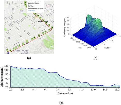
Ceder (2016) suggested four basic tasks, typically executed in sequence, to address a public transportation planning problem where users’ needs, economic constraints and environmental recommendations are considered. These tasks are route network design, timetable development, vehicle and crew scheduling. The MVTTP formulation considers that the network design cannot be modified. To achieve the second task, two activities were developed in sequence: the first is the frequency definition, and the second is the creation of the bus fleet timetable. Consequently, the bus stops are placed in a previously defined route map (Figure 2a), and the mobility data, information about the route condition (e.g. elevation profile), average vehicle speed, etc., are available. For the current work, passengers are counted in periods of 1 h (Figure 2b).

Figure 2. Route 217 Los Angeles. (a) Route map with stops markers and a maximum passenger load of 481 people in Fairfax/Rosewood between 17:00 and 18:00. (b) User demand ride-check data for 19 periods of 60 min for a total of 59 stops (Ceder 2016). (c) Route elevation profile with the highest gradient of 6% slope at 2.2 km (northbound). The data set can be downloaded from GitHub (https://github.com/davidpmorales/MVTTP).

MVTTP is defined as a multi-objective optimization problem (MOP) with the purpose of finding a proper distribution of a bus fleet , where $n$ is the number of vehicle types available and $b_i$ is the quantity of the $i$th type of vehicle ($\sum _{i=1}^n{b}_i$ is the whole fleet), with two conflicting goals. The first goal is to reduce the fuel consumption $(f_1)$ by means of reducing the number of buses driving with low capacity, and implicitly the GHG emissions generated by the vehicle used to cover a trip of a specific route $R$. The minimization of $f_1$ also contributes to a reduction in the operational costs (e.g. fuel, driver salary and regular maintenance), and improves road traffic flow by reducing unnecessary bus circulation and large unfilled vehicles wasting fuel and polluting the environment. The second goal is to minimize the unsatisfied user demand $(f_2)$, which that represents the QoS and implies a great experience regarding accessibility, safety and comfort. The latter is habitually correlated with the number of passengers onboard and the user waiting time.

3.2. MVTTP mathematical formulation

The MVTTP is formulated considering the objective functions $f_1$ and $f_2$, as follows:

Minimize (1) $f_1=\sum _{tp=1}^{L_{tp}}F{C}_{tp}$(1) and (2) $f_2=\sum _{tp=1}^{L_{tp}}UU{D}_{tp}$(2) where $F{C}_{tp}$ is the buses’ fuel consumption and $UU{D}_{tp}$ represents the unsatisfied user demand along a time period $tp$ ($L_{tp}$ is the last period of time).

Estimation of the fuel consumption for the selected buses to cover several trips during each $tp$ is based on the VSP, as follows: (3) $\begin{array}{rl}F{C}_{tp}& =\sum _{k\in BU{S}_{tp}}{\tau }_{tp}\ast {\beta }_k^i\ast VS{P}_k^i\end{array}$(3) (4) $\begin{array}{rl}VS{P}_k^i& =v_k^i\left(1.1\ast a_k^i+g\ast \sin \alpha +g\ast \phi \ast \cos \alpha +\frac{{\rho }_{\text{air}}{A}_k^i{C}_D}{2\ast m_k^i}v{{}_k^i}^2\right)\end{array}$(4) where ${\tau }_{tp}$ is the time (s) taken to traverse the route for the $k$th bus of a defined bus set $(BU{S}_{tp}\subset B)$. ${\beta }_k^i$ is the fuel consumption rate of a vehicle type $i$. $VS{P}_k^i$ in given in kW/ton; the vehicle speed and acceleration $v_k^i$ in m/s, and $a_k^i$ in m/s²; $\alpha$ is the angle of inclination (degrees); $\phi$ is the coefficient of rolling resistance; ${\rho }_{air}$ is the ambient air density; $C_D$ is the drag coefficient; $A_k^i$ is the vehicle frontal surface (m²),; and $m_k^i$ is the bus mass (tons). ${\rho }_{\text{air}}$ = 1.2 kg/m³ at 20°C and $g\ast \phi \ast \cos \alpha$ = 0.127, as a result of multiplying g = 9.807 m/s² (acceleration due to gravity) by 0.013 (the $\phi$ value for concrete/asphalt roads) and for roadways with a slope less than 30% ($\alpha$ = 17°), $\cos \alpha \approx 1$ with an error of less than $5\mathrm{\%}$ (Hao et al. 2014). The drag coefficient for buses varies between 0.60 and 0.70, depending on the exterior design and frontal area of the vehicle $A_k^i$. Different associations, e.g. ATUC in Spain, suggest that the average speed of a regular bus on a work day could be approximately 12 km/h (Morales and Gaspar 2016). Other studies, such as Oskarbski (2015), claim that the average speed of public transport is less than 30 km/h. Consequently, a static mass $(m_k^i)$ is assumed in this study for the different kinds of bus based on the lack of influence of ridership mass (Yu, Li, and Li 2016). (5) $VS{P}_k^i=v_k^i\ast (1.1\ast a_k^i+9.807\ast grade+0.127+0.00042\ast A_k^i\ast v{{}_k^i}^2\ast m{{}_k^i}^{-1})$(5) Function $f_2$ is subject to (6) $UU{D}_{tp}=\sum _{s\in R}max\left(U{D}_s^{tp}-L{F}_{tp}\ast \sum _{k\in BU{S}_{tp}}CA{P}_k^i,0\right)$(6) where the loss of QoS is represented by $UU{D}_{tp}$, as the passenger demand at bus stop $s$ $(U{D}_s^{tp})$ that exceeds the capacity of the set of buses $BU{S}_{tp}$, where $CA{P}_k^i$ is the capacity of each bus in $BU{S}_{tp}$ (buses used during time period tp). $R$ is the set of all bus stops $s$ making up the route. The desired occupancy percentage of the vehicles in period $tp$ is defined as the load factor, $0<L{F}_{tp}\le 1$, which should be less than or equal to the maximum occupancy permitted by local authorities, $L{F}_{tp}\le L{F}_{tp}^{max}$. $L{F}_{tp}$ can change during the operational time periods according to area characterizations, e.g. at peak hours the operator can admit major occupancy of vehicles owing to the higher levels of traffic congestion.

4. Multi-objective evolutionary algorithms (MOEAs)

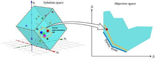
MOEAs are very useful tools for dealing with hard MOPs (Deb 2001), where the goal is to approximate the Pareto front as much as possible in terms of convergence and dispersion, with a large and diverse solution set being desirable. This set of solutions is called a Pareto approximation set (Figure 3).

Figure 3. Graphic representation of the solution space, objective space and Pareto front.

The present work considers two MOEAs, NSGA-II (Deb et al. 2002) and MOCell (Nebro et al. 2009). NSGA-II is probably the most well-known MOEA, and it has been applied before to optimize different problems related to sustainable public mobility, such as the optimization of the powertrain design in hybrid electric buses and vehicles (Ribau, Vieira, and Silva 2018; Wang et al. 2019), the optimization of the fuel cell power system (Kwan and Chang 2018), the planification/synchronization of bus lines and timetables (Khoo and Ong 2015; Wu et al. 2016) and other problems (Mercier, Poirion, and Désidéri 2019). Furthermore, MOCell has been shown to outperform NSGA-II on many benchmarks and real-world problems (Kar et al. 2019; Luna 2018; Nebro et al. 2009; Talasliuoglu 2021; Wen et al. 2020).

Both NSGA-II and MOCell are genetic algorithms. NSGA-II makes use of a panmictic population. In every generation, new individuals are generated using the genetic operators until the population size is doubled, then ranking (focused on dominance) and crowding (aiming at improving diversity) mechanisms are used to select the best individuals for the next generation.

The main feature of MOCell is the distribution of the population in a toroidal grid (Figure 4), with the aim of defining neighbourhoods for each individual, thus defining its mating pool (Alba and Dorronsoro 2008). The main idea behind this limitation is to produce a slow diffusion of genetic material over the population thanks to the overlaps between neighbourhoods, which enhances the exploration capabilities of the algorithm, while exploitation is promoted inside. MOCell holds an external repository containing the best non-dominated solutions found, and it feeds the population.

Figure 4. Reproduction steps in the cellular genetic algorithm for multi-objective optimization (MOCell) using spheres representing different solutions. The array attached to each sphere is the genotype of an individual, and its phenotype represents the departure times and vehicle type defined in the timetable computed by the proposed approach to solve the multiple vehicle-types timetabling problem (MVTTP).

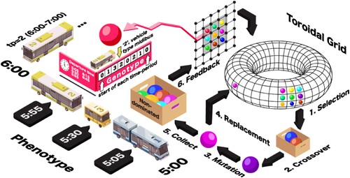
Figure 4 illustrates an instance of the proposed encoding of solutions (individuals’ genotype and phenotype) for a situation with three different types of buses, five scheduled trips and two time periods of one hour. The chromosome length is determined from a user demand study, conducted beforehand, using a frequency calculation method based on the load profile. $\overline{CAP}$ is the average capacities of the multiple vehicle types available, and it is used to calculate the dispatching frequency $(f_{tp})$, as follows: (7) $\begin{array}{rl}{f}_{tp}& =\text{max}\left(\frac{UD{A}_{tp}}{L{F}_{tp}\ast \overline{CAP}\ast L},\frac{U{D}_{tp}^{max}}{\overline{CAP}},f_{tp}^{min}\right)\end{array}$(7) (8) $\begin{array}{rl}UD{A}_{tp}& =\sum _{s\in R}U{D}_s^{tp}\ast {\ell }_s\end{array}$(8) (9) $\begin{array}{rl}L& =\sum _{s\in R}{\ell }_s\end{array}$(9) where $UD{A}_{tp}$ is the passenger-km area under the load curve and $U{D}_{tp}^{max}$ is the highest number of users at any stop $s\in R$ during $tp$; $l_s$ is the distance (km) between the stops $s$ and $s+1$, and the route span is $L$ (Ceder 2007). The distribution of zero markers cannot be consecutive because an important restriction made by local authorities’ is the minimum operating frequency $f_{tp}^{min}$, and every time period has the same duration (60 min), but it can be tuned depending on the total time spent (${\tau }_{tp}^R$) to cover the route, considering $f_{tp}^{min}$.

4.1. Population initialization

After calculating the operation frequency for each time period $(f_{tp})$, the structure (positions of the zero markers and each departure time) of the chromosome and size are defined. The initial population is constructed with individuals whose allele values are randomly assigned using integer numbers between 1 and $n$ (available vehicle types).

4.2. Fitness evaluation

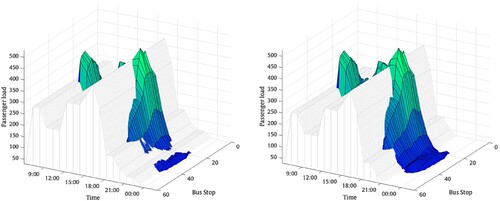
Solutions are evaluated as defined in Section 3.2. $f_1$ (Equation 1(1) $f_1=\sum _{tp=1}^{L_{tp}}F{C}_{tp}$(1) ) computes the fuel consumption and implicitly the GHG emissions covering all route departures. $f_2$ is a measure of the observed loss in QoS when passenger demand is not reached. In Figure 5, the pale grey surface represents the total fleet capacity while the darker (coloured) surface one is the user demand.

Figure 5. Example of unsatisfied user demand given two different vehicle assignments.

4.3. Evolutionary operators

4.3.1. Selection operator

The two parents are chosen by binary tournament, consisting of the random selection of two individuals from the population, from which the better one is chosen as a parent.

4.3.2. Crossover operators

In a natural process, crossover occurs between pairs of chromosomes by the exchange of genetic information between them with a probability $P_x$. In this work, five crossover operators adapted from versions extensively used in the literature are proposed, as follows.

Single-point and two-point crossover (SPX and TPX) are alternative versions of the traditional methods that consist of randomly choosing one (or two) zero-marker location(s) as the crossover point(s). In SPX, all the periods between the first and the selected zero-marker are taken from one parent. The rest of the genetic information is inherited from the second chromosome. In TPX, genetic information between the first crossover point and the second one is copied from one parent, and the remaining two parts of the chromosome are copied from the second parent.

The discrete crossover (DX) operator assigns the offspring genetic information from a random draw between the two parents (with probability $P_x^{DX}=0.5$). For each chromosome position of the first offspring, its value is inherited from the parent that wins the raffle. The process is repeated for a second offspring.

Uniform crossover (UX) is a process where the genetic information of the offspring (two new individuals) is the same as that of the given parents, but some positions are swapped probabilistically (with some probability $P_x^{UX}$). UX lets parents participate more at the gene level than to the whole time period, in contrast to SPX or TPX. Using the same procedure of UX but ensuring that half of the non-matching integer values are swapped, half uniform crossover (HUX) is the last proposed crossover operator, where it is possible to guarantee that the allele values from one parent that do not match with the second one must be swapped many times until they reach the Hamming distance, between the parents, divided by two.

4.3.3. Mutation operators

Mutation plays an essential role in the evolutionary process because it creates new individuals with at least one variation in their genetic information. It introduces slight random changes into the individual. Mutation happens during the course of evolution according to a probability $P_m$.

The proposed mutation operators are: uniform mutation (UM), which randomly chooses a subset of genes from the whole chromosome, the values of which are exchanged by new arbitrary values from a set of available vehicle types built randomly for each generation; one gene per period mutation (OGPPM), which randomly selects one position from each time-period subset in the chromosome, exchanging its values for different randomly selected ones; and reset period mutation (RPM), which randomly takes a whole time-period subset and replaces all its values with another possible integer value in a random way.

5. Experimental results

This section describes the parameter settings for the algorithms and the results of experimental analysis for a given user demand, using the data from a real bus route in Los Angeles city. This is a well-known instance that has been previously used to solve the proposed timetabling problem with some analytical and heuristic methods (Ceder 2007, 2016).

5.1. Performance metrics

The performance of MOEAs is evaluated using experimental tests, and various performance metrics have been introduced for this purpose. Metrics analyse mainly three aspects of a solution set (Riquelme, Von Lucken, and Baran 2015):

• The number of non-dominant solutions obtained (cardinality), which belong to the computed approximation Pareto set. Intuitively, a higher number of solutions is preferred.

• The convergence, defined as the distance between the Pareto front approximation $(P_F^{\text{approx}})$ produced by the stochastic algorithm and the Pareto front $(P_F^{\text{true}})$. To evaluate this, the ϵ-indicator ($I_{\epsilon }$) metric is used, which determines a factor ϵ that estimates how much worse one set of solutions is than another (Zitzler et al. 2003). The ϵ-indicator employs $P_F^{\text{true}}$, which is unknown for the proposed instance. However, an artificial Pareto front, $P_F^{\text{artificial}}$, as a representation of $P_F^{\text{true}}$, is constructed by joining all the non-dominated solutions sets computed by the two MOEAs in all conducted experiments. Using that significant number of solutions establishes a more extensive approximation to the Pareto front, as proposed by Dorronsoro (2014).

• The diversity, as a measure of the dispersion of solutions along the computed front. The spread ($I$) metric proposed by Deb et al. (2002) is used to evaluate diversity, and the hypervolume $(I_{HV})$ metric (Zitzler and Thiele 1999) is used to assess diversity and convergence together.

Likewise, in addition to the performance for the previously mentioned metrics to compare the solution sets of the two studied algorithms, two-set coverage $(I_{TSC})$ is used to evaluate the relative coverage between two sets (Zitzler, Deb, and Thiele 2000).

Before applying these performance metrics, the evaluated solution set is normalized with the extreme values for every objective function. The normalization helps to avoid some bias due to the differences in the order of magnitude of the two objective functions (unsatisfied user demand and fuel consumption).

5.2. Experimental methodology

To obtain confident results for evaluating the quality of the obtained solutions and the performance of the algorithm, 30 independent runs of the proposed algorithms were executed, using several parameter configurations. For each run, 10,000 fitness evaluations were made (100 generations using 100 individuals per population), and 1500 different algorithm configurations were tested in total.

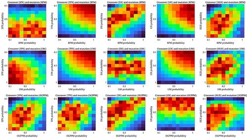
The hypervolume metric was used to compare the performance and analyse the impact of different settings on the quality of the resulting solution sets, since it allows the convergence and dispersion to be validated simultaneously. A Shapiro–Wilk test was applied to assess the statistical significance of the experimental results (Shapiro and Wilk 1965). The test confirmed that 90% of the experimental results displayed a normal distribution. Then, a non-parametric statistical test was implemented (Friedman test); this uses the recurrent analysis of variance by ranks to define the best combination of parameters that significantly affect the algorithm’s performance and provides higher quality hypervolume results (Sheskin 2003). Figure 6 shows the Friedman rank for the 1500 tested configurations, where each heatmap is clustered by the evolutionary operators’ couples and their considered probabilities.

Figure 6. Ranking of the configurations of the studied algorithms using the Friedman test according to $I_{HV}$ performance (dark red represents better rank value). SPX = single-point crossover; TPX = single-point crossover; DX = discrete crossover; UX = uniform crossover; HUX = half uniform crossover; RPM = reset period mutation; UM = uniform mutation; OGPPM = one gene per period mutation.

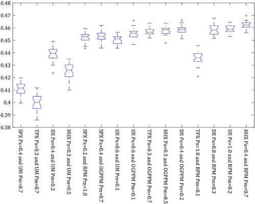
The results shown in Figure 6 are chosen as the best selection of crossover and mutation operators and their probabilities $(P_m$ and $P_x)$. Fifteen algorithm configurations are selected and 30 independent runs for each one are compared, obtaining a significant statistical difference with a confidence level of 95% [χ²(14) = 398, p = 2.2e⁻¹⁶]. To select only one as the best parameter configuration, a Friedman test was implemented, as suggested by García et al. (2009). The combination of HUX with $P_x=0.4$ and RPM with $P_m=0.7$ obtained the best rank. Figure 7 shows the hypervolume behaviour from the independent runs of the MOCell algorithm for each one of the 15 selected combinations of the genetic operators and their respective probabilities. It is essential to consider that the greater the hypervolume value, the better the efficiency on convergence and dispersion.

Figure 7. $I_{HV}$ comparison for the 15 different parameter configurations of the cellular genetic algorithm for multi-objective optimization (MOCell). SPX = single-point crossover; TPX = single-point crossover; DX = discrete crossover; UX = uniform crossover; HUX = half uniform crossover; RPM = reset period mutation; UM = uniform mutation; OGPPM = one gene per period mutation.

The chosen configuration is the one offering the best performance, and it uses HUX and RPM operators with probabilities of 0.7 and 0.4, respectively. After extensive experimentation, the parameter settings used for the MOCell-based algorithm are summarized in Tables 1–2. The same configuration was also adopted for NSGA-II.

Table 1. Summary of related research on timetabling and bus scheduling.

	Real instances	Sustainability	Time scheduling	Vehicle frequency	Heterogeneous fleet	Empirical/mathematical models	Heuristics	Multi-objective
Rainville (1947, 1982)	X	X	✓	✓	X	✓	X	X
Newell (1971)	X	X	✓	X	X	✓	X	X
Kwan and Chang (2008)	X	X	✓	✓	X	X	X	✓
Ceder (2016)	✓	X	✓	✓	X	X	✓	X
Ceder (2016)	X	X	✓	✓	X	X	✓	X
Griswold et al. (2017)	✓	X	X	X	X	X	✓	X
Peña (2017)	✓	X	✓	✓	✓	X	X	✓
Peña et al. (2019)	✓	X	✓	✓	✓	X	✓	✓
Yang and Liu (2020)	✓	✓	X	X	✓	X	✓	✓
Tang et al. (2021)	✓	X	✓	X	X	X	✓	✓

Table 2. Parameter configuration of the multi-objective evolutionary algorithms (MOEAs).

	Parameter value/method
Parameter	MOCell	NSGA-II
Termination condition	10,000 fitness evaluations	2000 generations
Population size	100	200
Neighbourhood	C9	N/A
Selection method	Binary tournament	Binary tournament
Crossover operator	HUX	HUX
$P_x$	40%	40%
Mutation operator	RPM	RPM
$P_m$	70%	70%
Feedback set size	20	N/A

Note: MOCell = cellular genetic algorithm for multi-objective optimization; NSGA-II = non-dominated sorting genetic algorithm-II; HUX = half uniform crossover; RPM = reset period mutation; N/A = not applicable.

5.3. Results and discussion

Thirty independent runs of MOCell and NSGA-II were performed to solve the problem. The evolution of the hypervolume metric during the MOCell optimization process for the 30 test runs is shown in Figure 8(a). It is possible to observe an $I_{HV}^{\text{MOCell}}$ maximum value of 0.4846, 0.4729 on average, in the last generation. Furthermore, $I_{HV}^{\text{MOCell}}$ improves similarly in each run, exhibiting a stable behaviour for the studied parameter configuration.

Figure 8. (a) Hypervolume performance metric convergence for the cellular genetic algorithm for multi-objective optimization (MOCell) in each independent run. (b) Comparison of the best approximation fronts computed by both algorithms. NSGA-II = non-dominated sorting genetic algorithm-II.

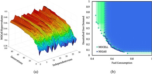
The best Pareto front approximations found by the two algorithms are compared in Figure 8(b). The best approximation reported by NSGA-II has a hypervolume value of 0.4263. Therefore, the MOCell approach is clearly, given that the best $I_{HV}^{\text{NSGAII}}$ value is lower than the average hypervolume of MOCell for the same input data. Figure 8 highlights MOCell features, such as the feedback from an external archive and the utilization of crowding distance as the density estimator, promoting elitism and exploration in the solution space with the aim of finding more skilled individuals, increasing the spread along the approximation front.

Table 3 presents the results obtained by the two algorithms on all considered performance metrics. Results marked with an asterisk indicate the best performing algorithm for each metric, where the obtained p-value in the comparison is less than 0.05. The NSGA-II results exhibit better behaviour for the cardinality performance, having a higher number of non-dominated solutions than MOCell in the reported Pareto approximations. However, MOCell outperforms NSGA-II in terms of convergence and diversity of the Pareto front, therefore providing better solutions.

Table 3. Metric performance results considering 30 independent runs for each algorithm.

Metric	$I_{\mathrm{\Delta }}^{\text{NSGAII}}$	$I_{\mathrm{\Delta }}^{\text{MOCell}}$	$I_{HV}^{\text{NSGAII}}$	$I_{HV}^{\text{MOCell}}$	$I_{\epsilon }^{\text{NSGAII}}$	$I_{\epsilon }^{\text{MOCell}}$	$I_{TSC}(P_F^{NSGAII},P_F^{MOCell})$	$I_{TSC}(P_F^{MOCell},P_F^{NSGAII})$
Min.	0.5853	0.5072*	0.4233	0.4598	4.3780	2.1983*	0.1538	0
Mean	0.7467	0.6398*	0.4242	0.4729*	6.3360	3.2980*	0.3278*	0.1438
Max.	0.9550	0.7869	0.4263	0.4846*	7.7654	4.7811	0.4791*	0.4008

Note: *Best performing algorithm for each metric (p-value for the comparison < 0.05).

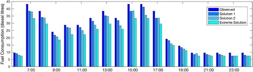
Figure 9 shows the fuel consumption of four possible solutions: two obtained with MOCell, an extreme solution with the smallest buses, and the actual schedule observed, using buses of the same type in each trip for actual timetables on the LA 217 bus route. For each time period, the computed fuel consumption by the MOCell approach is 13% lower on average than the observed timetable, not only representing an important reduction of carbon dioxide (approximately 150 kg/day), but also, when using minibuses or midibuses, supporting reductions in traffic and operating costs, given the high value of the fuel. On average, MOCell solutions use 55.3% fewer traditional city buses (standard buses) than the assigned schedule for the LA route, combining the total allocation with midibuses (36%) and small vehicles (20% of the trips use minibuses) for lower ridership periods. However, the QoS (unsatisfied user demand level) worsens as the fuel consumption decreases.

Figure 9. Comparison of fuel consumption rates from two non-dominated solutions, considering a heterogeneous bus fleet, an extreme solution with only minibuses and the observed vehicle dispatch using only standard buses for the 217 bus route in Los Angeles.

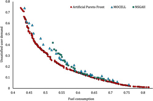
Furthermore, $P_F^{\text{artificial}}$ (created after 45,000 experiments in this work) is compared in Figure 10 with the best approximations computed by the MOEAs, $P_F^{\text{NSGAII}}$ and $P_F^{\text{MOCell}}$. It can be seen that $P_F^{\text{NSGAII}}$ concentrates its solutions in the central region, finding complications to generate solutions out of this region. However, $P_F^{\text{MOCell}}$ covers better the space of non-dominated solutions. Solutions in $P_F^{\text{NSGAII}}$ dominate almost half of the solutions in $P_F^{\text{MOCell}}$. NSGA-II provides approximately 33% more solutions with better fitness than MOCell, on average. However, using the same configuration, MOCell is able to explore the solution space in a better way than NSGA-II.

Figure 10. Best solution sets for the non-dominated sorting genetic algorithm-II (NSGA-II) and cellular genetic algorithm for multi-objective optimization (MOCell) (square and triangle marks, respectively). Dot marks represent the artificial Pareto front built using the best individuals of the 45,000 algorithm executions performed in this work.

Summarizing, the results of NSGA-II provide more solutions that dominate those of MOCell in a specific region of the objective space (better results for cardinality and $I_{TSC}$). Otherwise, MOCell produces a sufficiently good approximation to the true Pareto front, while preserving diversity (better results for $I_{\epsilon }$, $I_{\mathrm{\Delta }}$ and $I_{HV}$).

The decision maker is usually interested in trade-offs based on policies that are typically framed by local authorities’ restrictions or dynamic situations such as weather conditions or holidays. The outcome of the MOEAs is a set of different solutions, none of which is better than another. However, the solutions can be changed dynamically, e.g. by prioritizing a high QoS during peak hours or saving fuel consumption in periods with low demand.

6. Conclusions

This article introduces a new multi-objective combinatorial optimization problem, called MVTTP, in the framework of public transport in smart cities. The problem is to select appropriate types of buses and their timetables to cover the daily needs of the routes while minimizing the environmental impact and maximizing the QoS. The problem is mathematically modelled to propose a representation and appropriate operators to solve it with evolutionary algorithms.

The problem is solved with MOCell and NSGA-II, two state-of-the-art multi-objective optimization algorithms. The two algorithms are exhaustively compared, according to their performance, when solving a real-world instance of the city of Los Angeles. The experimental analysis demonstrates that the solutions provided by the two metaheuristics can improve the actual bus operation mode, reducing the fuel consumption and improving the QoS. It also guarantees the level of service defined by government entities. MOCell was found to outperform NSGA-II for the considered metrics with 95% confidence interval, providing a wide range of trade-off timetables according to the regulations and policies of local authorities.

Defining the MVTTP as a multi-objective problem allows decision makers to choose among solutions of similar quality but with different features, depending on the needs a specific time. For example, near the peak hours, the QoS can be significantly improved by selecting the solution with the largest bus in the last trip before the peak hour. Solutions found in this study allow the LA 217 bus route to be enhanced by choosing the appropriate bus to use every time, from a heterogeneous fleet, in terms of both fuel consumption (and inherently the GHG emissions) and the QoS offered to users, and thus encouraging public transport use.

Directions for future work include considering real-time traffic information to enhance vehicle distribution and produce flexible and adaptable solutions for each period. In addition, to explore diverse dynamic situations, it is possible to use the knowledge of the problem to adjust the crossover or mutation operators, to find suitable schedules that use a heterogeneous fleet. Another prospect for future work is the possibility of including hybrid, compressed natural gas and electric vehicles. The impact of GHG reduction will be considered under the right conditions, improving the QoS not only for passengers but also for other people; for example, providing an opportunity to reduce noise in urban areas.

Contributions

All authors have conceived, designed and performed the experiments and analysed the data. The authors worked on this article together and all authors have read and approved the final manuscript.

Acknowledgements

This project was partially funded by the Spanish Ministerio de Ciencia, Innovación y Universidades and the ERDF [contract RTI2018-100754-B-I00] (iSUN project), ERDF [project FEDER-UCA18-108393] (OPTIMALE), and Junta de Andalucía and ERDF (GENIUS) [project P18-2399].

Disclosure statement

No potential conflict of interest was reported by the authors.

Additional information

Funding

This project was partially funded by the Spanish Ministerio de Ciencia, Innovación y Universidades and the ERDF [contract RTI2018-100754-B-I00] (iSUN project), ERDF [project FEDER-UCA18-108393] (OPTIMALE), and Junta de Andalucía and ERDF (GENIUS) [project P18-2399].

References

- Alba, E., and B. Dorronsoro. 2008. Cellular Genetic Algorithms. Operations Research/Computer Science Interfaces Series (Vol. 42). New York: Springer.
- APTA. 2020. 2020 Public Transportation Fact Book. American Public Transportation Association. https://www.apta.com/wp-content/uploads/APTA-2020-Fact-Book.pdf.
- Ceder, A. 2007. Public Transit Planning and Operation: Theory, Modeling and Practice. 1st ed. Oxford: Elsevier.
- Ceder, A. 2016. Public Transit Planning and Operation: Modeling, Practice and Behavior. 2nd ed. Boca Raton, FL: CRC Press.
- Deb, K. 2001. Multi-objective Optimization Using Evolutionary Algorithms. New York: John Wiley and Sons.
- Deb, K., A. Pratap, S. Agarwal, and T. Meyarivan. 2002. “A Fast and Elitist Multiobjective Genetic Algorithm: NSGA-II.” IEEE Transactions on Evolutionary Computation 6 (2): 182–197.
- Dorronsoro, B. 2014. Evolutionary Algorithms for Mobile Ad Hoc Networks. Hoboken, NJ: John Wiley and Sons.
- EPA. 2020. Inventory of US Greenhouse Gas Emissions and Sinks. US Environmental Protection Agency.
- Frey, H. Christopher, Nagui M. Rouphail, Haibo Zhai, Tiago L. Farias, and Gonçalo A. Gonçalves. 2007. “Comparing Real-World Fuel Consumption for Diesel- and Hydrogen-Fueled Transit Buses and Implication for Emissions.” Transportation Research Part D: Transport and Environment 12 (4): 281–291.
- García, S., A. Fernández, J. Luengo, and F. Herrera. 2009. “A Study of Statistical Techniques and Performance Measures for Genetics-Based Machine Learning: Accuracy and Interpretability.” Soft Computing 13 (10): 959–977.
- Griswold, J. B., Tal Sztainer, Jinwoo Lee, Samer Madanat, and Arpad Horvath. 2017. “Optimizing Urban Bus Transit Network Design Can Lead to Greenhouse Gas Emissions Reduction.” Frontiers in Built Environment 3: 1–7.
- Hao, H., Yong Geng, Hewu Wang, and Minggao Ouyang. 2014. “Regional Disparity of Urban Passenger Transport Associated GHG (Greenhouse gas) Emissions in China: A Review.” Energy 68: 783–793.
- Hassold, S., and A. A. Ceder. 2014. “Public Transport Vehicle Scheduling Featuring Multiple Vehicle Types.” Transportation Research Part B: Methodological 67: 129–143.
- Jiménez-Palacios, J. L. 1999. “Understanding and Quantifying Motor Vehicle Emissions with Vehicle Specific Power and Tuneable Infrared Laser Differential Absorption Spectrometer Remote Sensing.” PhD thesis, MIT.
- Kar, M. B., S. Kar, S. Guo, X. Li, and S. Majumder. 2019. “A New Bi-objective Fuzzy Portfolio Selection Model and its Solution Through Evolutionary Algorithms.” Soft Computing 23: 4367–4381.
- Khoo, H. L., and G. P. Ong. 2015. “Bi-objective Optimization Approach for Exclusive Bus Lane Scheduling Design.” Journal of Computing in Civil Engineering 29 (5): 04014056:1–04014056:16.
- Kwan, C. M., and C. S. Chang. 2008. “Timetable Synchronization of Mass Rapid Transit System Using Multiobjective Evolutionary Approach.” IEEE Transactions on Systems, Man, and Cybernetics, Part C (Applications and Reviews) 38 (5): 636–648.
- Luna, F. 2018. “Addressing the 5G Cell Switch-off Problem with a Multi-objective Cellular Genetic Algorithm.” 2018 IEEE 5G world forum, 422–426.
- Mercier, Q., F. Poirion, and J. A. Désidéri. 2019. “Non-convex Multiobjective Optimization Under Uncertainty: A Descent Algorithm. Application to Sandwich Plate Design and Reliability.” Engineering Optimization 51 (5): 733–752.
- Morales, C., and I. Gaspar. 2016. El 80% del tiempo que un autobús está parado es por culpa de los semáforos. https://www.atuc.es/noticias.
- Nebro, A. J., J. J. Durillo, F. Luna, B. Dorronsoro, and E. Alba. 2009. “MOCell: A Cellular Genetic Algorithm for Multiobjective Optimization.” International Journal of Intelligent Systems 24 (7): 726–746.
- Newell, G. F. 1971. “Dispatching Policies for a Transportation Route.” Transportation Science 5 (1): 91–105.
- Oskarbski, J. 2015. “Estimating the Average Speed of Public Transport Vehicles Based on Traffic Control System Data.” 2015 international conference on models and technologies for intelligent transportation systems, 287–293.
- Peña, D. 2017. “Multiobjective Optimization of Greenhouse Gas Emissions Enhancing the Quality of Service for Urban Public Transport Timetabling.” 4th international conference on engineering and telecommunication, 114–118.
- Peña, D., Andrei Tchernykh, Sergio Nesmachnow, Renzo Massobrio, Alexander Feoktistov, Igor Bychkov, Gleb Radchenko, Alexander Yu. Drozdov, and Sergey N. Garichev. 2019. “Operating Cost and Quality of Service Optimization for Multi-Vehicle-Type Timetabling for Urban Bus Systems.” Journal of Parallel and Distributed Computing 133: 272–285.
- Potter, S. 2003. “Transport Energy and Emissions: Urban Public Transport.” In Handbook of Transport and the Environment, edited by D. A. Hensher, and K. J. Button, 247–262. Emerald Group Publishing Limited, Bingley.
- Rainville, W. S. 1982. Bus Scheduling Manual: Traffic Checking and Schedule Preparation. UMTA in cooperation with APTA, DOT-1-8223 (August 1947, reprinted July 1982).
- Ribau, J. P., S. M. Vieira, and C. M. Silva. 2018. “Selecting Sustainable Electric Bus Powertrains Using Multipreference Evolutionary Algorithms.” International Journal of Sustainable Transportation 12 (8): 592–612.
- Riquelme, N., C. Von Lucken, and B. Baran. 2015. “Performance Metrics in Multi-Objective Optimization.” 2015 Latin American computing conference (CLEI), 1–11.
- Shapiro, S. S., and M. B. Wilk. 1965. “An Analysis of Variance Test for Normality (Complete Samples).” Biometrika 52 (3/4): 591–611.
- Sheskin, D. J. 2003. Handbook of Parametric and Nonparametric Statistical Procedures. 3rd ed. New York: Chapman and Hall.
- Talasliuoglu, T. 2021. “A Comparative Study of Multi-objective Evolutionary Metaheuristics for Lattice Girder Design Optimization.” Structural Engineering and Mechanics 77 (3): 417–439.
- Tang, J., Yifan Yang, Wei Hao, Fang Liu, and Yinhai Wang. 2021. “A Data-Driven Timetable Optimization of Urban Bus Line Based on Multi-objective Genetic Algorithm.” IEEE Transactions on Intelligent Transportation Systems 22 (4): 2417–2429.
- UITP. 2019. Global Bus Survey Report of International Association of Public Transport. https://www.uitp.org/sites/default/files/cck-focus-papers-files/Statistics Brief_Global bus survey %28003%29.pdf.
- Wang, Z., Yang Cai, Yuping Zeng, and Jie Yu. 2019. “Multi-objective Optimization for Plug-In 4WD Hybrid Electric Vehicle Powertrain.” Applied Sciences 9 (19): 4068:1–4068:21.
- Wang, J., and H. A. Rakha. 2017. “Convex Fuel Consumption Model for Diesel and Hybrid Buses.” Transportation Research Record: Journal of the Transportation Research Board 2647 (1): 50–60.
- Wen, T., Haotian Liu, Luxin Lin, Bin Wang, Jigong Hou, Chuanbo Huang, Ting Pan, and Yu Du. 2020. “Multiswarm Artificial Bee Colony Algorithm Based on Spark Cloud Computing Platform for Medical Image Registration.” Computer Methods and Programs in Biomedicine 192: 105432:1–105432:10.
- Wren, A. 2004. Scheduling Vehicles and Their Drivers (Issue April). Leeds, UK: School of Computing, University of Leeds.
- Wu, Y., H. Yang, J. Tang, and Y. Yu. 2016. “Multi-objective Re-synchronizing of Bus Timetable: Model, Complexity and Solution.” Transportation Research Part C: Emerging Technologies 67: 149–168.
- Yang, X., and L. Liu. 2020. “A Multi-objective Bus Rapid Transit Energy Saving Dispatching Optimization Considering Multiple Types of Vehicles.” IEEE Access 8: 79459–79471.
- Yu, Q., and T. Li. 2014. “Evaluation of Bus Emissions Generated Near Bus Stops.” Atmospheric Environment 85: 195–203.
- Yu, Q., T. Li, and H. Li. 2016. “Improving Urban Bus Emission and Fuel Consumption Modelling by Incorporating Passenger Load Factor for Real World Driving.” Applied Energy 161: 101–111.
- Zitzler, E., K. Deb, and L. Thiele. 2000. “Comparison of Multiobjective Evolutionary Algorithms: Empirical Results.” Evolutionary Computation 8 (2): 173–195.
- Zitzler, E., and L. Thiele. 1999. “Multiobjective Evolutionary Algorithms: A Comparative Case Study and the Strength Pareto Approach.” IEEE Transactions on Evolutionary Computation 3 (4): 257–271.
- Zitzler, E., L. Thiele, M. Laumanns, C. M. Fonseca, and V. G. da Fonseca. 2003. “Performance Assessment of Multiobjective Optimizers: An Analysis and Review.” IEEE Transactions on Evolutionary Computation 7 (2): 117–132.