A new job priority rule for the NEH-based heuristic to minimize makespan in permutation flowshops

Abstract

The permutation flowshop scheduling problem is a vital production management concern of industries such as electronic product manufacturing and integrated circuit fabrication. In many studies, jobs are prioritized independently according to their features or properties. This article develops a new perspective by introducing the self-attention mechanism into scheduling for the first time. The job similarities are characterized by the dot-product of processing time matrices and taken as job priorities. Based on this idea, a new priority rule denoted by PR_SAT is proposed, and a heuristic named NEHLJP2 is presented with makespan minimization. The computational results with the Taillard and VRF benchmarks and 640 random instances demonstrate that the new priority rule and heuristic dominate the existing ones at a nominal cost of computation time.

KEYWORDS:

• Priority rule
• job similarity
• flowshop scheduling
• heuristic

1. Introduction

The flowshop scheduling problem, along with its variants (Gao, Chen, and Deng 2013; Choi, Kim, and Lee 2005; Alfieri 2009), has been extensively studied as it is employed across various industries. For example, a fabrication factory may use a large amount of customized machinery to produce one or many similar goods. In practice, an extra constraint is generally included and studied, ensuring that the job routings are all the same through the machines and are not allowed to change. This constraint is derived from either technical requirements or the simplification of management work. A real-world case is presented by Erseven et al. (2019), in which a local company that produces apparel and garments has to schedule several jobs with different processing times on each station. Nevertheless, the job sequences on each station are kept the same. The scheduling for this type of production is defined as the permutation flowshop scheduling problem (PFSP) in the research field.

For PFSPs, heuristic algorithms are developed to obtain an optimal or a near-optimal schedule in a short time. Priority rules or dispatching rules, as one typical heuristic, have been studied extensively for decades in both academia and industry (Tay and Ho 2008). The rule for job scheduling is commonly defined as the dispatching rule, while the rule to provide initial solutions for the composite heuristic is called the priority rule. Many simple dispatching rules, including the shortest processing time (SPT), longest processing time (LPT), earliest due date (EDD) and first come, first served (FCFS) rules, are used directly for job scheduling. The composite dispatching rules are commonly developed by including several job features or properties, such as job due date, job arrival time, job processing time, job weight and remaining job processing time. For example, Xiong et al. (2017) developed four priority rules considering operation slack time for a dynamic jobshop scheduling problem. Vallada, Ruiz, and Minella (2008) evaluated several dispatching rules concerning job due date, slack time and processing time, with the criterion of total tardiness. Job tardiness, due date and processing time are included in the dispatching rules for the flexible jobshop scheduling problem (Kianfar, Fatemi Ghomi, and Karimi 2009).

In general, the job features are carefully selected, and the dispatching rule is designed for a given problem. The advantage of this idea is that the addition or deletion of a job will not change the relative positions of the remaining jobs (Koulamas and Panwalkar 2018). However, the job position in the sequence should be a relative instead of an absolute parameter, and it should depend on the interrelationship among jobs. This article proposes a new perspective by calculating job similarity with a self-attention mechanism for developing a priority rule, and the PFSP is used for validation. To investigate the effectiveness of the new rule, it is implemented with the NEH heuristic (Nawaz, Enscore, and Ham 1983) as well as existing tie-breaking rules (Dong, Huang, and Chen 2008; Kalczynski and Kamburowski 2008; Liu, Jin, and Price 2017a), in terms of makespan minimization.

The remainder of this article is structured as follows. In Section 2, the related literature is reviewed. The terminology and performance measures are given in Section 3. Section 4 provides the background and physical meaning of the new perspective associated with the new priority rule. In Section 5, test cases and computational results are presented, demonstrating the newly proposed priority rule and heuristic effectiveness. Finally, conclusions are presented in Section 6.

2. Literature review

One priority rule is constructed with two elements for effective job scheduling: the indicators based on job features and the sorting method. The indicators are the main factors considered in the priority rule and are used for job differentiation. Jayamohan and Rajendran (2004) proposed priority rules based on operation due date, job slack time, job processing time, etc., for minimizing penalties for job flowtime and tardiness. The adjusted processing times and job completion time are considered for the weighted total job completion time. Weng and Ren (2006) developed a composite priority rule based on job slack time and queue length for the dynamic jobshop scheduling problem while minimizing mean job tardiness. Sha et al. (2006) considered the length of the queue in the dispatching rule while considering the rework of defective products. Swaminathan et al. (2007) developed the EDD-based dispatching rule for dynamic flowshop with uncertain processing times for minimizing total weighted tardiness. Natarajan et al. (2007) designed several dispatching rules concerning job finishing time, arrival time and starting time for the assembly jobshop with the criteria of weighted flowtime and job tardiness. To deal with the blocking flowshop scheduling problem, Wang et al. (2012) developed an initial job priority rule considering job average processing time and standard deviation for the three-phase algorithm. To schedule the new orders in the dynamic flowshop, Liu, Jin, and Price (2017b) developed a priority rule for the match-up and real-time (MR) strategy by assigning different weights to job processing times.

Along with the indicators in priority rules, the sorting method determines the job positions. Framinan, Leisten, and Rajendran (2003) summarized eight different sorting criteria, namely DECR, INCR, VALLEY, HILL, HI/HILO, HI/LOHI, LO/HILO and LO/LOHI. The DECR means that jobs are sorted according to the decreasing indicator values, while the INCR is according to the increasing indicator values. The VALLEY sets low indicator values in the middle of the initial sequence and high figures at the beginning and the end, whereas HILL is the opposite, with high indicator values in the middle of the initial sequence and low figures at the beginning and the end. The sorting methods HI/HILO, HI/LOHI, LO/HILO and LO/LOHI select low and high indicator values alternately. Swaminathan et al. (2007) used a composite ranking scheme in which three criteria are used simultaneously and the sum of rank positions is adopted. Therefore, by combining different job indicators and sorting methods, priority or dispatching rules can be generated for various problems.

As a typical combination optimization problem, the PFSP has been thoroughly studied, and the priority rules have been applied in many algorithms (Nagano and Moccellin 2002). The optimization criteria for the PFSP are commonly makespan, flowtime or machine idletime (Framinan, Leisten, and Rajendran 2003; Liu, Jin, and Price 2016), to satisfy various requirements from production practice. The PFSP is an NP-hard problem with the makespan criterion (Rinnooy Kan 1976) and flowtime criterion (Framinan, Leisten, and Ruiz-Usano 2005), so that many heuristics are designed to obtain optimal or near-optimal solutions in a short time. For the makespan criterion, the NEH heuristic is commonly regarded as the most effective (Dong, Huang, and Chen 2008; Kalczynski and Kamburowski 2009), and many variants have been developed for various criteria (Nagano and Moccellin 2002; Liu, Jin, and Price 2016). Many new NEH improvements have also been developed in terms of tie-breaking rules, such as those presented by Sharma, Sharma, and Sharma (2021), Sauvey and Sauer (2020), Baskar and Xavior (2021), Benavides et al. (2018) and Wu et al. (2021).

Regarding the makespan minimization, the original priority rule of the NEH heuristic uses the LPT dispatching rule. The N&M algorithm (Nagano and Moccellin 2002) is a variant of the NEH heuristic in which jobs are arranged according to the total job processing times and the maximum lower bound of the job waiting times between machines. Framinan, Leisten, and Rajendran (2003) tested 177 different initial job priority rules, and the results show that the LPT rule achieves the best makespan minimization performance. In the NEH-D heuristic (Dong, Huang, and Chen 2008), the average and standard deviation of job processing times are considered, and the non-increasing order of job indicators is chosen. For the NEHKK1 (Kalczynski and Kamburowski 2008) and NEHKK2 (Kalczynski and Kamburowski 2009) heuristics, different weights are allocated to job processing times according to their position in the flow line. Ribas, Companys, and Tort-Martorell (2010) tested four priority rules with the NEH-insertion method, including rules from NEHKK1, N&M, LPT and a random job sequence. In the NEHLJP1 heuristic (Liu, Jin, and Price 2017a), the job processing times are assumed as a set of discrete random numbers, and the first, second and third moments, namely, the average, standard deviation and skewness, are included. The fourth moment of the job processing times is included and tested for the bi-criteria of makespan and idletime for the PFSPs (Liu, Jin, and Price 2016). Note that the non-increasing order of indicators is commonly adopted in the priority rules for the makespan criterion. All of the above priority rules are constructed by selecting appropriate job features, and the interrelationships between jobs are not considered.

In summary, many studies assume that jobs are sorted independently based on their features, and job priority rules are developed with sorting methods for the given problems. A full consideration of job interrelationships should be further studied to differentiate jobs precisely. In this article, the job similarities are studied, allowing a new perspective to be developed on constructing a new priority rule.

3. Terminology and measures of performance

In the permutation flowshop environment, n jobs are assumed to be available at time zero, to be processed on m machines in the same order. Machines can only process one job at a time, and failures are not considered in this article. Buffers between machines are assumed to be infinite. Denoted by $t_{i,j}$, the processing time of job i on machine j, including the machine set-up time, is known and deterministic. Job pre-emption is not allowed. To understand the various rules in this article, the terminology used in herein is listed in Table 1.

Table 1. Terminology.

Notation	Description
n	Number of jobs
m	Number of machines
i	Index for a job, 1 ≤ i ≤ n
[i]	ith job in the job sequence
j, k	Index for a machine, 1 ≤ j, k ≤ m
t[i],k	Processing time of ith job on machine k
Q, K, V	Query matrix, key matrix, value matrix
${\mathit{d}}_{\mathit{K}}$	Dimension of matrix K
C[i],k	Completion time of ith job on machine k
T	Job processing time matrix
ST	Standardized job processing time matrix

The makespan of the schedule is given by (1) $Makespan=C_{\left[n\right],m}$(1) where (2) $C_{\left[i\right],j}=max\left(C_{\left[i-1\right],j},C_{\left[i\right],j-1}\right)+t_{\left[i\right],j}i=1,\dots ,n;j=1,\dots ,m$(2) (3) $C_{\left[1\right],0}=0,C_{\left[0\right],1}=0$(3)

4. New perspective

4.1. Self-attention mechanism

To calculate the similarity of jobs, the self-attention mechanism from the deep learning network (Vaswani et al. 2017; Kool, van Hoof, and Welling 2018; Bengio, Lodi, and Prouvost 2018) is introduced into scheduling. To provide an explicit introduction, the scaled dot-product attention mechanism (Vaswani et al. 2017) is presented first; this can be formulated as follows: (4) $A\left(\mathit{Q},\mathit{K},\mathit{V}\right)=softmax\left(\frac{\mathit{Q}\times {\mathit{K}}^T}{\sqrt{d_{\mathit{K}}}}\right)\times \mathit{V}$(4) where $\mathit{Q}$ is the query matrix, $\mathit{K}$ is the key matrix, ${\mathit{K}}^T$ is the transpose of $\mathit{K}$, $\mathit{V}$ is the value matrix, and $1/\sqrt{d_{\mathit{K}}}$ is the scaling factor, with $d_{\mathit{K}}$ as the dimension of $\mathit{K}$. $\mathit{Q}$ is a set of vectors to calculate attention for, and $\mathit{K}$ is a set of vectors to calculate attention against. The result of the dot-product multiplication shows how attended each query is against $\mathit{K}$, which are used as weights to matrix $\mathit{V}$. The Softmax function performs the following transform on m numbers: (5) $softmax\left(x_j\right)=\frac{{\text{e}}^{x_k}}{{\sum }_{k=1}^m{\text{e}}^{x_k}},j,k=1,\dots ,m$(5)

From Equation (5)(5) $softmax\left(x_j\right)=\frac{{\text{e}}^{x_k}}{{\sum }_{k=1}^m{\text{e}}^{x_k}},j,k=1,\dots ,m$(5) , it can be seen that the result of the attention mechanism is a convex combination of the row vectors of the value matrix $\mathit{V}$, where the weights assigned to each row are determined by the dot-product of matrix $\mathit{Q}$ with matrix $\mathit{K}$.

When the query matrix $\mathit{Q}$, the key matrix $\mathit{K}$ and the value matrix $\mathit{V}$ are set to be the same, this is called the self-attention mechanism, as shown in Equation (6)(6) $A\left(\mathit{Q},\mathit{Q},\mathit{Q}\right)=softmax\left(\frac{\mathit{Q}\times {\mathit{Q}}^T}{\sqrt{d_{\mathit{K}}}}\right)\times \mathit{Q}$(6) : (6) $A\left(\mathit{Q},\mathit{Q},\mathit{Q}\right)=softmax\left(\frac{\mathit{Q}\times {\mathit{Q}}^T}{\sqrt{d_{\mathit{K}}}}\right)\times \mathit{Q}$(6)

Herein, the dot-product of the matrices is used to calculate the similarities among the rows of the matrix $\mathit{Q}$ and then taken as weights for each element of $\mathit{Q}$.

To introduce the self-attention mechanism into PFSP scheduling, the matrix as the arithmetic object should be built. In this article, each job is deemed to be a vector of m elements, representing the processing times with m machines. All n jobs are grouped, constructing the (n × m)-dimensional processing time matrix, denoted by $\mathit{T}$. Each row of T consists of the processing times of the corresponding job on all machines. As the jobs with similar processing patterns may affect the scheduling of a job more strongly than those with a different pattern, the similarity between two rows can be viewed as the influence between the related jobs. In this sense, the result of the dot-product is another matrix, where the (jk)th element represents the influence of job j’s features on job k. Then, the similarities are assigned as weights to each row of $Q$ after composition with the Softmax function. The Softmax function can turn arbitrary real values into probabilities. An extra dimension for adjustment, $1/\sqrt{d_{\mathit{K}}}$, is added to prevent the inner product from becoming too large.

If the self-attention mechanism is implemented with the job processing time matrix, the Softmax function will convert the dot-product of $\mathit{T}$s into a job similarity matrix, which is then used as a weighting parameter for matrix $\mathit{T}$.

4.2. New priority rule

For the PFSPs, the processing times of n jobs with m machines are generally assumed to be larger than 1 (Taillard 1993; Vallada, Ruiz, and Framinan 2015). As a result, the dot-product of the processing time matrix will be large, which will increase the risk of large variance. Two strategies are employed to prevent this problem. First, the processing time matrix is standardized so that the matrix element values are mapped to [0, 1], denoted by ${\mathit{T}}_{\mathit{S}}$. Secondly, a scaling factor is introduced after the dot-product of the processing time matrices. In the new rule, ${\mathit{S}}_{\mathit{R}}$ is formulated as (7) ${\mathit{S}}_{\mathit{R}}=softmax({\mathit{T}}_{\mathit{S}}\times {{\mathit{T}}_{\mathit{S}}}^T\times \alpha {)}^T\times \mathit{T}$(7) where $\mathit{T}$ is the processing time matrix; $\alpha ={\log }_3\left(n\right)+\frac{200}{n}\ast lo{g}_6\left(m\right)$ for n < 100, else$\alpha ={\log }_6\left(n\right)+\frac{100}{n}\ast \text{lo}{\text{g}}_6\left(m\right)$ for n ≥ 100. The row sum of $S_R$ is taken as the job priorities. The rationality behind the scaling factor setting is that ${\mathit{S}}_{\mathit{R}}$ depends on n and m differently. The result of ${\mathit{T}}_{\mathit{S}}\times {{\mathit{T}}_{\mathit{S}}}^T$ is an n × n matrix in which each element is the sum of m product values of two job processing times. Therefore, the impact of m on the Softmax function is larger than n, and it should be limited. Besides, a nonlinear function is used to control the scale of n or m further, and the log function is selected based on preliminary tests. Note that the specified hyperparameters of the scaling factor are based on the authors’ two-year calculation and heuristic design experience. Readers are welcome to optimize them further.

The (ij)th element of ${\mathit{T}}_{\mathit{S}}\times {{\mathit{T}}_{\mathit{S}}}^T$ measures the similarity between job i and job j, considering the processing times with all machines. Treating this as a multiplicative weight, each row of the matrix ${\mathit{S}}_{\mathit{R}}$ is a weighted sum of all jobs, which measures the influence of the target job on all of the jobs. The bigger it is, the larger the impact of this job will be. That is, this job is likely to have a significant impact on other jobs.

The result of the self-attention mechanism is a matrix with size n × m, and its row sum is used as a job sorting indicator. Regarding the sorting method, many existing rules adopt the non-increasing sorting method for the makespan criterion owing to its optimality rates, such as rules from NEH, NEHKK1, NEHKK2, NEH-D and NEHLJP1. In this article, the non-increasing order is implemented with the above indicator for the makespan criterion, and the new priority rule is denoted by PR_SAT.

By combining PR_SAT and the tie-breaking rule developed by the authors (Liu, Jin, and Price 2017a), TB_LJP1, a new heuristic denoted by NEHLJP2, is presented.

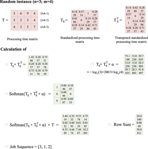
4.3. Numerical example

A numerical example is demonstrated with calculation details as follows, to improve the understanding of the new priority rule. As illustrated in Figure 1, three jobs are to be processed in a four-machine permutation flowshop. The processing times of job 1 with machines 1, 2, 3 and 4 are 3, 6, 1 and 4, respectively. The processing time matrix $\mathit{T}$ can be formulated if all job processing times are grouped and the size of $\mathit{T}$ is 3 × 4. The results of each step are given in detail below.

Figure 1. Sample demonstration of PR_SAT with four digits shown.

4.4. Computational complexity and running time comparison

As matrix ${\mathit{T}}_{\mathit{S}}$ is of size n × m and matrix ${{\mathit{T}}_{\mathit{S}}}^T$, m × n, the multiplication ${\mathit{T}}_{\mathit{S}}\times {{\mathit{T}}_{\mathit{S}}}^T$ takes O(n²m) arithmetic operations. When carrying out the Softmax computation, the complexity depends on the value of the numbers involved. Assuming that the element value of ${\mathit{T}}_{\mathit{S}}$ is upper bounded by some constant, the complexity of the Softmax function is O(n²). Finally, the matrix $softmax({\mathit{T}}_{\mathit{S}}\times {{\mathit{T}}_{\mathit{S}}}^T\times \alpha {)}^T$ is of size n × n, and the matrix multiplication with $\mathit{T}$ will take O(n²m) operations. Above all, the complexity upper bound for the computation of ${\mathit{S}}_{\mathit{R}}$ is O(n²m), as well as the priority rule of PR_SAT.

Table 2 summarizes the computational complexities of some existing priority rules for the NEH heuristic. The current rules, such as PR_AVG, PR_STD and PR_SKE, share the same complexity of O(nlog(n)), while for PR_SAT, it is O(n²m). Since the complexity of NEH insertion is O(n²m), all of these rules implemented with the NEH heuristic will achieve O(n²m).

Table 2. Complexities and running times (in seconds) of priority rules.

Priority rule	Computational complexity	Computational complexity with NEH heuristic	Computational time with NEH heuristic
PRAVG	O(nlog(n))	O(n^2m)	1.3721
PRSTD	O(nlog(n))	O(n^2m)	1.3821
PRSKE	O(nlog(n))	O(n^2m)	1.3840
PRSAT	O(n^2m)	O(n^2m)	1.3900

The average computation times of each rule implemented with the NEH heuristic are also listed in Table 2, and the Taillard (Taillard 1993) and VRF (Vallada, Ruiz, and Framinan 2015) instances are used for the test. All priority rules and the NEH heuristic are coded with MATLAB^® R2020a and run on an Intel Core CPU i9-9900 K computer with 32 GB memory. It can be seen that with both benchmarks, the original priority rule PR_AVG with the NEH heuristic needs the least running time, followed by PR_STD. The rule PR_SKE requires more running time than both PR_AVG and PR_STD, since an extra indicator of job skewness is considered. For the rule of PR_SAT, the running time is slightly larger than for PR_SKE, although it has the largest computational complexity. This is because the complexities of all NEH-based heuristics are the same, and priority rules have a minor impact on the overall running time.

5. Experimental results

To validate the effectiveness of the new priority rule PR_SAT and the heuristic NEHLJP2, two classic benchmarks, namely Taillard (Taillard 1993) and VRF (Vallada, Ruiz, and Framinan 2015), are employed simultaneously, associated with one new set of random instances. In the Taillard benchmark, there are 120 instances, with n = 20, 50, 100, 200, 500, and m = 5, 10, 20. For the VRF benchmark, the small instance set includes 240 instances, with n = 10, 20, 30, 40, 50, 60, 70, 80, and m = 5, 10, 15, 20. In the large instance set, 240 instances are included, with n = 100, 200, 300, 400, 500, 600, 700, 800, and m = 20, 40, 60. To further test the new priority rule and the new heuristic performance, 640 instances are randomly generated, including 320 small instances and 320 large instances. For small instances, the number of jobs is assumed to be 20, 50, 100, 200, and the number of machines is 5, 10, 15, 20. Regarding the large random instances, n is defined as 300, 400, 500, 600, and m as 20, 30, 40, 50. Twenty instances are generated for each problem combination. Job processing times are independently drawn from the uniform distribution U({1, 2, … , 99}). Therefore, in this article, 1240 instances are used for performance validation.

To demonstrate the performance of each rule, the relative percentage deviation (RPD) is used. The RPD is calculated as follows: $RPD=\frac{HS-UB}{UB}\times 100\mathrm{\%}$ where $HS$ is the objective function value obtained by a specific algorithm on a given test instance, and $UB$ is the upper bound of each instance. The average relative percentage deviation (ARPD) on all instances is used to demonstrate the algorithm’s overall performance.

In the following subsections, the performance of the new priority rule is first verified. Two different verification scenarios are defined. One is that the new priority rule is implemented with the NEH heuristic directly. The second scenario is that the tie-breaking rules are adopted and run with the new priority rule to fully validate the performance and compatibility of the priority rule. Note that, to confirm the effectiveness of the new priority rule, some existing priority rules for the NEH heuristic are referenced, including the original rule PR_AVG from the NEH heuristic, PR_STD from NEH-D (Dong, Huang, and Chen 2008) and PR_SKE from NEHLJP1 (Liu, Jin, and Price 2017a).

Next, the performance of the heuristic NEHLJP2 is validated. Two independent test scenarios are set as well. First, NEHLJP2 is tested directly with three groups of instances. The existing heuristics NEH, NEHKK1, NEHKK2, NEH-D, NEHFF and NEHLJP1 are taken as references. Secondly, the iterated greedy (IG) algorithm (Ruiz and Stützle 2007) is selected for further performance tests by taking the heuristic result as its initial solution.

For a fair performance comparison, all algorithms are coded in MATLAB R2020a and run on an Intel Core CPU i9-9900 K computer with 32 GB memory.

5.1. Performance of the new priority rule

Table 3 shows the ARPD values of some existing priority rules when the makespan is minimized with the Taillard benchmark. The PR_SAT achieves the best ARPD value, 3.0488, followed by PR_SKE, PR_STD and PR_AVG. Performance improvements of 8.30%, 5.46% and 0.38% are realized by the new priority rule compared to PR_SKE, PR_STD and PR_AVG. Moreover, the PR_SAT rule has the best performance on six out of 12 problems, namely, the 20 × 5, 50 × 10, 50 × 20, 100 × 10, 200 × 10 and 500 × 20 problems. PR_SKE outperforms the others on four out of 12 problems.

Table 3. Average relative percentage deviation (ARPD) values of priority rules with the Taillard benchmark.

Problem	PRAVG	PRSTD	PRSKE	PRSAT
20 × 5	3.3003	2.7033	2.7081	2.0692
20 × 10	4.6011	4.0836	3.6837	4.3153
20 × 20	3.7309	3.8156	2.9135	3.4086
50 × 5	0.7272	0.8934	0.8785	0.7365
50 × 10	5.0729	4.9038	4.8435	4.6620
50 × 20	6.6481	6.1209	6.4194	5.8110
100 × 5	0.5272	0.4107	0.5381	0.5392
100 × 10	2.2150	2.1558	2.2411	1.9955
100 × 20	5.3446	5.6526	4.9883	5.5720
200 × 10	1.2579	1.2700	1.2428	1.2038
200 × 20	4.4076	4.5685	4.1449	4.2095
500 × 20	2.0661	2.1206	2.1231	2.0632
AVG	3.3249	3.2249	3.0604	3.0488

Note: The bold numbers indicate the best ARPD value for each problem.

The results with VRF instances are shown in Table 4. The priority rule PR_SAT is at the first level among all priority rules, achieving 3.4442 in ARPD, followed by PR_SKE, PR_STD and PR_AVG. Concerning the best ARPD value for each problem, PR_SAT performs best on 17 out of 48 problems, followed by PR_SKE on 16 out of 48 problems, PR_STD on 11 out of 48 problems and PR_AVG on four out of 48 problems.

Table 4. Average relative percentage deviation (ARPD) values of priority rules with the VRF benchmark.

Problem		PRAVG		PRSTD		PRSKE		PRSAT
S	L	S	L	S	L	S	L	S	L
10 × 5	100 × 20	2.1770	5.7082	1.5143	5.6140	1.5143	5.4432	1.9680	5.6298
10 × 10	100 × 40	1.6287	5.6673	1.4638	5.3144	1.4638	5.2475	0.9213	5.1475
10 × 15	100 × 60	1.5350	4.9486	2.1749	4.5114	2.2727	4.6964	1.3003	4.5155
10 × 20	200 × 20	1.9862	4.2314	1.5209	4.0399	1.6236	4.1258	1.7036	4.1337
20 × 5	200 × 40	1.5148	4.7117	2.7570	4.6569	2.8233	4.5563	2.6556	4.6701
20 × 10	200 × 60	4.8243	4.5546	4.9284	4.3540	4.8048	4.4515	5.4074	4.2635
20 × 15	300 × 20	4.3294	2.9960	3.9327	3.0308	3.8918	2.9978	3.7619	2.9221
20 × 20	300 × 40	4.1238	4.0818	3.5003	3.9008	3.5080	3.9738	3.6833	3.8249
30 × 5	300 × 60	1.4344	3.9339	1.6444	3.9090	1.5385	3.8545	1.0805	3.9670
30 × 10	400 × 20	5.2625	2.5811	5.4576	2.4564	4.7270	2.4664	5.2170	2.2708
30 × 15	400 × 40	5.8253	3.6605	5.4355	3.5092	5.2418	3.5723	4.7821	3.6053
30 × 20	400 × 60	5.4073	3.5597	5.4901	3.4693	5.5667	3.3630	5.0454	3.4127
40 × 5	500 × 20	1.0933	2.2742	0.7877	2.2282	0.9342	2.0026	0.8256	2.0062
40 × 10	500 × 40	4.9687	3.1976	4.5226	3.1091	4.1287	2.9958	4.1702	3.1324
40 × 15	500 × 60	6.0473	3.1151	5.8657	3.2046	5.7359	3.1046	5.6719	3.1057
40 × 20	600 × 20	5.1422	1.5704	5.2885	1.6425	5.3785	1.6078	5.6131	1.5925
50 × 5	600 × 40	0.5457	3.1346	0.8184	2.9847	0.7972	2.9652	0.6898	2.9080
50 × 10	600 × 60	4.5811	2.9344	4.4499	2.9386	4.2603	2.9132	4.0605	2.9106
50 × 15	700 × 20	6.5187	1.4001	6.9031	1.2345	6.2121	1.3010	6.5083	1.3593
50 × 20	700 × 40	5.9649	2.7725	6.0049	2.6036	5.6999	2.6494	5.9506	2.6664
60 × 5	700 × 60	0.8930	2.7511	0.4807	2.7086	0.5494	2.6876	0.5298	2.8340
60 × 10	800 × 20	3.9574	1.2309	3.9434	1.1529	4.3885	1.1316	4.4398	1.1643
60 × 15	800 × 40	5.7865	2.4312	5.9082	2.5158	5.9541	2.3955	6.1118	2.3914
60 × 20	800 × 60	6.4519	2.7068	6.4188	2.6739	6.5737	2.5730	6.1420	2.6472
AVG(S)	AVG(L)	3.8333	3.3397	3.8005	3.2401	3.7329	3.2115	3.6767	3.2117
AVG		3.5865		3.5203		3.4722		3.4442

Note: The bold numbers indicate the best ARPD value for each problem.

Table 5 presents the results of priority rules with random instances. PR_SAT achieves the best overall performance in terms of small and large instances. Primarily, it outperforms the other reference priority rules on 10 out of 16 problems.

Table 5. Average relative percentage deviation (ARPD) values of priority rules with random instances.

Problem		PRAVG		PRSTD		PRSKE		PRSAT
S	L	S	L	S	L	S	L	S	L
20 × 5	300 × 20	2.6133	3.1970	2.8006	3.1922	2.6347	3.1560	2.5781	3.1150
50 × 5	400 × 20	0.4618	2.3425	0.5972	2.2092	0.5652	2.1990	0.4915	2.1464
100 × 5	500 × 20	0.4482	1.6746	0.4126	1.6943	0.5140	1.7369	0.4056	1.7262
200 × 5	600 × 20	0.0893	1.2870	0.0912	1.2825	0.0849	1.2669	0.0962	1.2557
20 × 10	300 × 30	11.7908	6.5728	11.2344	6.5677	11.2553	6.5030	11.6699	6.6416
50 × 10	400 × 30	5.8826	5.3787	5.0210	5.1953	4.9574	5.3613	5.2399	5.2123
100 × 10	500 × 30	2.1018	4.3253	2.3423	4.1338	2.4941	4.2765	2.2897	4.2504
200 × 10	600 × 30	0.7368	3.7635	0.7808	3.6122	0.8804	3.6163	0.8100	3.5761
20 × 15	300 × 40	18.2276	10.4727	18.7569	10.5655	18.7338	10.4852	17.9277	10.4529
50 × 15	400 × 40	10.5968	8.5139	10.8416	8.4951	10.3960	8.3841	10.5458	8.3077
100 × 15	500 × 40	5.4712	6.9128	5.4782	6.7879	5.2154	6.8746	5.4407	6.7612
200 × 15	600 × 40	2.4463	5.8325	2.3892	5.8001	2.4385	5.8462	2.4615	5.7701
20 × 20	300 × 50	20.8783	14.0372	20.7264	13.8968	20.6798	13.7746	20.7577	13.8780
50 × 20	400 × 50	14.9448	10.7375	14.8821	10.5771	15.0273	10.6063	14.9176	10.5283
100 × 20	500 × 50	9.2058	9.8535	9.0389	9.8039	9.2329	9.7708	8.9855	9.7835
200 × 20	600 × 50	4.7412	8.2794	4.4960	8.2174	4.5572	8.2207	4.6530	8.2647
AVG(S)	AVG(L)	6.9148	6.4488	6.8681	6.3769	6.8542	6.3799	6.8294	6.3544
AVG		6.6818		6.6225		6.6170		6.5919

Note: The bold numbers indicate the best ARPD value for each problem.

To check whether the ARPD differences in priority rules are significant, a paired sample t-test was conducted with Taillard, VRF and randomly generated instances. As shown in Table 6, significant differences between PR_SAT, PR_SKE, PR_STD and PR_AVG can be observed, with p < 0.05. Note that PR_SAT and PR_SKE are significantly better than PR_STD, but there is no significant performance difference between PR_SAT and PR_SKE. This is because the performance of the existing priority rules is excellent, and it becomes harder to propose a new priority rule that can outperform the existing ones significantly. However, the contribution of developing a priority rule still exists, in that significantly better results can be obtained by combining it with other heuristics or metaheuristics, as demonstrated in Sections 5.3 and 5.5.

Table 6. Paired sample t-test results of priority rules, with 95% confidence intervals (CIs).

Pairs	Mean	SEM	CI lower	CI upper	T	Sig.
PRSAT–PRSKE	−0.02494	0.02542	−0.07481	0.02493	−0.981	0.327
PRSAT–PRSTD	−0.06231	0.02460	−0.11057	−0.01405	−2.533	0.011
PRSAT–PRAVG	−0.12822	0.02637	−0.17995	−0.07649	−4.863	0.000
PRSKE–PRSTD	−0.03737	0.01857	−0.07379	−0.00095	−2.013	0.044
PRSKE–PRAVG	−0.10327	0.02572	−0.15373	−0.05282	−4.016	0.000
PRSTD–PRAVG	−0.06590	0.02578	−0.11648	−0.01533	−2.557	0.011

5.2. Compatibility of the new priority rule

To further test the PR_SAT rule, it is implemented with the tie-breaking rules from NEHKK1, NEHKK2, NEH-D, FF (Fernandez-Viagas and Framinan 2014) and NEHLJP1. In addition, the above existing priority rules are referenced for comparison. Therefore, there are four priority rules and five tie-breaking rules included, and 20 different combinations are tested with different benchmarks.

The results of each combination with the Taillard benchmark are shown in Figure 2. It can be seen that PR_SAT works best with the tie-breaking rules from NEHKK1, NEH-D, NEHFF and NEHLJP1, but not NEHKK2. Specifically, with the NEHKK1, NEH-D, NEHFF and NEHLJP1 tie-breaking rules, PR_SAT achieves the best performance compared to other priority rules. Also, PR_SAT is the best with the NEHLJP1 tie-breaking rule, reaching 2.7025 in terms of ARPD value. Figure 3 shows the results of each combination with the VRF benchmark. Again, PR_SAT offers better performance than the other priority rules on five out of five tie-breaking rules.

Figure 2. Average relative percentage deviation (ARPD) values of each combination with the Taillard benchmark.

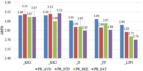
Figure 3. Average relative percentage deviation (ARPD) values of each combination with the VRF benchmark.

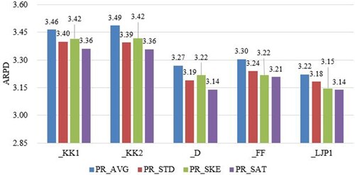
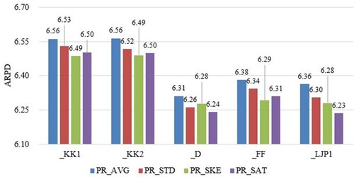
Figure 4 illustrates the performance of different combinations with randomly generated instances. It can be seen that PR_SAT obtains the best performance with the NEHLJP1 tie-breaking rule. To conclude, PR_SAT is compatible with the tie-breaking rules of NEHKK1, NEHKK2, NEH-D, NEHFF and NEHLJP1.

Figure 4. Average relative percentage deviation (ARPD) values of each combination with random instances.

5.3. Performance of NEHLJP2

In this section, the performance of NEHLJP2 is tested. To conduct a fair comparison, the existing NEH-based heuristics, NEH, NEHKK1, NEHKK2, NEH-D and NEHLJP1 are referenced and compared, and the ARPD value is taken as the performance measure.

Table 7 shows the ARPD values of each heuristic with Taillard instances. NEHLJP2 obtains the best ARPD performance, with an ARPD value of 2.7025, and 1.87% performance improvement is achieved compared to NEHLJP1, 6.98% compared to NEH-D, 13.16% compared to NEHKK2, 14.23% compared to NEHKK1 and 18.72% compared to NEH. Also, NEHLJP2 can achieve the best performance on five out of 12 problems, followed by NEHLJP1 on four out of 12 problems, NEHKK2 on two out of 12 problems and NEH-D on one out of 12 problems.

Table 7. Average relative percentage deviation (ARPD) values of heuristics with the Taillard benchmark.

Problem	NEH	NEHKK1	NEHKK2	NEH-D	NEHLJP1	NEHLJP2
20 × 5	3.3003	2.8094	2.4786	2.8131	2.2848	2.1126
20 × 10	4.6011	4.4343	4.1710	3.7525	3.6664	3.5120
20 × 20	3.7309	3.3368	3.5738	3.6443	3.0607	3.1608
50 × 5	0.7272	0.6674	0.4360	0.7333	0.6602	0.6679
50 × 10	5.0729	5.4620	5.3781	4.6623	4.2932	3.9270
50 × 20	6.6481	6.2473	6.2239	5.8119	6.0431	6.1841
100 × 5	0.5272	0.4126	0.2194	0.4012	0.3211	0.3812
100 × 10	2.2150	1.7780	2.2780	1.6984	1.7073	1.5878
100 × 20	5.3446	5.2323	5.3177	4.9812	4.8839	4.5075
200 × 10	1.2579	1.3206	1.0118	0.9553	0.8911	0.9772
200 × 20	4.4076	4.1656	4.2480	3.7534	3.6910	3.7359
500 × 20	2.0661	1.9459	2.0089	1.6575	1.5468	1.6757
AVG	3.3249	3.1510	3.1121	2.9054	2.7541	2.7025

Note: The bold numbers indicate the best ARPD value for each problem.

Similar results can be obtained with the VRF benchmark, as shown in Table 8. NEHLJP2 has the best overall ARPD value of 3.1382, and 0.27% performance improvement is achieved compared to NEHLJP1, 1.64% compared to NEH-D, 10.37% compared to NEHKK2, 9.34% compared to NEHKK1 and 12.50% compared to NEH. NEHLJP1 generates the best performance on most problems, 19 out of 48, followed by NEHLJP2, NEH-D, NEHKK2 and NEHKK1 with VRF instances.

Table 8. Average relative percentage deviation (ARPD) values of heuristics with the VRF benchmark.

Problem		NEH		NEHKK1		NEHKK2		NEH-D		NEHLJP1		NEHLJP2
S	L	S	L	S	L	S	L	S	L	S	L	S	L
10 × 5	100 × 20	2.1770	5.7082	1.9954	5.3690	2.3412	5.7003	1.2646	5.2459	1.4414	5.2850	1.4255	5.0683
10 × 10	100 × 40	1.6287	5.6673	1.5929	5.4581	2.3933	5.4233	1.8833	5.2658	1.5399	5.1963	0.9046	5.1251
10 × 15	100 × 60	1.5350	4.9486	1.4778	4.7182	1.8648	4.8567	2.1266	4.5138	2.2467	4.6291	1.1338	4.6717
10 × 20	200 × 20	1.9862	4.2314	1.5355	4.1779	1.4972	4.0003	1.8114	3.6594	1.8248	3.4960	1.6976	3.5751
20 × 5	200 × 40	1.5148	4.7117	1.1317	4.4928	2.4347	4.7561	2.9566	4.3431	2.7220	4.2135	1.9211	4.2234
20 × 10	200 × 60	4.8243	4.5546	5.0731	4.3045	4.7716	4.3117	4.9641	4.1730	4.7214	4.1932	4.6562	4.1202
20 × 15	300 × 20	4.3294	2.9960	4.2336	2.8512	4.1042	2.8226	3.8244	2.3824	3.8118	2.5957	3.9118	2.3267
20 × 20	300 × 40	4.1238	4.0818	3.9135	3.8045	4.2150	3.9920	3.3212	3.6017	3.2234	3.4274	3.4336	3.5821
30 × 5	300 × 60	1.4344	3.9339	0.9202	3.8432	1.0658	4.2362	1.1501	3.8414	0.8135	3.5638	0.8677	3.7462
30 × 10	400 × 20	5.2625	2.5811	5.0895	2.3858	5.2228	2.2119	4.7568	1.8894	4.4250	1.7879	4.6956	1.8379
30 × 15	400 × 40	5.8253	3.6605	6.0200	3.6961	5.5326	3.6024	4.5283	3.0835	5.1106	3.1780	4.6191	3.1727
30 × 20	400 × 60	5.4073	3.5597	5.4441	3.4220	5.6074	3.4874	5.1421	3.1640	5.3840	3.0865	5.4808	3.1843
40 × 5	500 × 20	1.0933	2.2742	0.6075	1.8386	0.4521	1.7332	0.7363	1.6065	0.5671	1.5856	0.6945	1.4272
40 × 10	500 × 40	4.9687	3.1976	4.7794	3.0863	5.0128	3.0218	4.0448	2.5616	4.1006	2.6859	4.1762	2.6561
40 × 15	500 × 60	6.0473	3.1151	6.1389	3.0943	6.3276	3.1860	5.2956	3.0083	5.3318	2.8267	5.2055	2.8523
40 × 20	600 × 20	5.1422	1.5704	5.3471	1.5027	5.3712	1.5190	5.1399	1.2663	5.1421	1.2056	5.1258	1.2111
50 × 5	600 × 40	0.5457	3.1346	0.4515	3.0043	0.3682	2.8788	0.3932	2.4839	0.4284	2.5057	0.4979	2.3920
50 × 10	600 × 60	4.5811	2.9344	4.2967	2.8618	3.4804	2.9419	3.7836	2.5282	3.4417	2.5996	3.5537	2.5468
50 × 15	700 × 20	6.5187	1.4001	6.3646	1.3297	6.1933	1.1124	5.5257	0.9408	5.6965	0.9339	6.2776	0.9895
50 × 20	700 × 40	5.9649	2.7725	6.3823	2.6841	6.1045	2.4539	5.8866	2.2262	5.1876	2.1400	5.9072	2.1574
60 × 5	700 × 60	0.8930	2.7511	0.7698	2.6815	0.1826	2.7639	0.4321	2.3524	0.4516	2.3336	0.4102	2.3573
60 × 10	800 × 20	3.9574	1.2309	4.0634	1.1349	4.0209	0.9519	3.3223	0.8780	3.3474	0.8463	3.6389	0.8550
60 × 15	800 × 40	5.7865	2.4312	5.6851	2.4356	5.9614	2.3185	5.8156	2.0221	5.4828	2.0001	5.7337	1.9735
60 × 20	800 × 60	6.4519	2.7068	6.0846	2.5804	6.6798	2.5649	5.6515	2.3561	6.0172	2.2670	6.3158	2.2977
AVG(S)	AVG(L)	3.8333	3.3397	3.7249	3.1982	3.8002	3.2020	3.4899	2.8914	3.4358	2.8576	3.4285	2.8479
AVG		3.5865		3.4616		3.5011		3.1906		3.1467		3.1382

Note: The bold numbers indicate the best ARPD value for each problem.

The heuristic results with 640 randomly generated instances are shown in Table 9. Overall, the new heuristic NEHLJP2 demonstrates the best solution quality compared to existing heuristics, with the lowest ARPD values in terms of small and large instances. NEH-D and NEHLJP1 are located at the second level of heuristic performance. Similarly, NEHLJP2, NEHLJP1 and NEH-D generate the best ARPD values for different problems. It can be concluded that NEHLJP2 shows a robust capability for developing high-quality solutions.

Table 9. Average relative percentage deviation (ARPD) values of heuristics with random instances.

Problem		NEH		NEHKK1		NEHKK2		NEH-D		NEHLJP1		NEHLJP2
S	L	S	L	S	L	S	L	S	L	S	L	S	L
20 × 5	300 × 20	2.6133	3.1970	2.5738	3.0479	2.5684	2.9174	2.6185	2.7200	2.4985	2.6498	2.5264	2.5515
50 × 5	400 × 20	0.4618	2.3425	0.3548	2.1715	0.3546	2.0814	0.4191	1.8707	0.4121	1.8867	0.3818	1.7724
100 × 5	500 × 20	0.4482	1.6746	0.3524	1.4921	0.3714	1.4887	0.3756	1.3973	0.3170	1.3131	0.3144	1.3704
200 × 5	600 × 20	0.0893	1.2870	0.0642	1.2187	0.0762	1.1745	0.0668	1.0263	0.0634	1.0110	0.0723	1.0217
20 × 10	300 × 30	11.7908	6.5728	11.7668	6.4826	11.8093	6.4101	10.8384	6.0335	11.0577	6.1753	11.4733	6.0066
50 × 10	400 × 30	5.8826	5.3787	5.0829	5.1073	5.0406	5.1588	4.9599	4.7989	4.8535	4.7790	4.3501	4.6616
100 × 10	500 × 30	2.1018	4.3253	2.0482	4.2233	2.0307	4.1023	2.0579	3.7600	1.9581	3.6762	1.9263	3.6675
200 × 10	600 × 30	0.7368	3.7635	0.7196	3.5205	0.7430	3.4170	0.6697	3.1364	0.6699	3.1602	0.7106	3.1053
20 × 15	300 × 40	18.2276	10.4727	17.8844	10.3409	17.8312	10.6117	18.3018	10.0496	18.3250	10.1001	17.4073	10.1410
50 × 15	400 × 40	10.5968	8.5139	10.6974	8.4124	10.6669	8.3758	10.2025	7.9705	10.1967	7.9993	10.3310	8.0080
100 × 15	500 × 40	5.4712	6.9128	5.0822	6.8119	5.2560	6.7103	4.6784	6.4244	4.8089	6.3221	4.7207	6.3519
200 × 15	600 × 40	2.4463	5.8325	2.2912	5.6016	2.2347	5.6717	2.0125	5.2757	2.0600	5.2652	2.0384	5.2770
20 × 20	300 × 50	20.8783	14.0372	20.8805	13.8481	20.8805	14.0012	20.4612	13.5036	20.7255	13.5472	20.8096	13.5533
50 × 20	400 × 50	14.9448	10.7375	14.6732	10.5632	14.6599	10.6415	14.4433	10.1881	14.8500	10.1709	14.7121	10.2402
100 × 20	500 × 50	9.2058	9.8535	8.8701	9.7322	9.0170	9.7679	8.8290	9.3708	8.8556	9.2388	8.6239	9.4447
200 × 20	600 × 50	4.7412	8.2794	4.6053	8.1050	4.5359	8.1188	4.0888	7.7884	4.1373	7.8710	4.1586	7.7868
AVG(S)	AVG(L)	6.9148	6.4488	6.7467	6.2924	6.7548	6.2906	6.5640	5.9571	6.6118	5.9479	6.5348	5.9350
AVG		6.6818		6.5200		6.5277		6.2606		6.2799		6.2349

Note: The bold numbers indicate the best ARPD value for each problem.

To validate the significant differences between heuristic performance, the paired sample t-test was conducted. The results in Table 10 show that the performance differences between NEH-D, NEHKK2, NEHKK1, NEH and the heuristic NEHLJP2 are significant. However, since NEHLJP1 and NEHLJP2 adopt the same tie-breaking rule, the performance difference is not statistically significant, with p = 0.193.

Table 10. Paired sample t-test results of heuristics, with 95% confidence intervals (CIs).

Pairs	Mean	SEM	CI lower	CI upper	T	Sig.
NEHLJP2–NEHLJP1	−0.03149	0.02420	−0.07897	0.01598	−1.301	0.193
NEHLJP2–NEH-D	−0.05317	0.02545	−0.10310	−0.00324	−2.089	0.037
NEHLJP2–NEHKK2	−0.32865	0.02402	−0.37578	−0.28151	−13.680	0.000
NEHLJP2–NEHKK1	−0.31551	0.02269	−0.36003	−0.27100	−13.906	0.000
NEHLJP2–NEH	−0.46444	0.02683	−0.51708	−0.41179	−17.308	0.000

Note: The performance difference between NEHLJP2 and NEHLJP1 is more significant than PR_SAT and PR_SKE. PR_SAT is better than PR_SKE, and this difference will be further enlarged once it is implemented with other algorithms.

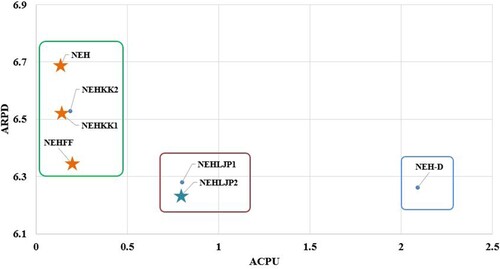
5.4. Efficiency evaluation of NEHLJP2

To confirm the computational efficiency of the NEHLJP2 heuristic, the ARPD, the average central processing unit time (ACPU) and the average relative percentage time (ARPT) are employed at the same time (Fernandez-viagas, Ruiz, and Framinan 2017). The ACPU and ARPT of heuristic p are defined as $ACP{U}_p=\frac{{\sum }_{\mathrm{\forall }j}CP{U}_{j,p}}{J}$, $ARP{T}_p={\sum }_{\mathrm{\forall }j}\frac{CP{U}_{j,p}-AC{T}_j}{AC{T}_j}/\phantom{{\sum }_{\mathrm{\forall }j}\frac{CP{U}_{j,p}-AC{T}_j}{AC{T}_j}J}J+1$, where $CP{U}_{j,p}$ is the computation time on instance j by heuristic p, $J$ is the total number of instances, $AC{T}_j=\frac{{\sum }_{\mathrm{\forall }p}CP{U}_{j,p}}{P}$, and P is the total number of heuristics considered. ACPU and ARPT are two main performance measures in terms of computational efficiency, although the solution quality is also to be considered as a key performance factor, which is represented by ARPD.

Each heuristic is run 10 times independently. As stated in Fernandez-viagas, Ruiz, and Framinan (2017), NEHKK2 and the heuristic NEHFF implemented with PR_D and TB_FF are deemed to be efficient, and they are taken as references in this article. The remaining reference heuristics in this article are also included in the efficiency evaluation.

Figures 5–10 illustrate the ARPD values versus ARPT and ACPU of each reference heuristic. Several clusters can be found in each figure, and it is shown that NEH, NEHKK1, NEHKK2 and NEHFF are located in the cluster with computational efficiency. The cluster of NEHLJP1 and NEHLJP2 shows excellent ARPD values at the nominal cost of ACPU or ARPT. The non-dominated heuristics are marked with stars in each figure. It can be seen that NEHLJP2 is a new dominating heuristic that outperforms the existing ones in terms of ARPD. This is the main contribution of this article, in developing a new priority and presenting a new heuristic, NEHLJP2.

Figure 5. Average relative percentage deviation (ARPD) versus average relative percentage time (ARPT) of heuristics on a logarithmic scale on the Taillard benchmark.

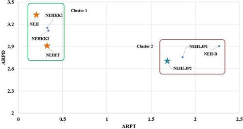
Figure 6. Average relative percentage deviation (ARPD) versus average central processing unit time (ACPU) of heuristics on a logarithmic scale on the Taillard benchmark.

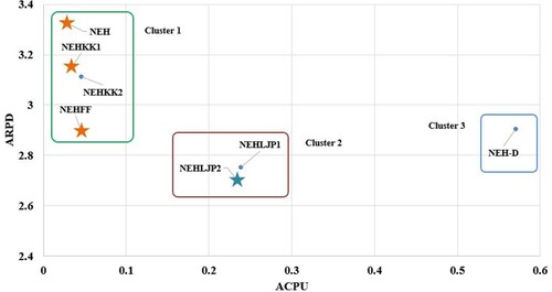
Figure 7. Average relative percentage deviation (ARPD) versus average relative percentage time (ARPT) of heuristics on a logarithmic scale on the VRF benchmark.

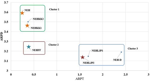
Figure 8. Average relative percentage deviation (ARPD) versus average central processing unit time (ACPU) of heuristics on a logarithmic scale on the VRF benchmark.

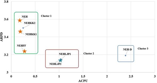
Figure 9. Average relative percentage deviation (ARPD) versus average relative percentage time (ARPT) of heuristics on a logarithmic scale on random instances.

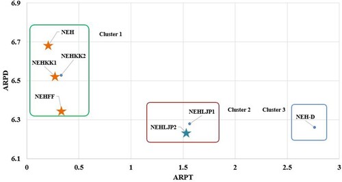
Figure 10. Average relative percentage deviation (ARPD) versus average central processing unit time (ACPU) of heuristics on a logarithmic scale on random instances.

5.5. Compatibility of NEHLJP2 with the IG algorithm

To further validate the new heuristic performance, all of the above NEH-based heuristics are used to generate an initial solution for the IG heuristic (Ruiz and Stützle 2007). The same hyperparameters from Liu, Jin, and Price (2018) are configured for the IG algorithm to conduct a fair performance comparison. Since the running time of the IG heuristic has an evident impact on the final results, different stopping criteria are defined. For example, the running time for the IG algorithm is set as n × m × 10 (milliseconds).

Figure 11 shows the results of NEH-IG, NEHKK1-IG, NEHKK2-IG, NEH-D-IG, NEHLJP1-IG and NEHLJP2-IG with the Taillard, VRF and random instances. It can be seen that NEHLJP2-IG can always obtain the best solution compared to the other heuristics.

Figure 11. Heuristic performance with the iterated greedy (IG) algorithm.

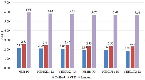
Table 11 show the results of the paired sample t-test of heuristics with the IG algorithm. By setting the running time of n × m × 10 milliseconds, NEHLJP2-IG shows significantly better performance than the heuristics. Again, the contribution of the new priority rule can be confirmed, in that it can be used for other metaheuristics with dominating performance.

Table 11. Paired sample t-test results of heuristics with the iterated greedy (IG) algorithm.

Pairs	Mean	SEM	CI lower	CI upper	T	Sig.
NEHLJP2_IG–NEHLJP1_IG	−0.03280	0.01457	−0.06138	−0.00422	−2.252	0.025
NEHLJP2_IG–NEHD_IG	−0.03551	0.01423	−0.06342	−0.00760	−2.496	0.013
NEHLJP2_IG–NEHKK2_IG	−0.16969	0.01443	−0.19800	−0.14138	−11.759	0.000
NEHLJP2_IG–NEHKK1_IG	−0.18156	0.01471	−0.21041	−0.15271	−12.346	0.000
NEHLJP2_IG–NEH_IG	−0.28178	0.01532	−0.31184	−0.25171	−18.389	0.000

6. Conclusions

In this article, a new perspective is developed to construct a new job priority rule, and the PFSP is studied. With the new perspective, the self-attention mechanism is introduced into production scheduling for the first time. The job similarities are calculated with the dot-product of job processing time matrices and taken as job weights to achieve job differentiation and ordering. Based on the new perspective, one new priority rule, namely PR_SAT, is proposed for makespan minimization, and by combining the TB_LJP1 tie-breaking rule, a heuristic, NEHLJP2, is presented.

A systematic performance evaluation of the new priority rule and NEHLJP2 heuristic is conducted with Taillard, VRF and 640 randomly generated instances. The experimental results confirm that the new priority rule with O(n²m) complexity achieves the best performance compared with existing rules in terms of makespan. The heuristic NEHLJP2 shows the best and a robust performance with different benchmarks. It obtains the best performance with the IG heuristic as well.

In the future, the new perspective can be further investigated and developed for the PFSP variants, such as no-idle or no-wait PFSPs. Different optimization criteria can be studied with the new perspective by adjusting the scaling factor. The new priority rule or NEHLJP2 can also be used for job dispatching or to provide an initial solution for other composite algorithms.

Acknowledgements

The authors are sincerely thankful to the editors and the anonymous referees who provided valuable and constructive comments to improve the technical content and presentation of the article.

Disclosure statement

No potential conflict of interest was reported by the authors.

Data availability statement

The data sets generated in the current study are available in the Mendeley Data repository, doi: 10.17632/gx8657vph2.1.

Additional information

Funding

This research is supported by the Natural Science Foundation of Shandong Province [grant number ZR2021QG001], the Youth Foundation of Social Science and Humanity, China Ministry of Education [grant number 21YJC630084], and the National Natural Science Foundation of China [grant number 72101136].

References

- Alfieri, A. 2009. “Workload Simulation and Optimisation in Multi-criteria Hybrid Flowshop Scheduling: A Case Study.” International Journal of Production Research 47 (18): 5129–5145. doi:10.1080/00207540802010823
- Baskar, A., and M. Anthony Xavior. 2021. “New Idle Time-Based Tie-Breaking Rules in Heuristics for the Permutation Flowshop Scheduling Problems.” Computers and Operations Research 133 (April): 105348. doi:10.1016/j.cor.2021.105348
- Benavides, Alexander J, Alexander J Benavides, Universidad Católica, and San Pablo. 2018. “A New Tiebreaker in the NEH Heuristic for the Permutation Flow Shop Scheduling Problem.” EasyChair Preprint 440. doi:10.29007/ch1l.
- Bengio, Yoshua, Andrea Lodi, and Antoine Prouvost. 2018. “Machine Learning for Combinatorial Optimization: A Methodological Tour d’Horizon,” 1–34. http://arxiv.org/abs/1811.06128.
- Choi, S.-W., Y.-D. Kim, and G.-C. Lee. 2005. “Minimizing Total Tardiness of Orders with Reentrant Lots in a Hybrid Flowshop.” International Journal of Production Research 43 (11): 2149–2167. doi:10.1080/00207540500050071
- Dong, X., H. Huang, and P. Chen. 2008. “An Improved NEH-Based Heuristic for the Permutation Flowshop Problem.” Computers & Operations Research 35 (12): 3962–3968. doi:10.1016/j.cor.2007.05.005
- Erseven, Göksu, Gizem Akgün, Aslıhan Karakaş, Gözde Yarıkcan, Özgün Yücel, and Adalet Öner. 2019. “An Application of Permutation Flowshop Scheduling Problem in Quality Control Processes.” Proceedings of the International Symposium for Production Research 2018.
- Fernandez-Viagas, V., and J. M. Framinan. 2014. “On Insertion Tie-Breaking Rules in Heuristics for the Permutation Flowshop Scheduling Problem.” Computers & Operations Research 45: 60–67. doi:10.1016/j.cor.2013.12.012
- Fernandez-viagas, Victor, Rubén Ruiz, and Jose M. Framinan. 2017. “A New Vision of Approximate Methods for the Permutation Flowshop to Minimise Makespan: State-of-the-Art and Computational Evaluation.” European Journal of Operational Research 257 (3): 707–721. doi:10.1016/j.ejor.2016.09.055
- Framinan, J. M., R. Leisten, and C. Rajendran. 2003. “Different Initial Sequences for the Heuristic of Nawaz, Enscore and Ham to Minimize Makespan, Idletime or Flowtime in the Static Permutation Flowshop Sequencing Problem.” International Journal of Production Research 41 (1): 121–148. doi:10.1080/00207540210161650
- Framinan, Jose M, Rainer Leisten, and Rafael Ruiz-Usano. 2005. “Comparison of Heuristics for Flowtime Minimisation in Permutation Flowshops.” Computers and Operations Research 32 (5): 1237–1254. doi:10.1016/j.cor.2003.11.002
- Gao, Jian, Rong Chen, and Wu Deng. 2013. “An Efficient Tabu Search Algorithm for the Distributed Permutation Flowshop Scheduling Problem.” International Journal of Production Research 51 (3): 641–651. doi:10.1080/00207543.2011.644819
- Jayamohan, M. S., and Chandrasekharan Rajendran. 2004. “Development and Analysis of Cost-Based Dispatching Rules for Job Shop Scheduling.” European Journal of Operational Research 157 (2): 307–321. doi:10.1016/S0377-2217(03)00204-2
- Kalczynski, P. J., and J. Kamburowski. 2008. “An Improved NEH Heuristic to Minimize Makespan in Permutation Flow Shops.” Computers & Operations Research 35 (9): 3001–3008. doi:10.1016/j.cor.2007.01.020
- Kalczynski, P. J., and J. Kamburowski. 2009. “An Empirical Analysis of the Optimality Rate of Flow Shop Heuristics.” European Journal of Operational Research 198 (1): 93–101. doi:10.1016/j.ejor.2008.08.021
- Kianfar, K., S. M. T. Fatemi Ghomi, and B. Karimi. 2009. “New Dispatching Rules to Minimize Rejection and Tardiness Costs in a Dynamic Flexible Flow Shop.” The International Journal of Advanced Manufacturing Technology 45 (7–8): 759–771. doi:10.1007/s00170-009-2015-x
- Kool, Wouter, Herke van Hoof, and Max Welling. 2018. “Attention Solves Your TSP, Approximately.” http://arxiv.org/abs/1803.08475.
- Koulamas, Christos, and S. S. Panwalkar. 2018. “New Index Priority Rules for No-Wait Flow Shops.” Computers and Industrial Engineering 115 (November 2017): 647–652. doi:10.1016/j.cie.2017.12.015
- Liu, Weibo, Yan Jin, and Mark Price. 2016. “A New Nawaz–Enscore–Ham-Based Heuristic for Permutation Flow-Shop Problems with Bicriteria of Makespan and Machine Idle Time.” Engineering Optimization 48 (10): 1808–1822. doi:10.1080/0305215X.2016.1141202
- Liu, Weibo, Yan Jin, and Mark Price. 2017a. “A New Improved NEH Heuristic for Permutation Flowshop Scheduling Problems.” International Journal of Production Economics 193 (June 2016): 21–30. doi:10.1016/j.ijpe.2017.06.026
- Liu, Weibo, Yan Jin, and Mark Price. 2017b. “New Scheduling Algorithms and Digital Tool for Dynamic Permutation Flowshop with Newly Arrived Order.” International Journal of Production Research 55 (11): 3234–3248. doi:10.1080/00207543.2017.1285077
- Liu, Weibo, Yan Jin, and Mark Price. 2018. “New Meta-heuristic for Dynamic Scheduling in Permutation Flowshop with New Order Arrival.” The International Journal of Advanced Manufacturing Technology 98: 1817–1830. doi:10.1007/s00170-018-2171-y
- Nagano, M. S., and J. V. Moccellin. 2002. “A High Quality Solution Constructive Heuristic for Flow Shop Sequencing.” Journal of the Operational Research Society 53 (12): 1374–1379. doi:10.1057/palgrave.jors.2601466
- Natarajan, K., K. M. Mohanasundaram, B. Shoban Babu, S. Suresh, K. Antony Arokia Durai Raj, and C. Rajendran. 2007. “Performance Evaluation of Priority Dispatching Rules in Multi-level Assembly Job Shops with Jobs Having Weights for Flowtime and Tardiness.” International Journal of Advanced Manufacturing Technology 31 (7–8): 751–761. doi:10.1007/s00170-005-0258-8
- Nawaz, M., E. E. Enscore, Jr., and I. Ham. 1983. “A Heuristic Algorithm for the m-Machine, n-Job Flow-Shop Sequencing Problem.” Omega 11 (1): 91–95. doi:10.1016/0305-0483(83)90088-9
- Ribas, Imma, Ramon Companys, and Xavier Tort-Martorell. 2010. “Comparing Three-Step Heuristics for the Permutation Flow Shop Problem.” Computers and Operations Research 37 (12): 2062–2070. doi:10.1016/j.cor.2010.02.006
- Rinnooy Kan, A. H. G. 1976. Machine Scheduling Problems: Classification, Complexity and Computations. The Hague, The Netherlands: Martinus Nijhoff. doi:10.1016/0377-2217(77)90029-7.
- Ruiz, R., and T. Stützle. 2007. “A Simple and Effective Iterated Greedy Algorithm for the Permutation Flowshop Scheduling Problem.” European Journal of Operational Research 177 (3): 2033–2049. doi:10.1016/j.ejor.2005.12.009
- Sauvey, Christophe, and Nathalie Sauer. 2020. “Two NEH Heuristic Improvements for Flowshop Scheduling Problem with Makespan Criterion.” Algorithms 13 (5): 1–14. doi:10.3390/a13050112
- Sha, D. Y., S. Y. Hsu, Z. H. Che, and C. H. Chen. 2006. “A Dispatching Rule for Photolithography Scheduling with an On-Line Rework Strategy.” Computers & Industrial Engineering 50 (3): 233–247. doi:10.1016/j.cie.2006.04.002
- Sharma, Meenakshi, Manisha Sharma, and Sameer Sharma. 2021. “An Improved Neh Heuristic to Minimize Makespan for Flow Shop Scheduling Problems.” Decision Science Letters 10 (3): 311–322. doi:10.5267/j.dsl.2021.2.006
- Swaminathan, Rajesh, Michele E. Pfund, John W. Fowler, Scott J. Mason, and Ahmet Keha. 2007. “Impact of Permutation Enforcement When Minimizing Total Weighted Tardiness in Dynamic Flowshops with Uncertain Processing Times.” Computers & Operations Research 34 (10): 3055–3068. doi:10.1016/j.cor.2005.11.014
- Taillard, E. 1993. “Benchmarks for Basic Scheduling Problems.” European Journal of Operational Research 64: 278–285. doi:10.1016/0377-2217(93)90182-M
- Tay, Joc Cing, and Nhu Binh Ho. 2008. “Evolving Dispatching Rules Using Genetic Programming for Solving Multi-objective Flexible Job-Shop Problems.” Computers and Industrial Engineering 54 (3): 453–473. doi:10.1016/j.cie.2007.08.008
- Vallada, E., R. Ruiz, and J. M. Framinan. 2015. “New Hard Benchmark for Flowshop Scheduling Problems Minimising Makespan.” European Journal of Operational Research 240 (3): 666–677. doi:10.1016/j.ejor.2014.07.033
- Vallada, Eva, Rubén Ruiz, and Gerardo Minella. 2008. “Minimising Total Tardiness in the m-Machine Flowshop Problem: A Review and Evaluation of Heuristics and Metaheuristics.” Computers & Operations Research 35 (4): 1350–1373. doi:10.1016/j.cor.2006.08.016
- Vaswani, Ashish, Noam Shazeer, Niki Parmar, Jakob Uszkoreit, Llion Jones, Aidan N. Gomez, Lukasz Kaiser, and Illia Polosukhin. 2017. “Attention Is All You Need,” no. Nips.
- Wang, Cheng, Shiji Song, Jatinder N.D. Gupta, and Cheng Wu. 2012. “A Three-Phase Algorithm for Flowshop Scheduling with Blocking to Minimize Makespan.” Computers and Operations Research 39 (11): 2880–2887. doi:10.1016/j.cor.2012.02.020
- Weng, Michael X., and Haiying Ren. 2006. “An Efficient Priority Rule for Scheduling Job Shops to Minimize Mean Tardiness.” IIE Transactions (Institute of Industrial Engineers) 38 (9): 789–795. doi:10.1080/07408170600710523
- Wu, Qinghua, Qingxuan Gao, Weibo Liu, and Shuai Cheng. 2021. “Improved NEH-Based Heuristic for the Blocking Flow-Shop Problem with Bicriteria of the Makespan and Machine Utilization.” Engineering Optimization. doi:10.1080/0305215X.2021.2010727
- Xiong, Hegen, Huali Fan, Guozhang Jiang, and Gongfa Li. 2017. “A Simulation-Based Study of Dispatching Rules in a Dynamic Job Shop Scheduling Problem with Batch Release and Extended Technical Precedence Constraints.” European Journal of Operational Research 257 (1): 13–24. doi:10.1016/j.ejor.2016.07.030