Landscape-enabled algorithmic design for the cell switch-off problem in 5G ultra-dense networks

Abstract

The rapid evolution of mobile communications, remarkably the fifth generation (5G) and research-stage sixth (6G), highlights the need for numerous heterogeneous base stations to meet high demands. However, the deployment of many base stations entails a high energy cost, which contradicts the concept of green networks promoted by next-generation networks. The Cell Switch-Off (CSO) problem addresses this by aiming to reduce energy consumption in ultra-dense networks without compromising service quality. This article explores the CSO problem from a multi-objective optimization perspective, focusing on how spatial network demand heterogeneity affects the multi-objective landscape of the problem. In addition to deep landscape understanding, it introduces a local search operator designed to exploit these landscape characteristics, improving the multi-objective efficiency of metaheuristics. The results indicate that increasing heterogeneity simplifies the exploration of the problem space, with the operator achieving closer approximations to the Pareto front, particularly in minimizing network power consumption.

Keywords:

• Exploratory landscape analysis
• multi-objective optimization
• metaheuristics
• energy efficiency
• 5G

List of abbreviations

5G	=	5th Generation of Mobile Communications
6G	=	6th Generation of Mobile Communications
BW	=	Bandwidth
CSO	=	Cell Switch-Off
EAF	=	Empirical Attainment Function
ELA	=	Exploratory Landscape Analysis
HetNet	=	Heterogeneous wireless cellular Network
HV	=	Hypervolume
ICT	=	Information and Communication Technologies
KPI	=	Key Performance Indicator
MIMO	=	Multiple-Input Multiple-Output
MOEA	=	Multi-Objective Evolutionary Algorithm
MOP	=	Multi-Objective Problem
NSGA-II	=	Non-Sorting Genetic Algorithm II
PC	=	Power Consumption
PLO	=	Pareto Local Optima
PPP	=	Poisson Point Process
QoS	=	Quality of Service
RPF	=	Reference Pareto Front
SA	=	Social Attractor
SBS	=	Small Base Station
SINR	=	Signal-to-Interference-plus-Noise Ratio
SNR	=	Signal-to-Noise Ratio
UDN	=	Ultra-Dense Network
UE	=	User Equipment

1. Introduction

Wireless communication technologies are under constant evolution motivated by use cases and application scenarios that require ever-increasing performance. From the first generation to the fifth (5G) (Agiwal, Roy, and Saxena 2016), these technologies have operated at higher frequency bands, larger bandwidths and higher data rates, providing users with enhanced quality of experience. Indeed, even before the first 5G networks were commercialized in 2019 and also coinciding with 5G standardization (Chen et al. 2023), industry, academia and standards organizations began to research the sixth generation (6G) of wireless communication systems (Salahdine, Han, and Zhang 2023; Tataria et al. 2021). Among the key enabling technologies already established for 5G (Andrews et al. 2014), the deployment of a large number of heterogeneous Small Base Stations (SBSs) to increase the spatial reuse of the spectrum was key to improving the network capacity to meet the expected system performance (Lopez-Perez et al. 2015). These are known as Ultra-Dense Networks (UDNs) (Gotsis, Stefanatos, and Alexiou 2016; Stoynov et al. 2023), and are still one of the key development trends for 6G (Salahdine, Han, and Zhang 2023; Wang et al. 2023).

In this context, both environmental sustainability and operational expenditures are two major issues in Information and Communication Technologies (ICT) (Freitag et al. 2021) in general, and in 5G/6G UDNs in particular (Mughees et al. 2021; Salahdine et al. 2021), as base stations account for 60% to 80% of the power consumption of the cellular network (Yao et al. 2019) and more than 1000 BSs/km${}^2$ are expected to be deployed (Lopez-Perez et al. 2015; Stoynov et al. 2023). This is especially critical in periods of low or no traffic demands, when most of the SBSs are not serving any user. In these scenarios, either switching off or entering SBSs into sleep mode has been proposed as a useful strategy to enhance energy efficiency (Kaur, Garg, and Kukreja 2023), which has even been included in the releases of standard bodies (3GPP 2014; Chen et al. 2023). The decision task of selecting which SBSs have to be deactivated has been approached in the literature from different perspectives such as clustering (Abubakar et al. 2022; Natarajan and Rebekka 2023a), game theory (Tinh et al. 2022) or, more recently, machine learning techniques (Natarajan and Rebekka 2023b; Ozturk et al. 2021; Tan et al. 2022). This decision problem has also been formulated as a combinatorial optimization problem, called Cell Switch Off (CSO) (Feng, Mao, and Jiang 2017), which is known to be NP-complete (González et al. 2016). All different flavours of the CSO problem, in either their static (Beitelmal et al. 2018) or dynamic (Luna et al. 2020) versions, must consider not only reducing the UDN energy consumption (trivially solved by deactivating all SBSs) but also any Key Performance Indicator (KPI) of the user Quality of Service (QoS). The CSO problem has been addressed with exact (Ahmed et al. 2021; Dolfi et al. 2017), heuristic (Femenias, Lassoued, and Riera-Palou 2020; Yang et al. 2023) and metaheuristic (Fourati et al. 2023) techniques, using single (Salem, El-Rabaie, and Shokair 2019; Venkateswararao and Swain 2022) versus multi-objective (González et al. 2016) approaches. This work falls into the latter research domain, where compromise solutions between energy consumption and network capacity are sought (Espinosa-Martínez et al. 2022; Galeano-Brajones et al. 2023; Luna et al. 2018), but aims to deepen the characterization of the multi-objective landscape of the CSO problem to obtain a fundamental understanding of its difficulty and design improved search strategies. Given the nature of CSO, it can be considered as a large-scale sparse multi-objective combinatorial optimization problem (Tian et al. 2020) because many SBSs can be deactivated when traffic demand is low.

This work has its roots in the seminal work on multi-objective combinatorial landscape analysis by Liefooghe et al. (2020), extending the study from multi-objective NK-landscapes to the CSO problem. It aims at gaining insights into how two major problem descriptors, namely the spatial distribution of both the network infrastructure (i.e. SBSs) and the traffic demand (i.e. user equipments, UEs), impact the problem landscape and, hence, the difficulty for multi-objective metaheuristics to address it properly. To the best of the present authors' knowledge, this is the first time a study of the CSO problem has been undertaken. Other features considered to characterize the CSO landscape are a set of several black-box local measures that have been estimated from a sample of solutions (Cosson et al. 2022) and computed over the smallest instances tackled in previous works that have more than 1000 decision variables (the LL scenarios in Galeano-Brajones et al. 2023). As this work pursues realistic settings, global measures have been avoided because they require a full enumeration of the solution space, such as the proportion of Pareto optimal solutions (Liefooghe et al. 2020), which is not computationally affordable in the context of this optimization problem.

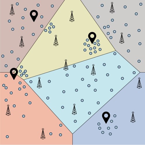
Experiments were conducted over a set of 800 instances with different levels of network densification (i.e. the number of SBSs and UEs per km${}^2$) and different degrees of non-uniformity in the SBSs and UE locations throughout the wireless network (i.e. heterogeneity in spatial traffic demand) (Mirahsan, Schoenen, and Yanikomeroglu 2015). The present authors have been able to provide empirical evidence indicating that, according to the exploratory landscape analysis, the closer SBSs and UEs are to each other (a higher non-uniform spatial distribution), the CSO problem becomes easier to solve. On the basis of these results, a novel local search operator that takes advantage of this severity in the heterogeneity of traffic demands has been devised. In order to show its effectiveness, a new set of instances has been generated in which the network is partitioned into several regions, each with different levels of traffic heterogeneity (see Figure 1). In summary, the main contributions of this work are as follows.

• This is the very first time in which a multi-objective exploratory landscape analysis on a realistic problem like CSO has been carried out. This has required a huge amount of computational effort as realistic instances have been considered for the landscape sampling to capture the inherent problem characteristics.

• A novel landscape-aware local search operator has been engineered to capitalize on previous findings.

• Extensive experiments have been carried out to show empirical evidence of the effectiveness of the newly developed operator.

Figure 1. A wireless network with several regions, each one having a different level of non-uniformity in the spatial distribution of the traffic demands. The grey point denotes an SBS that includes sectors and cells.

The rest of the paper is organized as follows. Section 2 outlines the background of this work, defining the CSO problem and the tools used for landscape characterization. Section 3 delves deeply into the analysis of the exploratory landscape analysis of the CSO problem. Then, Section 4 defines the landscape-aware local search operator proposed. Section 5 presents the findings on landscape explorability with respect to heterogeneity and the landscape-aware operator. Finally, Section 6 summarizes the conclusions reached and outlines some future research directions.

2. Background

2.1. The CSO problem

This section provides the reader with the background related to this work. First, the CSO problem is described, beginning with the modelling of the ultra-dense 5G network, the strategy for user and base station deployment, and the formulation of the problem objectives. Then, the characterization of multi-objective landscapes is outlined.

2.1.1. Network modelling

The foundation of network modelling is based on the one used in previous research (see Section 3 of Galeano-Brajones et al. 2023). For this reason, we have decided to move the complete modelling to Appendix 1 of this article, limiting ourselves to describing the modifications made in this section.

Regarding the UE–cell association, two modifications have been made to the modelling. First, in previous work, the association was based on the highest SINR (Signal-to-Interference-plus-Noise Ratio) received by the UE. Since interferences are largely mitigated and can be disregarded due to intelligent frequency reuse (Al-Falahy and Alani 2017; Mohan and Giridhar 2022), this article opts instead for the use of the SNR (Signal-to-Noise Ratio). Therefore, the SNR in UE k is defined as follows: (1) $\begin{array}{r}{\mathrm{SNR}}_k[\mathrm{dB}]=P_{\mathrm{rx},j,k}[\mathrm{dBm}]-P_n[\mathrm{dBm}],\end{array}$(1) where $P_{\mathrm{rx},j,k}$ represents the signal power received by UE k from cell j, and $P_n$ denotes the noise power (Equation A5).

Secondly, the allocation mechanism adapted in this work is based on the theoretical maximum capacity that can be offered to the UE, assuming that the cell has no associated UEs and can dedicate its entire bandwidth to the UE. This mechanism encourages the association of UEs with smaller cells and higher working frequencies, which in turn provide greater capacity while inducing lower consumption.

2.1.2. Deployment strategy

It is common to find Poisson Point Processes (PPPs) being used in the scientific literature for the deployment of BSs and/or UEs in mobile networks. This is because PPPs provide a simple mathematical model to represent the random and spatial distribution in deployments. Additionally, they are useful because the locations of both BSs and UEs in the real world can be quite random and scattered. The PPP model can be extended or modified to accommodate additional network features, such as UEs clustering or spatial correlations, providing a good balance between accuracy and complexity.

In this sense, Mirahsan, Schoenen, and Yanikomeroglu (2015) proposed overcoming the limitations of PPPs through a heterogeneous spatial model that allows statistical adjustments. The model tweaks two statistical parameters related to the distribution of UEs: the coefficient of variation of a distance measure between UEs, and the correlation coefficient between the locations of UEs and BSs. This model is suggested for Heterogeneous wireless cellular Networks (HetNets) to demonstrate the impact of heterogeneous and correlated traffic with BSs on network performance.

Based on this model, the deployment process used is described as follows.

1. Deployment of BSs and UEs. First, the deployment of BSs and UEs is carried out following a PPP.

2. Deployment of social attractors (SAs). Subsequently, SAs are deployed randomly in this scenario. These SAs represent real-world points of interest for UEs, such as central streets, shopping centres, etc.

3. Adjustment of the location of SAs. Each SA is moved towards its nearest BS in terms of received power, by a factor of $\alpha \in [0,1]$. Therefore, the new location of the ith SA is as follows: (2) $\begin{array}{r}S{A}_i^{\mathrm{new}}=\mathrm{\alpha B}{S}_{S{A}_i}+(1-\alpha )S{A}_i^{\mathrm{old}},\end{array}$(2) where $S{A}_i^{\mathrm{new}}$ is the new location of the SA, $S{A}_i^{\mathrm{old}}$ is the initial location, and $B{S}_{S{A}_i}$ is the BS from which SA receives the highest power.

4. Adjustment of the locations of the UEs. With the SAs relocated, each UE is moved towards its nearest SA in terms of Euclidean distance, by a factor β. Consequently, the new location of the ith UE is (3) $\begin{array}{r}U{E}_i^{\mathrm{new}}=\mathrm{\beta S}{A}_{U{E}_i}+(1-\beta )U{E}_i^{\mathrm{old}},\end{array}$(3) where $U{E}_i^{\mathrm{new}}$ is the new location of the UE, $U{E}_i^{\mathrm{old}}$ is the initial location and $S{A}_{U{E}_i}$ is the closest SA. This approach, of UEs moving towards SAs, can lead to some areas of the network becoming devoid of UEs. This implies that the distribution of UEs does not change; it simply contracts towards the SAs. To address this problem, the authors of Mirahsan, Schoenen, and Yanikomeroglu (2015) modified the value of β, shifting from a fixed value to modelling it as a random variable $\beta \sim \mathcal{N}({\mu }_{\beta },{\sigma }_{\beta })$, where ${\mu }_{\beta }$ is the mean of β and ${\sigma }_{\beta }$ is defined as ${\sigma }_{\beta }=(0.5-|{\mu }_{\beta }-0.5|)/3$ to minimize the probability that β falls outside $[0,1]$. Thus, instead of moving all UEs towards the SAs by a fixed value, the amount of movement is varied according to a normal distribution, which aids in maintaining a more uniform distribution of UEs across the scenario and preventing areas without UEs.

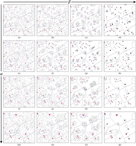
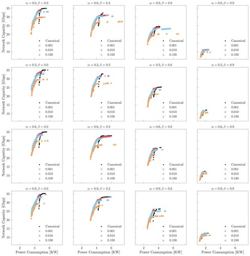
Consequently, by modifying the factors α and β, the spatial distribution of the UEs can be altered in this scenario. This distribution alteration is visible in Figure 2, which illustrates the deployments for combinations of α and β that arise from all combinations of values $[0.0,0.3,0.6,0.9]$. Moving to the right implies an increase in the value of β, while moving down indicates an increase in α. Furthermore, each combination of α and β entails limits on the maximum values of the two problem objectives, since a higher concentration of UEs near SBSs will concentrate allocations in a smaller number of cells, thereby resulting in lower consumption, since more cells can be switched off, and lower capacity such as bandwidth is shared among more UEs.

Figure 2. Deployments of UEs and SBSs for combinations of α and β resulting from combining the values 0.0, 0.3, 0.6 and 0.9 for each parameter. In the matrix, moving down the rows indicates an increase in α, while moving to the right in the columns implies an increase in β (Mirahsan, Schoenen, and Yanikomeroglu 2015).

2.1.3. Problem objectives

Let $\mathcal{B}$ be the set of SBSs deployed by a PPP and ${\mathcal{C}}_b$ the set of cells in SBS b, for every $b\in \mathcal{B}$. A CSO solution is represented as a bitstring s, where $s_c^b$ indicates whether the cell c in SBS b is active or not. The first objective, minimizing Power Consumption (PC), is achieved as follows: (4) $\begin{array}{r}min{f}_{\mathrm{PC}}(s)=\sum _{b\in \mathcal{B}}{P}_b\sum _{c\in {\mathcal{C}}_b}{s}_c^b,\end{array}$(4) where $P_b$ represents the power consumption of SBS b (as detailed in Equation A8). It is important to note that $P_b$ includes both the transmission power of each cell c within $C_b$ and the maintenance power.

Next, to calculate the total capacity of the system, the UEs initially associate themselves with the active cell, providing them with the highest theoretical capacity. Let $\mathcal{U}$ be the set of UEs, also deployed by a PPP, $\mathcal{C}$ the complete set of cells within $\mathcal{B}$, and $\mathcal{A}(s)\in {(0,1)}^{|\mathcal{U}|\times |\mathcal{C}|}$ the matrix where $a_{\mathrm{ij}}=1$ if $s_j=1$ and cell j serves the UE i with the highest theoretical capacity, and $a_{\mathrm{ij}}=0$, otherwise. The second objective, which is to maximize the total capacity (Cap) provided to all UEs, is calculated as follows: (5) $\begin{array}{rl}max{f}_{\mathrm{Cap}}(s)& =\sum _{c\in C}min(C_c^{\mathrm{cumulative}}(s),C_c^{max})\end{array}$(5) (6) $\begin{array}{rl}{C}_c^{\mathrm{cumulative}}(s)& =\sum _{i=1}^{\left|\mathcal{U}\right|}\sum _{j=1}^{\left|\mathcal{C}\right|}{s}_j\cdot a_{\mathrm{ij}}\cdot C_i^j,\end{array}$(6) where $C_c^{\mathrm{cumulative}}(s)$ is the cumulative capacity that cell $c\in C$ provides to the UEs in the scenario. $C_c^{max}$ represents the maximum capacity that cell c can offer, calculated assuming an SNR $=25$ dB. $C_i^j$ denotes the capacity that cell j provides to UE i (as detailed in Equation A6). The term $min(C_c^{\mathrm{cumulative}}(s),C_c^{max})$ ensures that capacities that exceed the maximum capacity threshold set in cells are not added to the capacity objective. It is crucial to note that the two objectives of the problem are conflicting: turning off cells leads to reduced network consumption but also affects the capacity provided to UEs. This conflict occurs because the switching off of cells increases the UE–cell distance (leading to higher propagation losses) and decreases the available bandwidth for serving the UEs.

It is also crucial to note the assumption that there is always a macrocell on in the scenario to prevent UEs from losing service. This macro cell is not included in the calculations of the objectives of the problem because the goal is to optimize the ultra-dense heterogeneous network. This provision ensures that, despite efforts to conserve energy by switching off certain cells, the fundamental service provision of the network (its capacity to connect UEs) is preserved, aligning with the core objective of balancing energy efficiency with service quality in ultra-dense network environments.

2.2. Multi-objective landscape characterization

This section briefly describes the multi-objective landscape features that are the basis of this work, which can be categorized into global and local features, as defined in Liefooghe et al. (2020), and how they are measured. On the one hand, global features require enumerating the entire search space to be computed. They include, for example, the proportion of Pareto optimal solutions, the distance between them, their connectedness, etc. Given the context of the present problem, set within a realistic scenario where the smallest instance of interest contains over 1000 binary decision variables, these characteristics become impractical. On the other hand, local features are computed from the neighbourhood of a sample of solutions and make the numerical effort affordable.

Before going into the details of the particular measures used, it is important to describe how sampling is performed. As defined in the previous section, a solution to the CSO problem is a binary string, and for such a representation, a neighbourhood structure has been used at a Hamming distance of one. Therefore, sampling is a walk over such an induced landscape, defined as an ordered sequence of solutions $(x_0,x_1,\dots ,x_l)$, such that $x_t$ is neighbour of $x_{t-1}$ (Weinberger 1990). Walks can be either random when neighbours are selected randomly at each step, or adaptive when an improved neighbour is required for the walk to continue. Random walks enable the computation of the first autocorrelation coefficient, which is a measure that characterizes the ruggedness of the landscape (the larger, the smoother) (Moser, Gheorghita, and Aleti 2017; Weinberger 1990). This autocorrelation measure does not make sense in adaptive walks, as the solutions are better at each step. Finally, while the length of a random walk, l, is defined in advance, for adaptive walks, this measure is the number of steps until the walk gets trapped in a local optimum.

3. Landscape analysis of the CSO problem

This section outlines the landscape features and descriptors of the CSO problem used in this study, as well as the experimental setup that includes the preliminary studies and the correlations obtained.

3.1. Landscape features

Before describing the experimental setup, it is crucial thoroughly to understand each of the landscape features used in this study and the descriptors of the CSO problem. Table 1 contains the nomenclature for each feature or descriptor, a brief description, and, where applicable, the reference to the work from which it was derived.

Table 1. Problem descriptors, multi-objective landscape features, and characteristics of the solutions considered in this article.

	Problem descriptors
α	Closeness factor of the SA to the nearest SBS	Equation (2(2) $\begin{array}{r}S{A}_i^{\mathrm{new}}=\mathrm{\alpha B}{S}_{S{A}_i}+(1-\alpha )S{A}_i^{\mathrm{old}},\end{array}$(2) )
β	Closeness factor of the UE to the nearest SA	Equation (3(3) $\begin{array}{r}U{E}_i^{\mathrm{new}}=\mathrm{\beta S}{A}_{U{E}_i}+(1-\beta )U{E}_i^{\mathrm{old}},\end{array}$(3) )
	Local landscape features related to the HV indicator
hv_avg	Average single solution's HV value	Liefooghe et al. (2020)
hv_r1	First autocorrelation coefficient of single solution's HV value (from random walks)	Liefooghe et al. (2013)
hvd_avg	Average single solution's HV difference value	Liefooghe et al. (2020)
hvd_r1	First autocorrelation coefficient of single solution's HV difference value (from random walks)	Liefooghe et al. (2013)
nhv_avg	Average neighbourhood's HV value	Liefooghe et al. (2020)
nhv_r1	First autocorrelation coefficient of neighbourhood's HV value (from random walks)	Liefooghe et al. (2020)
	Local landscape features related to the Pareto dominance
#inf_avg	Average proportion of neighbours dominated by the current solution	Liefooghe et al. (2020)
#inf_r1	First autocorrelation coefficient of the proportion of neighbours dominated by the current solution (from random walks)	Liefooghe et al. (2020)
#sup_avg	Average proportion of neighbours dominating the current solution	Liefooghe et al. (2020)
#sup_r1	First autocorrelation coefficient of the proportion of neighbours dominating the current solution (from random walks)	Liefooghe et al. (2020)
#inc_avg	Average proportion of neighbours incomparable with the current solution	Liefooghe et al. (2020)
#inc_r1	First autocorrelation coefficient of the proportion of neighbours incomparable with the current solution (from random walks)	Liefooghe et al. (2020)
	Features of the solutions
#micro_sbs_on_avg	Average proportion of active micro-SBS
#micro_sector_on_avg	Average proportion of active micro-sectors
#micro_cell_on_avg	Average proportion of active microcells
#pico_sbs_on_avg	Average proportion of active micro-SBS
#pico_sector_on_avg	Average proportion of active micro-sectors
#pico_cell_on_avg	Average proportion of active microcells
#femto_sbs_on_avg	Average proportion of active micro-SBS
#femto_sector_on_avg	Average proportion of active micro-sectors
#femto_cell_on_avg	Average proportion of active microcells
#micro_ue_avg	Average proportion of UEs allocated with microcells
#pico_ue_avg	Average proportion of UEs allocated with picocells
#femto_ue_avg	Average proportion of UEs allocated with femtocells
micro_dist_avg	Average distance from the nearest microcell to the UEs
pico_dist_avg	Average distance from the nearest picocell to the UEs
femto_dist_avg	Average distance from the nearest femtocell to the UEs
f_cor	Estimated correlation between the objective values (from random walks)	Liefooghe et al. (2020)
obj1_avg	Average single solution's value of the first objective	Equation (4(4) $\begin{array}{r}min{f}_{\mathrm{PC}}(s)=\sum _{b\in \mathcal{B}}{P}_b\sum _{c\in {\mathcal{C}}_b}{s}_c^b,\end{array}$(4) )
obj1_r1	First autocorrelation coefficient of the single solution's value of the first objective (from random walks)
obj2_avg	Average single solution's value of the second objective	Equation (5(5) $\begin{array}{rl}max{f}_{\mathrm{Cap}}(s)& =\sum _{c\in C}min(C_c^{\mathrm{cumulative}}(s),C_c^{max})\end{array}$(5) )
obj2_r1	First autocorrelation coefficient of the single solution's value of the second objective (from random walks)
walk_length	Average length of adaptive walks	Verel et al. (2013)

Regarding the problem descriptors, two proximity factors can be shown. As detailed in Section 2.1.2, the first is the proximity factor of each SA to the closest SBS, denoted as α, and the second is the proximity factor of each UE to its closest SA, denoted as β. These descriptors are fundamental for the subsequent discussion of the correlations and the design of the landscape-aware local search operator.

Following the problem descriptors in Table 1, we can show the local landscape features classified into three types: those related to the hypervolume indicator (HV) (Zitzler and Thiele 1999), Pareto dominance and the solutions. The first two types are based on the work of Liefooghe et al. (2020), while the last type is predominantly a contribution of this study. It is important to note that, as detailed in Section 2.2, obtaining the correlation between the objectives and the autocorrelation coefficients is not useful for adaptive walks. HV is a Pareto-compliant quality indicator widely used in the multi-objective community because it is able to gather information about the convergence and diversity of non-dominated solutions among the approximations to the Pareto front in one scalar value. It is computed by summing up the volume in the objective space enclosed by a given set of the non-dominated solutions. The higher the HV, the better.

Regarding the HV, three features are identified: hv_avg, hvd_avg and nhv_avg. The first feature provides information on the average HV of the solutions in the walk, the second gives the average HV difference between the solutions of the walk and those of each neighbourhood, and the last indicates the average HV of each neighbourhood. Moreover, from random walks, the first autocorrelation coefficients (called r1) for these three features (hv_r1, hvd_r1 and nhv_r1) can also be obtained. As explained in Section 2.2, the first autocorrelation coefficient of features related to HV provides information on the ruggedness of the landscape. In particular, a strong correlation with hv_r1 indicates that local improvements are easily achievable through neighbourhood exploration. This information is crucial for the local improvement strategy proposed in this article for the CSO problem.

Furthermore, features related to the dominance among the solutions of the walk and their neighbourhoods can be derived, in addition to those associated with HV. In this sense, the proportion of dominated neighbours (#inf_avg), dominating neighbours (#sup_avg) and incomparable neighbours (#inc_avg) are found. The first autocorrelation coefficients are also obtained for these features to observe trends in dominance throughout the random walks.

Among the other features of the solution, some define proportions (starting with #) and are identified by the type of cell (micro, pico or femto) and the type of support structure (SBS, sector or cell). In this context, some features define the average proportion of active structures for microcells (#micro_sbs_on_avg, #micro_sector_on_avg and #micro_cell_on_avg), picocells (#pico_sbs_on_avg, #pico_sector_on_avg and #pico_cell_on_avg) and femtocells (#femto_sbs_on_avg, #femto_sector_on_avg and #femto_cell_on_avg). An SBS and a sector are considered active if at least one of their cells is active. Furthermore, the average proportion of UEs allocated to each type of cell is defined as a descriptor (#micro_ue_avg, #pico_ue_avg and #femto_ue_avg). Furthermore, another defined descriptor is the average distance from each UE to the nearest cell of each type (micro_dist_avg, pico_dist_avg and femto_dist_avg). The features related to the objectives of the problem are also defined: first, there is an estimation of the correlation between the objective values obtained from random walks (f_cor); secondly, the average values of the objectives from the walk (obj1_avg and obj2_avg) are obtained along with their correlation coefficients (obj1_r1 and obj2_r1). Finally, from adaptive walks, the walk length (walk_length) can be obtained in order to know the number of steps needed to reach a Pareto Local Optimum (PLO).

3.2. Experimental setup

3.2.1. Preliminary studies

Given that the CSO problem is a real-world telecommunication challenge, the computational costs (both memory and computational time) are considerable. For this reason, before performing the walks, collecting landscape features and problem descriptors, as well as calculating correlations, preliminary studies were conducted to improve efficiency without losing landscape information on the problem.

As described in Appendix 1, nine types of scenario are defined with different densities of SBSs and UEs for the problem. Additionally, 50 different random seeds are used to generate 50 similar instances of the scenario, each consistent in terms of the densities of SBSs and UEs. Consequently, a total of 450 instances were dealt with. Therefore, before beginning the exploratory landscape analysis, consistency tests of the features across the different density scenarios were performed. This approach allowed working with the 50 seeds of the lower-density scenario (that is, the one requiring the smaller computational resources) to be focused on, so that the conclusions drawn could be extrapolated to the rest of the nine scenarios. Following this preliminary study, it was concluded that there were no significant differences in the correlations found across the nine scenarios. Hence, it was decided to focus on the lower-density scenario for exploratory landscape analysis in this work.

Then, another study was conducted to determine the maximum length of the random walks. To be consistent with previous works where the present authors used 100,000 evaluations as the stopping condition of the algorithms, it was decided to set the walk size to the same number. However, a significant time challenge was faced: exploring the entire neighbourhood at each step of the walk. As mentioned above, the present analysis focused on the lower-density instance, meaning fewer decision variables. However, considering the landscape analysis required to evaluate the entire neighbourhood at each step of the walk, roughly about 120 million evaluations per walk would have been needed to be performed, which is infeasible for a real-world problem. Consequently, it was decided to evaluate if, instead of exploring the entire neighbourhood, just a portion of it could be explored, which resulted in the authors' being able to limit their exploration to 5% of the neighbourhood without losing information on the correlations while achieving a significant gain in computational time. The selection of which neighbours to explore was carried out through a random sampling of the complete neighbourhood.

3.2.2. Correlations

In the analysis of landscape characteristics in multi-objective problems, understanding the interdependencies between different variables is crucial. For this purpose, the Kendall rank correlation coefficient (Hollander, Wolfe, and Chicken 2013), τ, which is a robust and non-parametric statistical measure, is used to quantify the association between two variables. The coefficient τ is calculated based on the number of concordant and discordant pairs in the dataset. A data pair is considered concordant if the observations in both variables maintain the same order; that is, if one observation is greater than another in one variable, it is also greater in the other. Conversely, a pair is deemed discordant when the order of observations in the two variables is opposite. The coefficient τ is calculated using the formula $\tau =\frac{N_c-N_d}{\sqrt{(N_0-N_1)(N_0-N_2)}},$where $N_c$ and $N_d$ represent the number of concordant and discordant pairs, respectively. Here, $N_0=n(n-1)/2$ is the total number of possible pairs in the dataset, with n being the number of observations. The terms $N_1=\sum t_i(t_i-1)/2$ and $N_2=\sum u_i(u_i-1)/2$ adjust the calculation of the ties within each of the variables, where $t_i$ and $u_i$ are the numbers of ties at the ith observation of each variable, respectively. A value of τ close to 1 indicates a strong positive correlation, while a value close to $-1$ implies a strong negative correlation. A value around zero implies no correlation. This coefficient is particularly useful in the present study as it does not assume a linear relationship between the variables and is resilient to the presence of outliers.

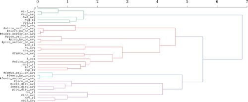
To display the correlations between different features and descriptors visually, correlation boards (see Figure 3) have been generated for samples from adaptive walks and random walks, which are interpreted similarly to a correlation matrix. Blue circles indicate a positive correlation, while red circles indicate a negative correlation (in darker or lighter gray, respectively, for B/W printed versions). The intensity of the colour and the size of the circle are proportional to the strength of the correlation. Additionally, to provide an alternative visualization of the relationship between features, dendrograms have been generated using Ward's hierarchical agglomerative clustering method (Murtagh and Legendre 2014). This method allows clusters of features to be separated based on their dissimilarity, offering another layer of information about the landscapes and the justification of the correlations visualized in the boards.

Figure 3. Correlation board for the features obtained through adaptive walks. Blue colour indicates a positive correlation, while red colour implies a negative correlation. Moreover, the intensity of the colour and the size of the circle are proportional to the strength of the correlation.

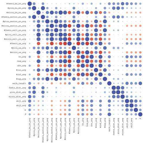
Taking into account the wide range of features to be analysed, this article focuses on three distinct subgroups: dominance, HV and solution features, with a special emphasis on the problem descriptors α and β. Additionally, the analysis of data collected through adaptive walks and random walks is conducted separately. This approach provides a comprehensive understanding of their respective behaviours within the solution space of the problem. Therefore, the correlations obtained through adaptive walks are represented on the correlation board in Figure 3, and in the dendrogram in Figure 4. Meanwhile, those obtained by random walks are shown in Figure 5, and the corresponding dendrogram in Figure 6.

Figure 4. Ward's dissimilarity measure among the features obtained through adaptive walks.

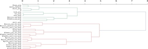
Figure 5. Correlation board for the features obtained through random walks.

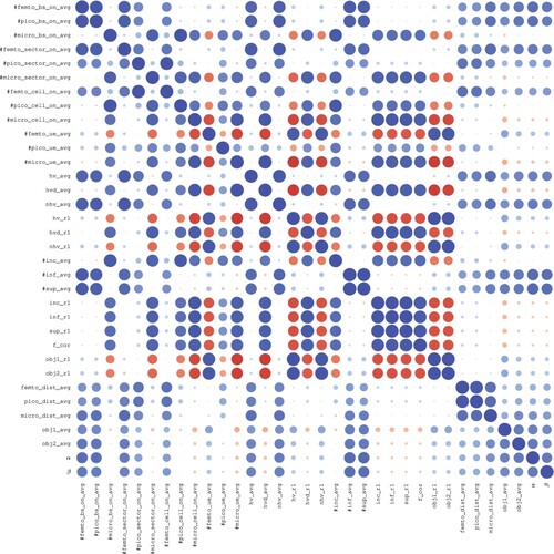
Figure 6. Ward's dissimilarity measure among the features obtained through random walks.

3.2.2.1 Dominance-related features for adaptive walks

From Figures 3 and 4, there is one main finding that can be drawn about the landscape and complexity of the problem, taking into account these features and the problem descriptors α and β. There is a strong correlation with walk_length, which suggests that, as long as SBSs and UEs are closer to each other (a higher level of clustering and, equivalently, a higher level of spatial heterogeneity in traffic demand), the landscape becomes easier to explore. Indeed, the number of steps of the adaptive walk increases, i.e. it is easier to find an improving solution. The positive correlation with obj1_avg, obj2_avg, hv_avg and nhv_avg corroborates this fact: the higher the values of α and β, the better the objectives of the problem, and thus the better the HV of the solutions and the neighbourhood. A clearer trend can be seen in Table 2, where the data collected over the different β values is aggregated for different landscape features. It can be seen that the proportion of non-dominated solutions (#inc_avg) decreases with β, whereas the proportion of worse/dominated (#inf_avg) and better/dominating #sup_avg solutions increases. That is, on the one hand, the landscape is more informative (fewer non-dominated solutions, thus reducing the existence of plateaus), and, on the other hand, the probability of moving to an improving neighbour increases. Further experimentation conducted in Section 5 will support this claim.

Table 2. Dominance-related landscape features aggregated over different values of β.

β	hv_avg	#inc_avg	#inf_avg	#sup_avg
0.0	0.5735	0.2010	0.5951	0.2017
0.3	0.5667	0.1864	0.6063	0.2051
0.6	0.5642	0.1460	0.6373	0.2147
0.9	0.6137	0.0718	0.6936	0.2328

3.2.2.2 HV-related features for adaptive walks

Apart from the correlations with hv_avg and nhv_avg discussed earlier, the negative correlation of α and β with hvd_avg suggests that a higher level of clustering implies greater variability in the HV of solutions compared to their neighbourhoods. This indicates that, as the spatial heterogeneity of traffic demands increases, the differences in HV between a solution and its surrounding solutions become less pronounced, reflecting a more uniform landscape. Therefore, higher values for α and β result in landscapes that are easier to explore.

3.2.2.3 Solution-related features for adaptive walks

The spatial heterogeneity generated by α and β also has effects on the features of the solution traversed by the adaptive walk. Specifically, greater heterogeneity tends to produce solutions with a higher proportion of UEs associated with femtocells (positive correlation with #femto_ue_avg) and lower with microcells (negative correlation with #micro_ue_avg). Given that hv_avg and nhv_avg correlate positively with #femto_ue_avg, it can be observed that the associations of solutions that improve the objectives of the problem and the HV are primarily made with femtocells. This hypothesis is reinforced by the positive correlation of #sup_avg and slightly negative correlation of #inf_avg with #femto_cell_on, indicating that cell activation favours neighbourhoods with a higher proportion of non-dominated solutions. Furthermore, the negative correlation of #femto_ue_avg with hvd_avg suggests that the difference in HV is smaller with a higher proportion of such associations. From this, it can be inferred that the ruggedness of the landscape is smoother in areas of high HV.

3.2.2.4 Dominance-related features for random walks

Regarding the dominance features from random walks, a clear conclusion can be drawn with α and β: greater clustering results in neighbourhoods with higher proportions of both dominated (strong positive correlation with #inf_avg) and non-dominated (strong positive correlation with #sup_avg) solutions compared to incomparable ones. This reinforces the hypothesis that a higher concentration of UEs towards SBSs makes the landscape easier to explore.

3.2.2.5 HV-related features for random walks

The strong positive correlations of the problem descriptors with hv_avg and nhv_avg indicate that the solutions tend to be of higher quality in random samplings, corroborating the hypothesis that the landscape becomes easier to explore.

3.2.2.6 Solution-related features for random walks

The correlations between the characteristics that define the proportion of active microcells and, to a lesser extent, picocells, with #inc_avg indicate that the highest proportion of incomparable solutions is found when many microcells are active and, therefore, when there is a higher hvd_avg. This suggests that the ruggedness of the landscape is greater, making it more difficult to explore. Additionally, #inf_avg and #sup_avg have a very positive correlation with cells operating at higher frequencies, particularly femtocells. Therefore, having a higher proportion of active femtocells, and to a lesser extent picocells, results in a higher proportion of both dominated and non-dominated solutions and a landscape easier to explore owing to the higher uniformity of the landscape, that is, less ruggedness. Consequently, it can be concluded that femtocells are key in guiding the search toward more promising areas of the landscape, while microcells present greater challenges. Regarding hv_r1, a negative correlation is observed with #micro_cell_on_avg, indicating that activating microcells leads to greater variability in HV throughout the walk. Furthermore, the strong positive correlation with #femto_ue_avg and negative with #micro_ue_avg suggest that favouring the use of femtocells tends to result in solutions with more similar HV values during the walk.

Finally, combining each analysis, two key conclusions can be drawn: a greater spatial heterogeneity in traffic demands results in a landscape that is easier to explore, and femtocells are of great importance for improving problem objectives and HV values. A previous paper (Galeano-Brajones et al. 2023) already elaborated on the line of this latter conclusion, in which the working hypothesis was that the activation of femtocells can improve the search process. This was demonstrated by devising problem-specific operators. Meanwhile, the first conclusion is further developed in this article through the design of a local search operator that leverages the information obtained with spatial traffic heterogeneity.

4. Landscape-aware local search

This section is devoted to describing the design of a local search operator that capitalizes on the knowledge acquired about the landscape characteristics detailed in the previous section. One of the key insights from the landscape analysis of the CSO problem is that greater spatial traffic heterogeneity makes local exploration of the search space easier. This is due to the proximity of UEs to SBSs, which makes higher-frequency cells (femtocells and, to a lesser extent, picocells) crucial for the optimization process. These types of cell have a low energy consumption and a high capacity, thus meeting the demands in small, highly-density areas. On the contrary, their size (i.e. the area they can serve) is small, thus UEs have to be close enough to establish a high-quality wireless link.

Algorithm 1 outlines the designed local search operator, which is based on performing a tailored adaptive walk (see Section 2.2) starting from a given solution chosen with a given rate, and that ends in a Pareto local optimum. The strategy of the operator is similar to that of a multi-objective hill climber. Still, the key aspect of the operator is the utilization of landscape information in the determination of how the neighbourhood of each solution is explored. In the standard case, the neighbourhood just consists of all solutions at a Hamming distance of one from the solution that is explored randomly (one randomly chosen neighbour at each time, moving only towards an improving one). The newly devised strategy uses the landscape information so that the neighbourhood is biased according to the value of the proximity factor β. This is achieved by the way the neighbourhood is explored, so that those cells located in areas where the spatial heterogeneity of the traffic demands is low (i.e. those in which β is known to be low and thus with a more difficult landscape) are visited first, to identify the improvement of neighbours in that area. Specifically, a Hamming neighbour would become part of the neighbourhood with a probability of $1-\beta$ (as detailed in lines 4–5 of Algorithm 2).

5. Results

This section presents a brief experimentation to validate the effectiveness of the local search operator that incorporates landscape information. First, the methodology is outlined, and then two experiments are conducted to, on the one hand, validate the hypothesis that increased spatial heterogeneity of traffic makes an easier landscape to explore and, on the other hand, to undertake a preliminary comparison between the newly devised aware operator and a standard multi-objective hill climber to show that the present authors' proposal can effectively profit from the landscape information.

5.1. Experimental methodology

NSGA-II (Deb et al. 2002) has been used as the baseline multi-objective solver in all the experiments. It has been configured to use a binary string representation with binary tournament selection, two-point crossover with a probability of 0.9, and bit flip mutation with a probability of 1/L, where L is the total number of cells in the scenario. Furthermore, 100,000 evaluations have been used as the stopping condition. This metaheuristic configuration is inherited from Galeano-Brajones et al. (2023).

NSGA-II has been hybridized by applying the local search operator right after the application of the crossover and mutation operators. The local search then starts from a given solution and continues until it converges to a Pareto local optimum, and at this point, it is inserted back into the population. The evaluations of the objective functions consumed during the search are also counted towards reaching the stopping condition for a fair comparison, which means that, if the local search is applied with higher probabilities, the number of NSGA-II iterations is reduced, thus limiting the evolutionary process. Regarding the probability of application of the operator, the experiments were conducted with values of 0.001, 0.010 and 0.100.

5.2. Analysis of the spatial heterogeneity impact on landscape explorability

For this exploratory analysis, the hybrid NSGA-II has been tested in 7200 different instances of the CSO problem, which is the result of performing an execution for each of the 50 different random seeds across the 9 density scenarios described in Appendix 1 and the 16 different heterogeneity factors devised in Figure 2 of Section 2.1.2. Considering the application of the three rates of the operator and the runs of the canonical metaheuristic, i.e. without the local search operator, a total of 28,000 runs have been carried out.

In Figure 7, the difference in the HV values between the runs with the application of the multi-objective hill climber and the canonical metaheuristic is displayed (the raw HV values can be found in Appendix 3). For this, the HV values have been averaged across all scenarios and seeds, in addition to the values of α, as β is the factor that shows more significant differences, as discussed in Section 3. This experiment aims to show that the HV difference tends to decrease with a higher value of β and, as a consequence, the exploration of the search space of the canonical NSGA-II with any intensification mechanism such as the multi-objective hill climber is able to reach much closer approximations to the Pareto fronts than those computed by the hybrid version of the algorithm. It can be concluded that the landscape can be easily explored when β is higher, i.e. when traffic demands (UEs) are more clustered around the SBSs (cells).

Figure 7. Average differences between the various application rates and the metaheuristic without local search.

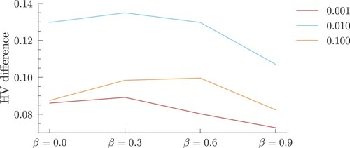
The fact that the difference slightly increases for medium heterogeneity values, especially for the application ratio of 0.010, may be because an increase in β for a higher α does not strictly indicate lower heterogeneity in some cases. In Figure 2 of Section 2.1.2, it is observed that in deployment (k), with a higher α, there is greater heterogeneity than in (g), although the factor is lower. This issue could be responsible for the values observed for medium heterogeneity.

To illustrate these differences visually, Figure 8 includes the attainment surfaces (Knowles 2005) for the HH scenario, the one with the highest density of UEs and SBSs. The Empirical Attainment Function (EAF) (Knowles 2005) facilitates a graphical examination of the approximated Pareto fronts. Specifically, the EAF visually represents the expected performance and its variability of the Pareto fronts approximated by the multi-objective algorithm across several iterations. To put it simply, within the context of multi-objective optimization, the 50%-attainment surface serves a role similar to the median in single-objective optimization scenarios. The rest of the scenarios can be consulted in Appendix 2. Therefore, in Figure 8 it can be observed that, as the values of α and β increase, the difference between the Pareto front approximations with and without the application of the search operator decreases to the point of being very similar fronts. This corroborates that greater heterogeneity eases the search, and the metaheuristic does not require local search operators to achieve similar results. On the contrary, lower heterogeneity creates a landscape more amenable to the local search operator, particularly for improving the power energy consumption objective of the network.

Figure 8. Approximations to the Pareto front for the different rates of application of the multi-objective hill climber in the HH scenario.

5.3. Comparative analysis of local search operators' performance

To verify the effectiveness of the landscape-aware operator and validate the findings drawn from the feature correlations in Section 3.2, the hybrid NSGA-II has been tested against 450 different instances. The spatial heterogeneity of traffic is divided into quadrants, with three of them exhibiting high heterogeneity ($\alpha =\beta =0.9$), and one with low heterogeneity ($\alpha =\beta =0.0$). Consequently, the landscape-aware operator will focus on improving the three quadrants with lower heterogeneity, which are inherently more challenging to explore, rather than concentrating efforts on the more navigable area of the landscape, i.e. the network area with higher heterogeneity. In contrast, the multi-objective hill climber does not differentiate between areas, performing searches regardless of heterogeneity (i.e. the neighbours to be explored are chosen in a randomly uniform manner).

Figure 9 displays the HV gain achieved by the landscape-aware operator compared to the multi-objective hill climber for three different application rates: 0.001, 0.01 and 0.1. The application rate of 0.1 consistently provides the highest gain across all nine density scenarios. The 0.001 rate shows improvements in the majority of scenarios, seven out of nine, but these are quite marginal. The 0.01 rate achieves the least gains, outperforming the operator in only three of the nine scenarios. Nevertheless, for all rates, there is a discernible trend in scenarios of higher density, and it is more advantageous to apply the landscape-aware operator.

Figure 9. HV gain achieved by the landscape-aware operator compared to the multi-objective hill climber for three different application rates.

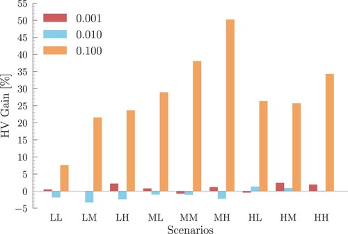
The results lead to the finding that landscape information, particularly regarding the spatial heterogeneity of network traffic, enables the enhancement of the outcomes of the metaheuristic. Conducting local searches targeted at more complex areas of the landscape allows the metaheuristic to achieve better approximations to the Pareto front, using the same stopping condition.

6. Conclusions and future work

After an in-depth analysis of the landscape of the CSO problem and after the examination of correlations between various features, this study has shown that an increase in the spatial heterogeneity of network traffic significantly smoothens the landscape, thus facilitating its exploration. To leverage this understanding, a novel search operator has been developed specifically to enhance multi-objective metaheuristics. This operator is designed to navigate the complexities of the landscape effectively, focusing on areas of the network characterized by lower heterogeneity. These regions, typically more challenging due to their uniformity, present unique opportunities for optimization that had previously been untapped. By strategically exploiting the information gleaned from the landscape analysis, the operator guides the search process towards more promising regions of the solution space. The empirical evidence presented confirms the efficacy of the operator, showcasing its ability to achieve better approximations to the Pareto front compared to traditional methods.

For future work, several directions are proposed that continue with the analysis of the problem landscape. First, an analysis of other problem descriptors, such as the association between UEs and cells, will be carried out. Secondly, the authors aim to continue the study of proposals for landscape-aware operators and genetic operators capable of operating with the information obtained from the landscape. Thirdly, a study will be conducted on the problem-specific operators proposed in previous works to examine how the shape of the landscape, influenced by heterogeneity, affects the effectiveness of the operators. Fourthly, owing to the sparse nature of the CSO problem, where optimal solutions often involve a minimal number of active cells, there is a compelling interest in further investigating the landscape for sparse solutions.

Acknowledgments

The authors thank the Supercomputing and Bioinformatics Centre of the Universidad de Málaga, for providing its services and the Picasso supercomputer facilities to perform the experiments (http://www.scbi.uma.es/).

Disclosure statement

No potential conflict of interest was reported by the author(s).

Data availability statement

The authors confirm that the data supporting the findings of this study are available within the article and its supplementary materials.

Additional information

Funding

This work has been partially funded by the Spanish Ministry of Science and Innovation [grants PID2020-112545RB-C54 and PID2020-112540RB-C41]; the European Union NextGenerationEU/PRTR [grants TED2021-131699B-I00 and TED2021-129938B-I00 (MCIN/AEI/10.13039/501100011033, FEDER)].

References

- 3GPP. 2014. Small Cell Enhancements for E-UTRA and E-UTRAN—Physical Layer Aspects. Technical report. 3rd Generation Partnership Project (3GPP). The 3GPP Organizational Partners. http://www.3gpp.org/ftp/Specs/html-info/36872.htm.
- Abubakar, Attai Ibrahim, Michael S. Mollel, Metin Ozturk, Sajjad Hussain, and Muhammad Ali Imran. 2022. “A Lightweight Cell Switching and Traffic Offloading Scheme for Energy Optimization in Ultra-Dense Heterogeneous Networks.” Physical Communication 52:101643. https://doi.org/10.1016/j.phycom.2022.101643.
- Agiwal, Mamta, Abhishek Roy, and Navrati Saxena. 2016. “Next Generation 5G Wireless Networks: A Comprehensive Survey.” IEEE Communications Surveys & Tutorials 18 (3): 1617–1655. https://doi.org/10.1109/COMST.2016.2532458.
- Ahmed, Faran, Muhammad Naeem, Waleed Ejaz, Muhammad Iqbal, Alagan Anpalagan, and Muhammad Haneef. 2021. “Energy Cooperation with Sleep Mechanism in Renewable Energy Assisted Cellular HetNets.” Wireless Personal Communications 116 (1): 105–124. https://doi.org/10.1007/s11277-020-07707-2.
- Al-Falahy, Naser, and Omar Y. K. Alani. 2017. “Network Capacity Optimisation in Millimetre Wave Band Using Fractional Frequency Reuse.” IEEE Access 6:10924–10932. https://doi.org/10.1109/Access.6287639.
- Andrews, Jeffrey G., Stefano Buzzi, Wan Choi, Stephen V. Hanly, Angel Lozano, Anthony C. K. Soong, and Jianzhong Charlie Zhang. 2014. “What Will 5G Be?.” IEEE Journal on Selected Areas in Communications 32 (6): 1065–1082. https://doi.org/10.1109/JSAC.2014.2328098.
- Beitelmal, Tamer, Sebastian S. Szyszkowicz, G. David González, and Halim Yanikomeroglu. 2018. “Sector and Site Switch-Off Regular Patterns for Energy Saving in Cellular Networks.” IEEE Transactions on Wireless Communications 17 (5): 2932–2945. https://doi.org/10.1109/TWC.7693.
- Chen, Wanshi, Xingqin Lin, Juho Lee, Antti Toskala, Shu Sun, Carla Fabiana Chiasserini, and Lingjia Liu. 2023. “5G-Advanced Toward 6G: Past, Present, and Future.” IEEE Journal on Selected Areas in Communications 41 (6): 1592–1619. https://doi.org/10.1109/JSAC.2023.3274037.
- Cosson, Raphaël, Bilel Derbel, Arnaud Liefooghe, Sébastien Verel, Hernan Aguirre, Qingfu Zhang, and Kiyoshi Tanaka. 2022. “Cost-vs-Accuracy of Sampling in Multi-Objective Combinatorial Exploratory Landscape Analysis.” In Proceedings of the Genetic and Evolutionary Computation Conference, Vol. 1, 493–501. New York: Association for Computing Machinery (ACM). https://dl.acm.org/doi/10 .1145/3512290.3528731.
- Deb, Kalyanmoy, Amrit Pratap, Sameer Agarwal, and T. A. M. T. Meyarivan. 2002. “A Fast and Elitist Multiobjective Genetic Algorithm: NSGA-II.” IEEE Transactions on Evolutionary Computation 6 (2): 182–197. https://doi.org/10.1109/4235.996017.
- Dolfi, Marco, Cicek Cavdar, Simone Morosi, Pierpaolo Piunti, Jens Zander, and Enrico Del Re. 2017. “On the Trade-Off Between Energy Saving and Number of Switchings in Green Cellular Networks.” Transactions on Emerging Telecommunications Technologies 28 (11): e3193. https://doi.org/10.1002/ett.v28.11.
- Espinosa-Martínez, Juan Jesús, Jesús Galeano-Brajones, Javier Carmona-Murillo, and Francisco Luna. 2022. “Binary Particle Swarm Optimization for Selective Cell Switch-Off in Ultra-Dense 5G Networks.” In Proceedings of the 13th International Conference on Swarm Intelligence (ANTS 2022), 275–283. Vol. 13491 of Lecture Notes in Computer Science. Cham, Switzerland: Springer. https://doi.org/10.1007/978-3-031-20176-9_23.
- Femenias, Guillem, Narjes Lassoued, and Felip Riera-Palou. 2020. “Access Point Switch ON/OFF Strategies for Green Cell-Free Massive MIMO Networking.” IEEE Access 8:21788–21803. https://doi.org/10.1109/Access.6287639.
- Feng, M., S. Mao, and T. Jiang. 2017. “Base Station ON-OFF Switching in 5G Wireless Networks: Approaches and Challenges.” IEEE Wireless Communications 24 (4): 46–54. https://doi.org/10.1109/MWC.2017.1600353.
- Fourati, Hasna, Rihab Maaloul, Lamia Fourati, and Mohamed Jmaiel. 2023. “An Efficient Energy-Saving Scheme Using Genetic Algorithm for 5G Heterogeneous Networks.” IEEE Systems Journal 17 (1): 589–600. https://doi.org/10.1109/JSYST.2022.3166228.
- Freitag, Charlotte, Mike Berners-Lee, Kelly Widdicks, Bran Knowles, Gordon S. Blair, and Adrian Friday. 2021. “The Real Climate and Transformative Impact of ICT: A Critique of Estimates, Trends, and Regulations.” Patterns 2 (9): 100340. https://doi.org/10.1016/j.patter.2021.100340.
- Galeano-Brajones, Jesús, Francisco Luna-Valero, Javier Carmona-Murillo, Pablo H. Zapata Cano, and Juan F. Valenzuela-Valdés. 2023. “Designing Problem-Specific Operators for Solving the Cell Switch-Off Problem in Ultra-Dense 5G Networks with Hybrid MOEAs.” Swarm and Evolutionary Computation 78:101290. https://doi.org/10.1016/j.swevo.2023.101290.
- González, David G., Jyri Hamalainen, Halim Yanikomeroglu, Mario Garcia-Lozano, and Gamini Senarath. 2016. “A Novel Multiobjective Cell Switch-Off Framework for Cellular Networks.” IEEE Access 4:7883–7898. https://doi.org/10.1109/ACCESS.2016.2625743.
- Gotsis, Antonis, Stelios Stefanatos, and Angeliki Alexiou. 2016. “UltraDense Networks: The New Wireless Frontier for Enabling 5G Access.” IEEE Vehicular Technology Magazine 11 (2): 71–78. https://doi.org/10.1109/MVT.2015.2464831.
- Hollander, Myles, Douglas A. Wolfe, and Eric Chicken. 2013. Nonparametric Statistical Methods. 3rd ed. Wiley Series in Probability and Statistics. Chichester, UK: Wiley.
- Kaur, Preetjot, Roopali Garg, and Vinay Kukreja. 2023. “Energy-Efficiency Schemes for Base Stations in 5G Heterogeneous Networks: A Systematic Literature Review.” Telecommunication Systems 84 (1): 115–151. https://doi.org/10.1007/s11235-023-01037-x.
- Knowles, Joshua 2005. “A Summary-Attainment-Surface Plotting Method for Visualizing the Performance of Stochastic Multiobjective Optimizers.” In Proceedings of the 5th International Conference on Intelligent Systems Design and Applications (ISDA'05), 552–557. Piscataway, NJ: IEEE.
- Liefooghe, Arnaud, Fabio Daolio, Sebastien Verel, Bilel Derbel, Hernan Aguirre, and Kiyoshi Tanaka. 2020. “Landscape-Aware Performance Prediction for Evolutionary Multiobjective Optimization.” IEEE Transactions on Evolutionary Computation 24 (6): 1063–1077. https://ieeexplore.ieee.org/document/8832171/.
- Liefooghe, Arnaud, Sébastien Verel, Hernán Aguirre, and Kiyoshi Tanaka. 2013. “What Makes an Instance Difficult for Black-Box 0–1 Evolutionary Multiobjective Optimizers?” In International Conference on Artificial Evolution (Evolution Artificielle), 3–15. Vol. 8752 of Lecture Notes in Computer Science. Cham, Switzerland: Springer. https://doi.org/10.1007/978-3-319-11683-9_1.
- Lopez-Perez, David, Ming Ding, Holger Claussen, and Amir H. Jafari. 2015. “Towards 1 Gbps/UE in Cellular Systems: Understanding Ultra-Dense Small Cell Deployments.” IEEE Communications Surveys & Tutorials 17 (4): 2078–2101. https://doi.org/10.1109/COMST.2015.2439636.
- Luna, F., R. M. Luque-Baena, J. Martínez, J. F. Valenzuela-Valdés, and P. Padilla. 2018. “Addressing the 5G Cell Switch-Off Problem with a Multi-Objective Cellular Genetic Algorithm.” In Proceedings of the IEEE 5G World Forum Conference (5GWF 2018), 422–426. https://doi.org/10.1109/5GWF.2018.8517066.
- Luna, Francisco, Pablo H. Zapata-Cano, Juan C. Gonzalez-Macias, and Juan F. Valenzuela-Valdés. 2020. “Approaching the Cell Switch-Off Problem in 5G Ultra-Dense Networks with Dynamic Multi-Objective Optimization.” Future Generation Computer Systems 110:876–891. https://doi.org/10.1016/j.future.2019.10.005.
- Mirahsan, Meisam, Rainer Schoenen, and Halim Yanikomeroglu. 2015. “HetHetNets: Heterogeneous Traffic Distribution in Heterogeneous Wireless Cellular Networks.” IEEE Journal on Selected Areas in Communications 33 (10): 2252–2265. https://doi.org/10.1109/JSAC.2015.2435391.
- Mohan, M. V. Abhay, and K. Giridhar. 2022. “Interference-Aware Accurate Signal Recovery in Sub-1 GHz UHF Band Reuse-1 Cellular OFDMA Downlinks.” IEEE Open Journal of the Communications Society 3:2087–2105. https://doi.org/10.1109/OJCOMS.2022.3219557.
- Moser, I., M. Gheorghita, and A. Aleti. 2017. “Identifying Features of Fitness Landscapes and Relating Them to Problem Difficulty.” Evolutionary Computation 25 (3): 407–437. https://doi.org/10.1162/evco_a_00177.
- Mughees, Amna, Mohammad Tahir, Muhammad Aman Sheikh, and Abdul Ahad. 2021. “Energy-Efficient Ultra-Dense 5G Networks: Recent Advances, Taxonomy and Future Research Directions.” IEEE Access9:147692–147716. https://doi.org/10.1109/ACCESS.2021.3123577.
- Murtagh, Fionn, and Pierre Legendre. 2014. “Ward's Hierarchical Agglomerative Clustering Method: Which Algorithms Implement Ward's Criterion?.” Journal of Classification 31 (3): 274–295. https://doi.org/10.1007/s00357-014-9161-z.
- Natarajan, Janani, and B. Rebekka. 2023a. “An Energy Efficient Dynamic Small Cell On/Off Switching with Enhanced k-Means Clustering Algorithm for 5G HetNets.” International Journal of Communication Networks and Distributed Systems 29 (2): 209–237. https://doi.org/10.1504/IJCNDS.2023.129230.
- Natarajan, Janani, and B. Rebekka. 2023b. “Machine Learning Based Small Cell ON/OFF for Energy Efficiency in 5G Heterogeneous Networks.” Wireless Personal Communications 130 (4): 2367–2383. https://doi.org/10.1007/s11277-023-10383-7.
- Ozturk, Metin, Attai Ibrahim Abubakar, Joao Pedro Battistella Nadas, Rao Naveed Bin Rais, Sajjad Hussain, and Muhammad Ali Imran. 2021. “Energy Optimization in Ultra-Dense Radio Access Networks Via Traffic-Aware Cell Switching.” IEEE Transactions on Green Communications and Networking 5 (2): 832–845. https://doi.org/10.1109/TGCN.2021.3056235.
- Piovesan, Nicola, Angel Fernandez Gambin, Marco Miozzo, Michele Rossi, and Paolo Dini. 2018. “Energy Sustainable Paradigms and Methods for Future Mobile Networks: A Survey.” Computer Communications 119:101–117. https://doi.org/10.1016/j.comcom.2018.01.005.
- Salahdine, Fatima, Tao Han, and Ning Zhang. 2023. “5G, 6G, and Beyond: Recent Advances and Future Challenges.” Annals of Telecommunications 78 (9–10): 525–549. https://doi.org/10.1007/s12243-022-00938-3.
- Salahdine, Fatima, Johnson Opadere, Qiang Liu, Tao Han, Ning Zhang, and Shaohua Wu. 2021. “A Survey on Sleep Mode Techniques for Ultra-Dense Networks in 5G and Beyond.” Computer Networks201:108567. https://doi.org/10.1016/j.comnet.2021.108567.
- Salem, A. A., S. El-Rabaie, and M. Shokair. 2019. “Energy Efficient Ultra-Dense Networks (UDNs) Based on Joint Optimisation Evolutionary Algorithm.” IET Communications 13 (1): 99–107. https://doi.org/10.1049/cmu2.v13.1.
- Son, J., S. Kim, and B. Shim. 2020. “Energy Efficient Ultra-Dense Network Using Long Short-Term Memory.” In Proceedings of the 2020 IEEE Wireless Communications and Networking Conference (WCNC), 1–6. Piscataway, NJ: IEEE. https://doi.org/10.1109/WCNC45663.2020.9120723.
- Stoynov, Viktor, Vladimir Poulkov, Zlatka Valkova-Jarvis, Georgi Iliev, and Pavlina Koleva. 2023. “Ultra-Dense Networks: Taxonomy and Key Performance Indicators.” Symmetry 15 (1): 2. https://doi.org/10.3390/sym15010002.
- Tan, Kang, Duncan Bremner, Julien Le Kernec, Yusuf Sambo, Lei Zhang, and Muhammad Ali Imran. 2022. “Graph Neural Network-Based Cell Switching for Energy Optimization in Ultra-Dense Heterogeneous Networks.” Scientific Reports 12 (1): 1–18. https://doi.org/10.1038/s41598-021-99269-x.
- Tataria, Harsh, Mansoor Shafi, Andreas F. Molisch, Mischa Dohler, Henrik Sjoland, and Fredrik Tufvesson. 2021. “6G Wireless Systems: Vision, Requirements, Challenges, Insights, and Opportunities.” Proceedings of the IEEE 109 (7): 1166–1199. https://doi.org/10.1109/JPROC.2021.3061701.
- Tian, Ye, Xingyi Zhang, Chao Wang, and Yaochu Jin. 2020. “An Evolutionary Algorithm for Large-Scale Sparse Multiobjective Optimization Problems.” IEEE Transactions on Evolutionary Computation 24 (2): 380–393. https://doi.org/10.1109/TEVC.4235.
- Tinh, Bui Thanh, Long D. Nguyen, Ha Hoang Kha, and Trung Q. Duong. 2022. “Practical Optimization and Game Theory for 6G Ultra-Dense Networks: Overview and Research Challenges.” IEEE Access10:13311–13328. https://doi.org/10.1109/ACCESS.2022.3146335.
- Venkateswararao, Kuna, and Pravati Swain. 2022. “Binary-PSO-Based Energy-Efficient Small Cell Deployment in 5G Ultra-Dense Network.” The Journal of Supercomputing 78 (1): 1071–1092. https://doi.org/10.1007/s11227-021-03910-5.
- Verel, Sébastien, Arnaud Liefooghe, Laetitia Jourdan, and Clarisse Dhaenens. 2013. “On the Structure of Multiobjective Combinatorial Search Space: MNK-Landscapes with Correlated Objectives.” European Journal of Operational Research 227 (2): 331–342. https://doi.org/10.1016/j.ejor.2012.12.019.
- Vucetic, Branka, and Jinhong Yuan. 2005. Performance Limits of Multiple-Input Multiple-Output Wireless Communication Systems, Chap. 1, 1–47. Chichester, UK: Wiley. https://doi.org/10.1002/047001413X.ch1.
- Wang, Cheng Xiang, Xiaohu You, Xiqi Gao, Xiuming Zhu, Zixin Li, Chuan Zhang, Haiming Wang, et al. 2023. “On the Road to 6G: Visions, Requirements, Key Technologies, and Testbeds.” IEEE Communications Surveys and Tutorials 25 (2): 905–974. https://doi.org/10.1109/COMST.2023.3249835.
- Weinberger, E. 1990. “Correlated and Uncorrelated Fitness Landscapes and How to Tell the Difference.” Biological Cybernetics 63 (5): 325–336. http://link.springer.com/10 .1007/BF00202749.
- Yang, Yi, Zhixin Liu, Heng Zhu, Xinping Guan, and Kit Yan Chan. 2023. “Energy Minimization by Dynamic Base Station Switching in Heterogeneous Cellular Network.” Wireless Networks 29 (2): 669–684. https://doi.org/10.1007/s11276-022-03167-7.
- Yao, Miao, Munawwar M. Sohul, Xiaofu Ma, Vuk Marojevic, and Jeffrey H. Reed. 2019. “Sustainable Green Networking: Exploiting Degrees of Freedom Towards Energy-Efficient 5G Systems.” Wireless Networks 25 (3): 951–960. https://doi.org/10.1007/s11276-017-1626-7.
- Zitzler, Eckart, and Lothar Thiele. 1999. “Multiobjective Evolutionary Algorithms: A Comparative Case Study and the Strength Pareto Approach.” IEEE Transactions on Evolutionary Computation 3 (4): 257–271. https://doi.org/10.1109/4235.797969.