Eddy-covariance flux measurements in an Italian deciduous forest using PTR-ToF-MS, PTR-QMS and FIS

ABSTRACT

A field campaign in a deciduous forest in Ispra, Italy, was performed by the Joint Research Centre, Ispra, Italy, together with University of Innsbruck, Austria, in 2013, using PTR-ToF-MS (proton transfer reaction – time-of-flight – mass spectrometry), PTR-QMS (proton transfer reaction – quadrupole mass spectrometry), FIS (fast isoprene sensor) and other instrumentations. The main purpose of the campaign was to measure volatile organic carbon (VOC). One of the outcomes of this investigation was the comparison between the three VOC measurement techniques, focusing on the VOC-flux values that could be measured, VOC-volume-mixing-ratio (VOC-VMR) values that could be measured, the number of VOCs identified/measured, and finally if any oxidation products from the primary emitted VOC could be identified/measured. To the best of our knowledge, it is the first time that these three techniques have been used simultaneously during a campaign in a forest, and the comparison of the three techniques is presented in details (PTR-ToF-MS, PTR-QMS and FIS). It was concluded that the isoprene data generated by the three instruments were in good agreement. With PTR-ToF-MS, the following main results were achieved during the summer campaign 2013: The VMR of isoprene was measured up to 16 ppb; large fluxes of isoprene with values up to 53 nmol m⁻² s⁻¹ by PTR-ToF-MS; mean diurnal (24 h) averages of VMR of isoprene of (1.07 ± 0.53) ppb and mean diurnal (24 h) flux of isoprene of (5.20 ± 2.42) nmol m⁻² s⁻¹. For the isoprene oxidation products methyl-vinyl-ketone/methacrolein (MVK/MACR), VMRs of (0.42 ± 0.22) ppb were measured as a mean diurnal (24 h) average. Mean diurnal (24 h) flux of MVK/MACR were measured to be (0.06 ± 0.04) nmol m⁻² s⁻¹; for the monoterpenes, the VMR was measured to be (0.10 ± 0.09) ppb mean diurnal (24 h) and mean diurnal (24 h) flux of monoterpenes to be (0.08 ± 0.05) nmol m⁻² s⁻¹. Detailed descriptions of the fluxes/VMRs of other VOCs, acetone/methanol/acetaldehyde, are also presented. The results obtained here have also been compared to several other similar studies and campaigns.

KEYWORDS:

• Flux
• volume mixing ratio VMR
• PTR-ToF-MS
• PTR-QMS
• FIS
• isoprene
• MVK/MACR
• terpenes

1. Introduction

Every year large amounts of volatile organic compounds (VOCs) are emitted into the atmosphere from natural and anthropogenic sources. It has been estimated that globally about 1150 Tg C yr⁻¹ of biogenic VOCs are emitted into the atmosphere, about 10 times greater than emissions of VOCs due to human activities [1,2]. Isoprene gives the largest contribution to biogenic VOC emissions; based on the MEGAN model, Sindelarova et al. [3] estimate that it accounts for 69% of the total, followed by the sum of monoterpenes which account for 11%. Uncertainties of biogenic VOC emissions are generally large; in the case of isoprene, they have been estimated to be around a factor of 2 [3].

Two important impacts of these large amounts of emitted biogenic VOCs are on the production of ozone and the formation of secondary organic aerosols in the atmosphere, both of which influence air quality, because ozone and aerosols are known to be harmful to human health [4–9]. In addition, organic aerosols also affect our climate, by scattering and absorption of solar radiation, or indirectly by acting as condensation nuclei for cloud droplets [10]. Tropospheric ozone is also known to be a strong greenhouse gas [11].

Tropospheric ozone VMR s have increased significantly during the last 100 years [12], mainly because of human activities, giving rise to emissions of large amounts of NOx and hydrocarbons to the troposphere. High-ozone concentrations at the surface are damaging to vegetation and reducing crop yields [13,14]. It is therefore important to investigate and understand the emissions and the fates of VOCs in the atmosphere as well as the formation and impact of ozone.

In this paper, we present an investigation of the emissions and fate of VOCs: A field campaign in a deciduous forest in Ispra, Italy, was performed by Joint Research Centre (JRC) in Ispra, Italy, together with University of Innsbruck, Austria, in 2013, using PTR-ToF-MS (proton transfer reaction – time-of-flight – mass spectrometry), PTR-QMS (proton transfer reaction – quadrupole mass spectrometry), FIS (fast isoprene sensor), and several other instrumentations. Additional information about the forest, tower, the nearby EMEP/GAW measuring station (within 500 m distance from the campaign site) and the ancillary instrumentations can be found in Ref. [15].

There have been several studies of VOC VMRs, emissions and fluxes from forests and other terrestrial areas (see e.g. [16–24]), but to the best of our knowledge this is the first investigation using all three VOC flux techniques (PTR-ToF-MS, PTR-QMS and FIS) simultaneously. We find that this type of comparison of different techniques is useful for obtaining realistic estimates of the error bars on flux measurements.

In this investigation we measured volume mixing ratios (VMRs) and fluxes of VOC masses in the mass range from 10 to 315 in a forest, which included biogenic VOCs: e.g. isoprene, monoterpenes, anthropogenic VOCs: e.g. benzene, toluene, xylenes and finally some atmospheric VOC oxidations products: e.g. MVK (methyl vinyl ketone), MACR (methacrolein), aldehydes, ketones, etc. One of the main aims of this investigation was the comparison of the three techniques: focusing on the VOC-flux/VMR values that could be measured, the number of VOCs identified/measured and finally if any oxidation products from the primary emitted VOC could be identified/measured. Another aim was the finding of the flux of isoprene and other VOCs and the comparison of these results with other studies. Finally, a discussion of the findings of the fluxes of oxygenated VOCs is presented.

2. Experimental

2.1 Field site description and meteorology

2.1.1 Field site description

The field measurement site was a deciduous forest at JRC-Ispra, in the North of Italy, mainly using the instruments PTR-ToF-MS, PTR-QMS and FIS. See Ref. [15] for more details about the forest, the flux tower station, and the nearby EMEP/GAW measuring station.

The forest flux station ‘IT-Isp’ is situated in a deciduous forest inside the JRC-Ispra site, in the North of Italy (location and altitude: 45.8127 N, 8.6340 E, and 209 m above sea level). The forest consists mostly of deciduous trees (Quercus robur L. (80%), Alnus glutinosa L. (10%), Populus alba L. (5%) and Carpinus betulus L. (3%)) with an average leaf area index of 4.2 m² m⁻². The height of the canopy was 26 m. The tower consists of a self-standing 36 m high structure with two platforms at 18 m and 36 m.

The instruments were placed in a 6 m × 3 m container with air conditioning, approximately 15 kW electrical power, local TCP/IP network to tower top with gateway to JRC-Ispra network, data acquisition PCs and Campbell data loggers (see Appendix 1 formore details in Suppl. info.). The flux tower station operated from mid-2012 until the end of 2015.

2.1.2 Meteorology

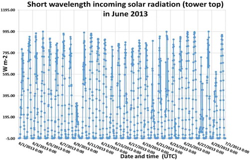
Meteorological observations were made for the whole month of June 2013 at the tower top where the intensive campaign took place (see Appendix 1 for more details): Measurements of temperature, relative humidity, wind speed and solar radiation (precipitation data were also measured at the campaign site and in June 2013 significant precipitation was observed only on the 2nd, 9th and 23rd of June 2013). In addition to these observations, meteorological data for the whole year of 2013 were also obtained directly at a nearby EMEP/GAW measuring station (less than 500 m from the campaign site) using the weather transmitter (T, P, RH) and a pyranometer (solar radiation) at 10 m and 1.5 m (2.5 m at the provisional site) above the ground, respectively (see Appendix 2 for these meteorological data Suppl. info.). Appendix 2 shows monthly values of these meteorological variables for 2013 as compared to the 1990–1999 average used as a reference period. June (when the intensive campaign took place) and July 2013 were exceptionally sunny and warm compared to the reference period, and January 2013 and February 2013 were particularly dry, while December 2013 was much rainier than usual compared to the reference period.

2.2 Apparatus and sampling air-tube

2.2.1 Apparatus

The analytical techniques applied here for VOCs were two types of PTR-MS (PTR-ToF-MS and PTR-QMS), and one type of FIS. The PTR-MS technique for online detection of VOCs developed by Lindinger et al. at the University of Innsbruck, Austria, has been thoroughly described and reviewed elsewhere [25,26].

More details of the instrumentation and the use of PTR-ToF-MS and PTR-QMS for VMR and flux measurements can be found elsewhere (e.g. [19,27–29].

2.2.2 PTR-QMS

As with the PTR-ToF-MS, the basis of the PTR-QMS is using H₃O⁺ for ionising VOCs so that they can be measured by mass spectrometry. For PTR-QMS, a hollow cathode (HC) discharge and a source drift region (SD) act as an ion source producing H₃O⁺ ions from pure water vapour. These ions are injected into a drift tube, which is continuously flushed with the air to be analysed at a pressure of approximately 2 mbar. The H₃O⁺ ions undergo non-reactive collisions with any of the common components in air (N₂, O₂, Ar, CO₂, etc.). Most VOCs have proton affinities (PAs) higher than that of water (PA(H₂O) = 7.22 eV), and in these cases a collision with the H₃O⁺ ion will result in the PTR for ionising the VOCs, and can thereafter be measured by mass spectrometry. The drift tube in the present investigation was operated at 587 V drift voltage and about 2.22 mbar drift tube pressure with the drift tube not heated, but drift tube measured to be 35 °C. E/N for PTR-QMS calculated to be 117 Td (references for this chapter about ‘PTR-QMS’, see e.g. Refs. [27,30,31].).

More details about the operational of PTR-QMS/PTR-MS can be found in Ref. [27,30–32].

2.2.3 PTR-ToF-MS

The recently developed ‘time-of-flight’ technique PTR-ToF-MS can measure 10 Hz time series of full mass spectra (mass range: 10–350) with a mass accuracy sufficient to separate most VOC of interest (e.g. by determining chemical formulas precisely and can thereby separate oxygen containing VOCs from pure hydrocarbons even if they have same masses). The PTR-ToF-MS drift tube was operated at 600 V drift voltage and 2.3 mbar drift tube pressure and heated to 60 ºC. E/N calculated to be 118 Td. All instrumental parameters were kept constant during the entire measurement period to assess instrument stability.

In the prototype PTR-TOF-MS instrument, the drift tube is interfaced to an orthogonal extraction TOF-MS recently developed by Ionicon Analytik. The ions are extracted from the drift tube, collimated by an ion guide system, orthogonally extracted into a drift region, deflected by a reflectron and detected by a multi-channel plate system (MCP) in chevron stack configuration. The operating principle is the same as in the commercially available instrument [29,32]. The only difference being that the prototype uses an Ionicon-made TOF-MS instead of an OEM mass spectrometer produced by Tofwerk (Thun, Switzerland). Ionicon’s PTR-ToF-MS is small in dimension (190 mm × 145 mm) and light in weight (15 kg). The typical mass resolving power m/Δm is 1500 and an orthogonal extraction frequency of 90 kHz results in a high duty cycle and sensitivity. The high mass resolving power allows the determination of the element composition of the measured molecular masses. During the measurement campaign, the PTR-TOF-MS prototype instrument was installed inside an air-conditioned container from 6 June to 26 June 2013. Air was sub-sampled from the main tower manifold.

More details about the operational of PTR-ToF-MS/PTR-MS can be found in Ref. [19,28,29].

2.2.4 FIS

For achieving additional measurements of isoprene, an FIS (Hills Scientific, www.hills-scientific.com) was deployed. The technique FIS and examples of the use of that instrument for isoprene flux measurements are described in detail in Ref. [33,34]. The measurement is based on the detection of chemiluminescence occurring during the reaction of isoprene with ozone. Ambient air with a flow rate of 4–5 slpm (standard litre per minute) and a 4% mixture of ozone at 0.8 slpm in O₂ from an ozoniser (Hills Scientific) are mixed inside the reaction cell of the FIS. When the isoprene present in the air reacts with ozone, light is emitted (in the wavelength region 450–550 nm) and detected using single-photon counting at near-zero background. Instrument calibration to obtain isoprene VMRs has been done regularly using zero air and air with certified isoprene VMRs, e.g. on a weekly basis during the campaign.

Data acquisition was set to 10 Hz for eddy covariance measurements and data files of 30 min were stored to the computer’s hard disc for data processing.

2.2.5 Sampling air-tube

Sample air was drawn from the top of the flux-tower at 36 m height at a distance of 30 cm from the sonic anemometer to the instrument container at the forest floor. The sample flow was 25 slpm through 45 m of Teflon tube with an inner diameter of 6 mm. With this design of the sampling line, the flow was kept turbulent given a Reynolds number of 5600. Just before the pump, a buffer volume of 1 l was installed from which the respective sub-samples of air were drawn for the different instruments.

Isoprene as well as the monoterpenes alpha- and beta-pinene may be influenced by the fast reaction with ozone within the sampling line; however, using the rate coefficients and the typical concentrations given in Table 4 for a residence time of 5 s it was found that the influence of these reactions could be considered to be negligible (less than 1%). Wall losses in the sampling line have been tested for ozone and found to be less than 1% under the sampling conditions applied here.

Table 1. The time-frame 11–26.06.2013 where all three instruments were operating simultaneously. Isoprene VMR averages and standard deviations from all three instruments PTR-ToF-MS, PTR-QMS and FIS are shown in the table.

Isoprene VMR (ppb)	PTR-ToF-MS	PTR-QMS	FIS
Average VMR	1.47	1.05	1.25
Standard deviation VMR	1.84	1.05	1.10

Table 2. VOCs observed with the PTR-ToF-MS during the measurement campaign (measured with protonated masses and first number in table refer to m/z).

31.017 CH3O^+ formaldehyde	69.069 C5H9^+ isoprene
33.034 CH5O^+ methanol	71.054 C4H7O^+ MVK/MACR/croton-aldehyde
42.033 C2H4N^+ acetonitrile	73.034 C3H5O2^+ methylglyoxal
43.017 C2H3O^+ acetic acid (fragment)	73.071 C4H9O^+ methyl-ethyl-ketone/butanal
43.051 C3H7^+ typical fragment	79.051 C6H7^+ benzene
45.034 C2H5O^+ acetaldehyde	89.055 C4H9O2^+ unknown
47.052 C2H7O^+ ethanol	93.068 C7H9^+ toluene
57.049 C3H7O^+ acrolein (tentatively)	107.078 C8H11^+ C8-alkylbenzenes
59.050 C3H7O^+ acetone/propanal	121.097 C9H13^+ C9-alkylbenzenes
61.030 C2H5O2^+ acetic-acid/(methyl-formate)	137.145 C10H17^+ monoterpenes

Table 3. Averages, standard deviations (SD) as well as 90th and 10th percentiles of the mean diurnal (24 h) averages of volume mixing ratios (VMRs) and fluxes measured by PTR-TOF-MS. Data collected during the time-frame 11–26.06.2013. The standard deviations can be found in the table. In addition to the standard deviation, the following instrumental uncertainties of the absolute VMR value are also included: 10% for isoprene, 10% for acetone, 20% for acetaldehyde, 20% for methanol, 20% for MVK/MACR and 10% for monoterpenes.

Flux (nmol m^−2 s^−1)	Isoprene	Acetone	Acetaldehyde	Methanol	MVK/MACR	Monoterpenes
Average flux	5.20	0.13	0.10	0.85	0.06	0.08
SD	2.42	0.06	0.24	0.41	0.04	0.05
90th percentile	8.68	0.18	0.41	1.25	0.11	0.13
10th percentile	2.44	0.05	−0.23	0.22	0.02	0.02
VMR (in ppb)
Average VMR	1.07	3.21	1.59	6.22	0.42	0.10
SD	0.53	1.17	0.45	2.09	0.22	0.09
90th percentile	1.64	4.80	2.15	9.20	0.69	0.15
10th percentile	0.52	1.94	1.12	3.97	0.13	0.04

Table 4. The tropospheric lifetimes have been calculated for a series of VOCs by using their atmospheric reactions with the radicals OH and NO₃, with ozone and for their photolysis rate.

		Lifetimes
Compounds	OH^a	NO3^b	O3^c	Photolysis
Isoprene^d	1.4 h	1.6 h	17 h	No significant importance.
MVK^e	6.9 h	>77 days	47 h	No significant importance at ground level^l
MACR^f	4.8 h	14 days	8 days	No significant importance at ground level^l
α-pinene^g	2.6 h	0.2 h	2.5 h	No significant importance.
β-pinene^h	1.8 h	0.4 h	15 h	No significant importance.
Methanol^i	6 days	356 days	p)	No significant importance at ground level^m
Acetone^j	32 days	>4 years	p)	93 days°
Acetaldehyde^k	9 h	17 days	>43 years	8 days^o

^a[OH] = 2 × 10⁶ molecules cm⁻³ for a 12 h day-time average.

^b[NO₃] = 2.5 × 10⁸ molecules cm⁻³ (10 ppt) for a 12 h night-time average.

^c[O₃] = 1.23 × 10¹² molecules cm⁻³ (50 ppb, in June 2013 we measured about 50 ppb as 24 h daily-average just above the canopy) [11,43].

^dRate constants used k_OH+isoprene = 1.0 × 10⁻¹⁰ cm³ molecule⁻¹ s⁻¹, k_NO3+isoprene = 7.0 × 10⁻¹³ cm³ molecule⁻¹ s⁻¹, k_O3+isoprene = 1.3 × 10⁻¹⁷ cm³ molecule⁻¹ s⁻¹ [44].

^eRate constants used k_OH+MVK = 2.0 × 10⁻¹¹ cm³ molecule⁻¹ s⁻¹, k_NO3+MVK <6 × 10⁻¹⁶ cm³ molecule⁻¹ s⁻¹, k_O3+MVK = 5.2 × 10⁻¹⁸ cm³ molecule⁻¹ s⁻¹ [44].

^fRate constants used k_OH+MACR = 2.9 × 10⁻¹¹ cm³ molecule⁻¹ s⁻¹, k_NO3+MACR = 3.4 × 10⁻¹⁵ cm³ molecule⁻¹ s⁻¹, k_O3+MACR = 1.2 × 10⁻¹⁸ cm³ molecule⁻¹ s⁻¹ [44].

^gRate constants used k_OH+α-pinene = 5.3 × 10⁻¹¹ cm³ molecule⁻¹ s⁻¹, k_{NO3+α-pinene} = 6.2 × 10⁻¹² cm³ molecule⁻¹ s⁻¹, k_O3+α-pinene = 9.0 × 10⁻¹⁷ cm³ molecule⁻¹ s⁻¹ [44].

^hRate constants used k_OH+β-pinene = 7.9 × 10⁻¹¹ cm³ molecule⁻¹ s⁻¹, k_{NO3+β-pinene} = 2.5 × 10⁻¹² cm³ molecule⁻¹ s⁻¹, k_O3+β-pinene = 1.5 × 10⁻¹⁷ cm³ molecule⁻¹ s⁻¹ [45].

ⁱRate constants used k_OH+methanol = 9.0 × 10⁻¹³ cm³ molecule⁻¹ s⁻¹, k_NO3+methanol = 1.3 × 10⁻¹⁶ cm³ molecule⁻¹ s⁻¹ [44].

^jRate constants used k_OH+acetone = 1.8 × 10⁻¹³ cm³ molecule⁻¹ s⁻¹, k_NO3+acetone <3 × 10⁻¹⁷ cm³ molecule⁻¹ s⁻¹, k_O3+acetone = 9.0 × 10⁻¹⁷ cm³ molecule⁻¹ s⁻¹ [44].

^kRate constants used k_{OH+acetaldehyde} = 1.5 × 10⁻¹¹ cm³ molecule⁻¹ s⁻¹ (298 K), k_{NO3+acetaldehyde} = 2.7 × 10⁻¹⁵ cm³ molecule⁻¹ s⁻¹, k_{O3+acetaldehyde} <6 × 10⁻²¹ cm³ molecule⁻¹ s⁻¹ [44,46].

^lNo significant importance at ground level compared to reaction with OH radicals; see also discussion in text [59].

^mNo significant importance at ground level, because methanol does not absorb ground level solar light.

ⁿ[47].

^o[64].

^pThe lifetime is very long, because these compounds are known not to react with ozone with a significant rate coefficient at ambient temperature.

2.2.6 Additional instrumentations

In addition to the apparatus described above, several other instruments were used during the campaign in the forest:

On tower top of flux-tower: Measurements and sampling on or from top of flux-tower:

Sonic anemometer: Gill HS-100 (highly accurate vertical flow analysis, HS-100 monitors wind speeds of 0–45 m s⁻¹ and has an update rate of 100 Hz); O₃ concentrations (Thermo 49); temperature, RH, air pressure and precipitation.

A nearby EMEP/GAW station (within 500 m) measures many other pollutants, parameters, meteorological, data, etc. (for a complete list, see Ref. [15].).

All data acquisition computers and data loggers were time synchronised once an hour via the Network Time Protocol using an authoritative time server on the local TCP/IP network (data acquisition time always in UTC/GMT time).

2.3 Calibrations

2.3.1 PTR-ToF-MS and PTR-QMS

The instrumental backgrounds (zero calibration) were determined frequently by diverting the sampling air through a noble metal catalyst for VOC destruction, to achieve zero air without VOCs. A dynamically diluted (0–20 ppb) 11-component VOC standard (Apel-Riemer Environmental Inc., Denver, USA) was used for instrument span calibration for the different compounds present in the mixture (in Suppl. info.). PTR-ToF-MS was calibrated with the 11-component VOC standard about daily. The PTR-QMS was calibrated the first day and the last day of the 20-days intensive campaign (6–16.06.2013) with the 11-component VOC standard (see Appendix 3).

2.3.2 FIS

The instrument’s background was measured regularly sending zero air from a gas cylinder with purified air into the instrument for about 20 min and then averaging the measurement signal (a nine times zero measurement during the measurement period). Span calibration has been performed using the isoprene from the 11-component VOC standard (see Appendix 3) in order to have the same calibration standard for all three isoprene measuring instruments. The VMR was set to 10 ppb for the FIS (because it was diluted by a factor of 100). In addition, to exclude significant interference from the other 10 VOCs present in the mixture, the calibration of the FIS has been verified with a standard of only isoprene in air from a gas cylinder at a VMR of 55 ppb. The FIS was calibrated on a weekly basis, during the campaign mode, of zero and span.

2.4 Data acquisition, analysis, uncertainties and flux calculations

2.4.1 PTR-ToF-MS

The ‘PTR-TOF Manager’ software developed by Ionicon Analytik was used for data acquisition. Full mass spectra up to about m/z = 215 were recorded at a measurement frequency of 10 Hz, each mass spectrum containing 36451 data bins. 18000 mass spectra were recorded in 30-min periods and saved into a single hdf5 (The HDF Group, www.hdfgroup.org) file together with the corresponding instrumental parameters. The size of a single 10 Hz raw file was approximately 70 MB. The total data volume in the 3-week measurement period was on the order of 200 GB.

The PTR-TOF Data Analyser (https://sites.google.com/site/ptrtof/) in version 4.11 was used for raw data analysis [28]. This software allows for (i) a combined Poisson counting statistics and dead time correction of ion count rates; (ii) accurate mass axis calibration; (iii) an iterative residual peak analysis for the separation of isobaric peaks at unit m/z; (iv) time series analysis of both low and high mass and time resolution data; and (v) visualisation of analysis results for fast quality assurance checks. 10 Hz VMR data were obtained using the stick spectrum approach which determines count rates in dynamically selected m/z-intervals and scales them to the results from an integrated peak analysis conducted on the 1-min data. More details about the analysis of PTR-TOF-MS data can be found elsewhere [19,28,35].

A visual data quality control was carried out using the Data Plotter module from the PTR-TOF Data Analyser toolbox. For the 10 Hz dataset, all peaks detected with a goodness-of-fit <0.8 were removed.

An instrumental background subtraction was carried out on 1-min average data, which were then used to derive time series of atmospheric VMRs of VOCs. The data obtained when the VOC destruction catalyst was in-line were smoothed and linearly interpolated over the whole measurement period. The resulting background function was visually inspected to remove outliers and subtracted from the ambient count rates. The 10-Hz data to be used for flux calculations were not background-corrected.

For a series of compounds (methanol, acetonitrile, acetaldehyde, acetone, isoprene, methyl ethyl ketone, benzene, toluene, m-xylene, 1,3,5-timethylbenzene and α-pinene), experimentally derived instrumental response factors (taken from Section 2.3.1) were used to derive atmospheric VMRs.

For other compounds, not listed above (e.g. acrolein), we calculated the instrumental sensitivity using theoretically derived PTR rate coefficients, used experimental values obtained during previous field campaigns or used the sensitivity of acetone as a proxy. The atmospheric mixing ratios derived from calculated instrumental sensitivities should be taken as indicative values only.

Detection limit for the PTR-ToF-MS: Exemplary results from a PTR-ToF-MS calibration performed on 06.06.2013 for all of the VOCs measured in this investigation is shown in detail in Suppl. info. Limits of detection (LOD, 2 s) and precision (1 s) values were calculated for a 0.1 s signal integration time (see Appendix 4).

Uncertainties are shown in the figures/tables or written in the text to the figures/tables.

2.4.2 PTR-QMS

Using the PTR-QMS, it is not possible to measure the VMRs of several VOCs at 10 Hz. For our purposes, we therefore used the virtual disjunct eddy covariance technique (see e.g. Ref. [36]) and measured signals of five VOCs (isoprene mass 69, MVK/MACR mass 71, mass 81 as a tracer for monoterpenes/sesquiterpenes, toluene mass 93, monoterpenes mass 137) for 200 ms with a frequency of 0.8 Hz plus diagnostics data. These high-frequency data were retained for the first 30 min of each hour of observations. Observations from the remaining half hour were then used to obtain VMR data for more VOCs of potential interest. To these raw data, calibration factors were applied to obtain high-frequency and 30-min averages of VOC VMR time series for further flux calculations.

Detection limits for the PTR-MS instrument have been added: The typical detection limit (S/N = 2) of the PTR-QMS system for a VOC is about 50 pptV for a 10-s signal integration time. In the present investigation, we only used the isoprene data from the PTR-QMS instrument: The detection limit (S/N = 2) of the PTR-QMS system for isoprene (m/z 69, 200 ms signal integration time) was 0.31 ppbV. Uncertainties are shown on the figures/tables or written in the text to the figures/tables.

2.4.3 FIS

Measurement data from the FIS were stored as 30-min text files of 10 Hz raw data on a dedicated, time-synchronised computer. Calibration constants were applied directly by the data acquisition system to obtain the high-frequency isoprene VMR data needed for the flux calculations further down the processing chain.

Detection limit for the FIS instrument is 450 pptV isoprene in air at 1 Hz and 140 pptV isoprene at 10-s integration time.

Uncertainties are shown on the figures/tables or written in the text to the figures/tables.

2.4.4 Flux calculations

In a first processing step, the 10-Hz high-frequency VMR data streams from the PTR-TOF-MS and FIS were combined with the three-dimensional (3D) wind data from the sonic anemometer plus IRGA (InfraRed Gas Analyzer) based CO₂ and H₂O VMRs. Through the calculation of the covariance of the VMR with the vertical wind speed (w), 30-minaverages of the vertical flux of the VMR are obtained:

(1)

where VMR′  is the variation of VMR and w′  is the variation of w.

For the turbulent flux calculations, the EdiRe software package was used (R. Clement, University of Edinburgh). An important parameter in the eddy covariance calculations to obtain scalar fluxes is the lag time between 3D wind data and the VMR data. Due to the 40-m long sampling line for the FIS, PTR-TOF-MS and PTR-MS, the lag time for the scalars measured with these instruments has been determined using the wind–VMR covariances vs. lag times to be approximately 4.6 s (for comparison: CO₂ and H₂O were measured on the top of the flux tower, with a sampling line of only 1 m distance from the wind measurements, the lag time has been determined to be approximately 0.7 s). Calculating the optimal lag time for every flux measurement period, the high-frequency VMR data (for PTR-TOF-MS and FIS) have been shifted by this specific lag time around 4.6 s relative to the wind data to obtain the correct covariances.

Linear detrending of the high-frequency data and a 3D rotation scheme was applied to each averaging period following McMillen [37] in order to place the anemometer into a stream-wise coordinate system. The covariance calculations and corrections to the frequency response and sampling tube attenuation were applied following standard procedures from EdiRe [38], to calculate the 30-min averages of the scalar fluxes. Each 30-min data point has been classified from good quality (QF = 0) to unreliable (QF = 2) using the Carboeurope methodology [39], for the quality classification of the flux data points based on the micro-meteorological situation. Data evaluated as unreliable were excluded from further data interpretation.

As the PTR-QMS was running at 0.8 Hz only, the corresponding 0.8 Hz 3D wind data points have been picked from the 10 Hz data stream and merged for the eddy covariance calculations. In order to assess the additional frequency losses due to the low sampling frequency of the PTR-MS, the CO₂ VMRs measured with 10 Hz have been sub-sampled at the same 0.8 Hz and compared to the fluxes obtained with the original sampling frequency of 10 Hz. For CO₂, the calculated fluxes obtained with 0.8 Hz and applying a frequency correction for the setup of 0.8 Hz were only 5 % lower than those measured with 10 Hz. This indicates that the high-frequency losses of the PTR-QMS measurements due to its limited measurement frequency were only about 5 %.

2.4.5 Error estimations and storage

As an error indication for the fluxes, the random error for each 30-min flux period has been estimated for each instrument by shifting the high-frequency wind data in time with respect to the isoprene VMR data and then calculating the co-variances and thus flux values. This random error estimate varied between 10% and 70% during the course of the day with lower relative errors during higher VMRs (during daytime).

VMR fluxes, especially of isoprene, occur almost exclusively during daytime when the temperature is high and solar radiation is intense and are close to zero during night-time. This is a direct consequence of the production of e.g. isoprene by the trees and their gas exchange mechanism. Consequently, fluxes coincide with well-developed turbulences during the day and therefore the storage term that is significant for CO₂ fluxes is very small for VOCs. Using a simplified 1-point storage model within EdiRe, calculating the storage term confirmed that the storage term for isoprene is at least a factor of 10 smaller during daytime compared to the turbulent flux and therefore has been neglected in the further discussion.

2.4.6 Footprint assessment

The EdiRe software package for flux calculations provides a tool for simplified footprint calculations based on the Kormann and Meixner footprint model [40]. Using this tool with the boundaries of our forest measurement site (square of 260 m × 260 m, eddy covariance tower in the centre), the calculations show that despite the rather small size of the forest, for the mid-day hours on average more than 50% and for the days with highest Isoprene fluxes (15–18.06.2018) up to 80% of the signal originates from the forest. During night-time with little turbulence, the footprint enlarges significantly and thus the contribution from the forest goes down to 15%. But as isoprene fluxes and concentrations are very close to zero and also the production and release mechanism in the leaves shut down at night, due to the absence of sunlight and at lower temperature compared to daytime values, this low contribution of the forest to the night-time flux signal can be accepted for the scope of this paper.

3. Results and discussion

3.1. Results and discussions of data obtained from PTR-ToF-MS, PTR-QMS and FIS

Figures 1 and 2 show the difference of fits between fluxes and VMRs measured by the three different instruments. VMRs of isoprene are determined by the different instruments from their primary measurement signal (e.g. photon counting for the FIS and ion counts for the PTR-MS) using a calibration function.

Figure 1. Plots of the correlation between the three instruments for the measurement of volume mixing ratios (VMRs) of isoprene: PTR-QMS vs. PTR-ToF-MS (green, y = 1.13×); FIS vs. PTR-ToF-MS (blue, y = 1.22×); FIS vs. PTR-QMS (red, y = 0.92×). The regressions lines were calculated by orthogonal regression using the procedure described in Ref. [41]. The overall uncertainties for isoprene VMR that were measured with the two PTR-MS techniques are taken to be 10%, and the overall uncertainties for isoprene VMR measured with FIS are taken to be 15%.

Figure 2. Plots of the correlation between the three instruments for the measurements of fluxes of isoprene: PTR-QMS vs. PTR-ToF-MS (green, y = 1.14x); FIS vs. PTR-ToF-MS (blue, y = 1.22×); FIS vs. PTR-QMS (red, y = 1.03×). The regressions lines were calculated as for Figure 1. See Figure 5 for information about error estimate on the flux data from the three different instruments.

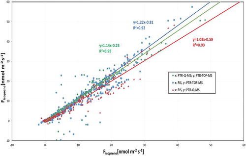
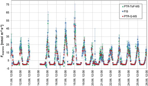
Figure 5. Isoprene fluxes measured with all three instruments during summer 2013. Random error estimates for FIS, PTR-ToF-MS and PTR-QMS flux data are shown as error bars and calculated for all three instruments as described in Section 2.4.5. The authors acknowledge the use of a similar figure in a conference paper/proceeding (see the ‘Acknowledgements’ section for more details).

In an approximation that is usually valid for a range of VMRs for which the instrument has been designed, a linear relationship between the VMR and the instrument response signal to this VMR is valid (see Figure 1):

Hence, VMR = a*X + b with X instrument signal VMR, a is the calibration factor and b is the calibration offset.

Comparing two different instruments, we can obtain

(2)

and a linear fit of VMR₁ against VMR₂ is influenced by both calibration factors a and calibration offsets b.

On the other hand, Figure 2 shows turbulent fluxes (f). These fluxes are approximated by the 30-minaverages of the covariance of the VMR with the vertical wind speed (w) as follows:

(3)

where VMR′  is the variation of VMR and w′  is the variation of w.

Comparing fluxes (i.e. making a linear fit), obtained with the same sonic anemometer – identical w′ – but different instrument VMRs it follows for a linear fit of f₁ vs. f₂:

• The offsets b of the instruments do not influence the fit at all.

• Differences in VMR₁ and VMR₂ play a role only when, at the same time, w′ is of significant size, i.e. big differences of VMRs do not influence the fit when w′ is close to zero.

It is therefore to be expected that the correlation coefficients (R²) are better for the measurements of fluxes (Figure 2) than for the measurements of VMR (Figure 1). In addition, a certain goodness of fit for VMR does not imply any goodness of fit for fluxes f.

From Figures 1 and 2 and Table 1, it can be concluded that the isoprene data generated by the three instruments are in good agreement. A 40% drift in the isoprene sensitivity was observed for the PTR-QMS during the 20 days’ intensive measurement period. Since this instrument was only calibrated at the beginning and the end of the 20 days’ intensive campaign, this drift is probably the cause of the small deviations in the PTR-QMS data. A major discrepancy is the offset in PTR-ToF-MS VMRs, which is mostly owned to the fact that this instrument observed higher isoprene levels at night (see also Figure 4). None of the instruments were automatically zeroed at night which may explain the discrepancies in the night-time data.

Figure 3. Average diurnal variations of VOCs (PTR-ToF-MS measurements), temperature and short wavelength radiation during the period of the PTR-ToF-MS measurements (11–26.06.2013). Error bars show the standard deviation on the average of the hourly means of the fluxes. ‘Hour of day’ is in UTC.

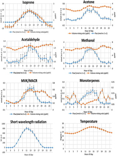
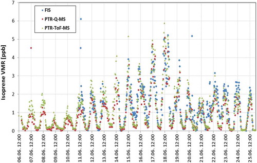
Figure 4. Isoprene volume mixing ratios (VMRs) measured with all three instruments in June 2013. Overall uncertainties for isoprene VMR measured with the two PTR-MS techniques are taken to be 10%. Overall uncertainties for isoprene VMR measured with FIS are taken to be 15%.

With PTR-ToF-MS, several VOCs were identified and measured in high enough VMRs to be relevant for further investigations (see Table 2).

Summary values/examples of fluxes/VMRs of several of the VOCs are shown in Table 3 and in Figure 3. Table 3 shows the averages of the diurnal fluxes and VMRs of several VOCs for which flux calculations could be performed during the measurement campaign. These fluxes show an average diurnal variation with a daytime peak that is more than three times the standard deviation of the night-time values that fluctuate around zero (see also examples in Figure 3 where that applied). Clearly, isoprene represents by far the largest input of carbon to the atmosphere, followed by methanol and monoterpenes that, in terms of carbon atoms, are almost identical.

The average diurnal variations of fluxes and VMRs are shown in Figure 3. The diurnal variations of the emissions of biogenic VOCs depend on leaf temperature and light (also shown in Figure 3), the emission factors have been found to be composed of, in general, a light-dependent and a light-independent fraction; the dependence on leaf temperature is exponential [42]. In addition, it should be mentioned that also environmental stresses affect biogenic VOC emissions. Some observations can be made based on the measured fluxes, VMRs and their diurnal variations (see later).

Figure 4 shows isoprene VMR in the forest. Isoprene was rather high during the campaign in June 2013 and could easily be measured by all three techniques, but with a difference, as seen in Figure 1.

Figure 5 shows that isoprene fluxes could easily be measured by all three techniques.

After presenting Tables 2 and 3 and Figures 1 and 5, the following additional observations could be made for the three VOC measurement techniques: PTR-ToF-MS, PTR-QMS and FIS.

PTR-ToF-MS. Large fluxes of isoprene were observed by PTR-ToF-MS with flux-values up to 53 nmol m⁻² s⁻¹ for isoprene, and with mean diurnal (24 h) flux of isoprene to be (5.20 ± 2.42) nmol m⁻² s⁻¹ (see Figures 3 and 5 and Table 3). We use the PTR-ToF-MS flux-data as the final results, because it was the instrument that was calibrated most frequently, measured with the highest Hz and provided most chemical details of the VOCs. The PTR-QMS and FIS flux-data are then used for validation and for comparison. A comparison of the three techniques can also be seen in Figures 1 and 2 and Table 1. The VMR of isoprene in the atmosphere measured by the PTR-ToF-MS was up to about 10 ppb, with a mean diurnal (24 h) average VMR of isoprene of (1.07 ± 0.53) ppb (see Figures 3 and 4 and Table 3).

PTR-QMS. Figure 5 shows that isoprene fluxes could also easily be measured with PTR-QMS; large fluxes of isoprene were observed by PTR-QMS with flux-values up to about 50 nmol m⁻² s⁻¹ for isoprene. Averaging 30 min of mass spectra that render flux calculations meaningless, but several other VOCs were identified/measured such a long averaging time by PTR-QMS during the summer campaign (protonated masses): mass 33 (methanol), mass 42 (acetonitrile), mass 43 (acetic acid and fragments/interferences), mass 45 (acetaldehyde), mass 59 (acetone), mass 61 (acetic-acid/methyl-formate), mass 73 (propionic-acid/methyl-ethyl-ketone/butanal), mass 87 (unknown), mass 89 (unknown), mass 93 (toluene), mass 107 (C8-alkyle-benzene), mass 137 (monoterpenes). Fluxes however could be only obtained for Isoprene, with a flux-value of isoprene up to about 50 nmol m⁻² s⁻¹, see also Figures 1 and 2 for comparison with the other techniques. The VMR of isoprene in the atmosphere measured by PTR-QMS was normally in the in range of 1–2 ppb during day-time summer (in June 2013), with a maximum value of around 8 ppb (see Figure 4). It should be mentioned, that for comparison, a short winter campaign was performed from 11.02.2013 until 08.03.2013 in the same forest with the PTR-QMS instrument. As expected, no isoprene fluxes were observed using PTR-QMS during these winter-time measurements.

FIS. Figure 5 shows that isoprene fluxes could also easily be measured with the FIS. Large fluxes of isoprene were also observed by FIS with flux-values up to 58 nmol m⁻² s⁻¹ for isoprene; see also Figures 1 and 2 for the comparison with the other techniques. The VMR of isoprene in the atmosphere measured by FIS was normally in range of 1–3 ppb during day-time in the summer 2013 (see Figure 4), with a maximum value of up to 10 ppb of isoprene.

3.2. Results and discussions of data obtained only by PTR-ToF-MS

In the following section, the results for several of the VOCs measured by PTR-ToF-MS are presented and discussed. The e-folding lifetimes and the parameters used for evaluating these are shown in Table 4.

Isoprene represents by far the largest input of carbon to the atmosphere among the species measured here (the largest input of biogenic VOC to the atmosphere) with flux-values up to 53 nmol m⁻² s⁻¹ for isoprene (by PTR-ToF-MS) and with mean diurnal (24 h) flux of isoprene to be (5.20 ± 2.42) nmol m⁻² s⁻¹. The maximum of the diurnal emission lies between the maxima of the short-wavelength radiation and of the temperature. The emission factor for isoprene has been found to have only a light-dependent component [42] and in fact, the flux measured at night is found to be zero. The measured isoprene VMR shows a diurnal variation similar to that of the flux and goes down to a value close to zero during the night, which can be explained by the short atmospheric residence time of this compound. VMRs of isoprene of up to 10 ppb were measured during summer 2013 by PTR-ToF-MS, with average/typical day-time values of 1–2 ppb, and with a mean diurnal (24 h) averages of VMR of isoprene of (1.07 ± 0.53) ppb. The main daytime loss mechanism is the reaction with OH, while during night, the reaction with the NO₃ radical can be important; the reaction with ozone is relatively slow [48] (see Table 4). Chemical degradation of isoprene within the canopy and in the layer between the top of the canopy and the measurement point will lead to some underestimation of the actual flux of isoprene. Schallhart et al. [24] found by model simulations of transport times and OH concentrations, at conditions very similar to those of the present study, that the loss of isoprene was likely to be between 3 and 5% (in Bosco Fontana, Lombardy, Italy).

Although horizontal wind speeds are generally low, at the height of the top of the tower average wind speeds are between 1.5 and 2 m s⁻¹, also transport of air masses may clearly have an influence on the observed VMRs.

Monoterpenes have been estimated to be the second largest source of biogenic VOC to the atmosphere at a global scale after isoprene [42,49]; however, in the Ispra forest they only make a relatively small contribution to the emissions of biogenic VOC to the atmosphere (Table 3), with a mean diurnal (24 h) flux of monoterpenes of (0.08 ± 0.05) nmol m⁻² s⁻¹. Monoterpenes have been found to be emitted by 46 families of flowering plants and in all conifers [50]. Their reactivity with respect to both OH and ozone as well as NO₃ radicals is high and the typical atmospheric lifetimes are even shorter than those of isoprene [48] (Table 4). Alpha-pinene is the monoterpene that is emitted in greatest abundance from vegetation followed by beta-pinene at temperate latitudes [49]. While for alpha-pinene both the reaction with OH and the reaction with ozone are important, for beta-pinene the reaction with OH dominates. Contrary to isoprene, the light-independent fraction of the emission is significant (e.g. in the case of alpha-pinene it is 40%, see Ref. [42]) and thus monoterpenes are also emitted at night. The diurnal variation of monoterpene fluxes shows a maximum in the afternoon. As with isoprene, the chemical degradation in the atmosphere between the point of emission and the measurement point leads to an underestimation of the actual VMR. Assuming, like in the case of isoprene, that the simulations made by Schallhart et al. [24] can be applied to the Ispra site, this underestimation will be between 5 and 15% in the case of alpha-pinene (which together with beta-pinene is likely to account for most of the monoterpene emissions in this forest). Beta-pinene reacts about 30% faster with OH, but slower with ozone (see Table 4), which leads to very similar atmospheric lifetimes. Monoterpene VMRs show a midday minimum, which must be explained by the fact that the VMR of the photo-chemically generated OH radicals typically reach a maximum by the middle of the day and thus also the removal rate of the monoterpenes by the reaction with OH is likely to reach a maximum and this apparently more than compensates for the increase in the emissions during the morning hours. At night, the reaction with the NO₃ radical, which is rapidly destroyed by photolysis during the day, may play an important role: The NO₃ radical is formed by the reaction between ozone and NO₂ and they are both found at relatively high concentrations throughout the night at the top of the tower. The calculated hourly rate of production of NO₃ radicals during the night is, in average, between a maximum of about 900 pptV in the early evening down to a minimum of approximately 550 pptV at 5 AM in the morning. It is therefore clear that with such high production rate of NO₃ radicals, it could be a significant sink for the terpenes, as the reaction rate constant with monoterpenes are generally very high.

Methanol is the third-most abundant input of carbon from biogenic VOC to the atmosphere [42,49], and its emissions show a seasonal variation with peaks in spring and autumn. Methanol is also produced by chemical reactions in the atmosphere and released from anthropogenic activities and biomass burning, but biogenic emissions are found to be its main source [51,52]. The light-dependent fraction of the flux is found to be 80% [42]. In this investigation, we found mean diurnal (24 h) fluxes of methanol to be (0.85 ± 0.41) nmol m⁻² s⁻¹. The removal of methanol from the atmosphere is mainly due to the reaction with OH radicals and dry deposition as well as wet deposition; globally the reaction with OH is the most important removal process, but deposition accounts for more than 40%, according to the model simulation by Tie et al. [53]. The relatively long lifetime of methanol implies that the compound is accumulated in the atmosphere and that the impact of the diurnal variations of the flux will be less evident than in the case of the more short-lived species. In fact, the VMR shows no visible relation to the flux from the canopy and thus the variations are likely to be explained by the influence of atmospheric transport. The flux has a maximum in the early afternoon and a minimum in the night; however, no significantly negative values are observed, so it appears that dry deposition of methanol at night is slow at the JRC-Ispra site, where there is normally very little turbulence in the atmosphere at night. The flux and VMR of methanol measured here are shown in Figure 3. The measured VMRs are within the range between the VMRs typically measured over forests and grasslands [51].

Acetone represents the fourth-most abundant emissions of carbon from biogenic VOC and the light-dependent fraction is 20% of the emissions [42,49]. It has the same PTR-signal as propanal, but emissions of propanal are known to be generally less than 10% of those of acetone [17]. The two main sources of acetone in the atmosphere, accounting for approximately equal contributions, have been found to be emissions from vegetation and oxidation of VOCs in the atmosphere [54,55]. The main removal pathway is the reaction with OH (see Table 4), but also photolysis (see Table 4) and deposition on land are of importance, there is a large exchange with the sea resulting in a slightly negative net flux from the atmosphere. Having a relatively long atmospheric lifetime (Table 4), acetone (like methanol) accumulates in the atmosphere and the impact of the diurnal variations of the flux is less evident than in the case of the more short-lived species. Taking into consideration that the degradation due to photolysis of acetone generally is slower than the reaction with the OH radical (see also Table 4), it can be expected that the atmospheric VMRs will show even less influence of the local emissions than in the case of methanol. The acetone flux has a maximum in the afternoon hours. The observed small variations of the measured VMRs are probably not related to the local emissions. As in the case of methanol, deposition at night is insignificant. Acetone measurements at the JRC-Ispra EMEP station during the years 1994–1995 were compared to measurements performed at several other European sites by Solberg et al. [56]. It was found that the VMRs measured in Ispra in 1994–1995 did not show the same variation during the year as the other rural stations that had a clear summertime maximum. A likely explanation for this could be that acetone VMRs at the Ispra site are influenced by local anthropogenic emissions. The VMRs reported by Solberg et al. [56] for the summer season (1.5–1.8 ppbV with 30 days running averages) are somewhat lower than those found in the present study (see Table 3).

Methacrolein and methylvinylketone (MACR and MVK) are the main products of the OH-initiated oxidation of isoprene with primary yields of 21 and 29%, respectively [57] in a NOx-containing atmosphere; for the relatively high NOx-concentrations at the Ispra site area this appears to be a reasonable estimate (see e.g. Ref. [15].). Both MACR and MVK have also been found in vehicle exhaust [58]. Two previous studies have indicated that MACR and/or MVK are also emitted directly by vegetation, while other studies have shown little or no such emissions (see Ref. [24], and references therein). The main atmospheric removal process is the reaction with the OH radical (see Table 4). Photolysis is not a significant loss process for MACR and only a minor loss process for MVK [59]. For MVK/MACR we found the mean diurnal (24 h) averages of VMR of MVK/MACR to be (0.42 ± 0.22) ppb and the mean diurnal (24 h) flux of MVK/MACR to be (0.06 ± 0.04) nmol m⁻² s⁻¹. The fluxes of MACR/MCR has a maximum at midday/early afternoon, at night they go to zero, but they never become negative. Comparing the isoprene and MACR/MVK fluxes in Figure 3, it can be seen that the peaks MACR/MVK fluxes are about 1.2% of the peak isoprene emissions. As mentioned above, for conditions very similar to the present study, Schallhart et al. [24] found that between 3 and 5% of the emitted isoprene would react with OH before reaching the measurement point; applying a chemical model to their system they find that the net yield of MVK and MACR would be 35% combined. Thus, using these findings of Schallhart et al. [24] to perform a rough evaluation of our data we can conclude that the observed flux of the sum of MACR and MVK is compatible with the assumption that oxidation of isoprene is the only significant source of this compound. The diurnal variation of MACR/MVK shows a maximum during daytime and in the early evening. The influence of the emissions from vegetation is clearly seen in the diurnal variation that shows a strong increase in the morning and midday hours, where MACR/MVK are produced from the reaction between isoprene and the OH radical; the high value in the evening must be explained by transport. The flux measurements show no deposition at night.

Acetaldehyde is an important component in the atmosphere. It acts as a source of ozone, peroxyacetylnitrate [60] and HOx radicals [61]. It is also a pollutant, and is classified as a hazardous air pollutant by the EPA [62]. There are several sources of atmospheric acetaldehyde, which include photochemical production as well as direct anthropogenic and natural emissions, but the relative importance of the different sources is poorly understood [63]. A recent investigation to improve our knowledge of acetaldehyde states that hydrocarbon oxidation provides the largest source of acetaldehyde [64]. As can be seen in Table 3, we found mean diurnal (24 h) averages of VMR of acetaldehyde of (1.59 ± 0.45) ppb and a mean diurnal (24 h) flux of acetaldehyde to be (0.10 ± 0.24) nmol m⁻² s⁻¹.

The main sink for acetaldehyde in the atmosphere is the reaction with the OH radical, with a small contribution from photolysis (see Table 4).

3.3. Comparison of the results obtained here with other studies

3.3.1 Comparison of the results found here with other studies of VOC VMRs and fluxes

Comparing of the VMRs and fluxes of the VOCs found in the present investigation with others studies in forests, vegetation-area, etc., is difficult because it depends on several parameters, e.g. the type of forest/trees/vegetation, time of the year, season, meteorology, weather during the measurement campaign, the measuring site set-up, tower height and also the types of different instruments used, etc.

As one of the scientific outcome of the study, several flux rates and their diurnal variations have been measured and compared to other studies, including the MEGAN model (reference 42 and 51 in the paper).

All of the comparisons with other studies are listed in Table 5 and discussed in Sections 3.3.2–3.3.6.

Table 5. Summary of the results obtained in this investigation and the comparison with other studies. Fluxes and VMR values for isoprene, acetone, acetaldehyde, methanol, MVK/MACR and monoterpenes.

	Isoprene	Acetone	Acet-ald.	Methanol	MVK/MACR	Monoterp.	Ref.
Flux (nmol m^−2 s^−1)
Average flux	5.20	0.13	0.10	0.85	0.06	0.08	This work
	6.466	0.335	0.228	1.168	0.314	0.209	[24]
	11.294*				0.119*		[23]
	0.3–1.2	0.9–2.2	1.1–2.3	3.2–3.8		0.5–1.8	[65]
	0.025	−0.013	0.133	1.655	0.041	1.235	[22]
	30.950**						[66]
	*Only day-time.
	**Only emission potential (basal emission rate).
VMR (in ppbV)
Average VMR	1.07	3.21	1.59	6.22	0.42	0.10	This work
	1.19				0.21		[23]
	0.10–0.14	1.0–2.1	0.4–1.3	1.6–3.5		0.1–0.3	[65]

3.3.2 Comparison of number of masses that showed a flux found here with other studies of VOC fluxes

In this investigation, we found about 10–20 (out of about 100 masses) that showed a flux (positive fluxes (emissions) and negative fluxes (depositions)). This number could e.g. be compared to the study of Schallhart et al. [24], in a similar forest: Bosco Fontana is a 233 ha forested nature reserve located in the northeast of the Po Valley, approximately 250 km from the Ispra site. The main tree species there are Quercus cerris (turkey oak), Quercus robur (pedunculate oak), Quercus rubra (northern red oak) and Carpinus betulus (hornbeam). For more details, see Ref. [24]. Schallhart et al. [24] found 29 (out of 163 masses) have a flux. Another study [22] found 494 (out of 664 masses) to have a flux. The measurements of Park et al. [22] were performed above an orange grove/field (direct flux measurement over an orange grove (orange plants/trees) in California’s Central Valley during the summer of 2010). Of course it all comes down to what criteria was used to define a flux: In the investigation presented here we use ‘fluxes that show an average diurnal variation with a daytime peak that was larger than three times the standard deviation of the night-time values that fluctuate around zero’, Schallhart et al. [24] used ≥3 sigma of noise (3 σ_noise) and Park et al. [22] used ‘fluxes when signal/noise ≥3’. Thus, our results are similar to the ones found by Schallhart et al. [24].

3.3.3 Comparison of VMR and flux values obtained for the most significant fluxes with values obtained from other studies

Comparisons with other studies can be found in Table 5.

We found isoprene to have the highest upwards fluxes. For isoprene in this investigation, we found mean diurnal (24 h) averages of VMR of isoprene to be (1.07 ± 0.53) ppb and mean diurnal (24 h) flux of isoprene to be (5.20 ± 2.42) nmol m⁻² s⁻¹.

In the study of Schallhart et al. [24], the flux of isoprene was found to be about 6.466 nmol m⁻² s⁻¹, in a ‘oak-forest’ similar to our measurement site. Therefore, the value is very similar to what we found in this investigation.

Kalogritis et al. [23] found 1.19 ppb for the VMR of isoprene (24 h average) in a Mediterranean oak forest in south-east France. That value is also very similar to what we found. The mean day-time flux (10:00–17:00) of isoprene was found to be 11.294 nmol m⁻² s⁻¹, which is about the double of what we found here, but it should be mentioned that the value from Kalogritis et al. [23] was only daytime.

Results from Davison et al. [65](a measurement campaign in May/June 2007, in a Mediterrenean coastal site at Castelporziano, 25 km south-west of Rome, Italy, in a Mediterranean macchia ecosystem). They found VMR to be in the range of 0.10–0.14 ppbV for isoprene. That value is lower to what we found. They found flux of isoprene to be in the range of 0.300–1.183 nmol m⁻² s⁻¹, which is lower to what we found here.

Park et al. [22] found a flux of isoprene to be only 0.025 nmol m⁻² s⁻¹, but the site was very different from ours, being an ‘orange grove’.

In a recent paper by Langford et al. [66], they investigated five European oak forests and found ‘isoprene emission potentials’ (basal isoprene emission rate) ranging from 0.175 nmol m⁻² s⁻¹ to 42.817 nmol m⁻² s⁻¹, including an ‘isoprene emission potential’ of 30.950 nmol m⁻² s⁻¹ for the JRC-Ispra forest, which is in agreement with the lower value found in this investigation for the isoprene flux. It should be mentioned that some of the FIS data in the present investigation were used, but none of the PTR-ToF-MS/PTR-QMS data presented here were used in the Langford et al.’s [66] study. Langford et al. [66] is about ‘isoprene emission potentials (also referred to as ’isoprene basal emission rate’ in the literature) in five European forests, whereas the paper presented here is about comparison of three instrumentations and values of VMR/fluxes for the following compounds (using PTR-ToF-MS): isoprene, terpenes, MVK/MeCR, methanol, acetone and acetaldehyde.

3.3.4 Comparison of VMR and flux of monoterpenes/sesquiterpenes with values obtained from other studies

Comparisons with other studies can be found in Table 5.

For the monoterpenes (C₁₀H₁₆) we found mean diurnal (24 h) averages for the VMR of the sum of monoterpenes to be (0.10 ± 0.09) ppb and the mean diurnal (24 h) flux of the sum of monoterpenes to be (0.08 ± 0.05) nmol m⁻² s⁻¹. In the study of Schallhart et al. [24], under similar conditions, the flux of monoterpenes was found to be about 0.209 nmol m⁻² s⁻¹, about twice what we found in the present investigation. Results from Davison et al. [65] showed VMR to be in the range of 0.13–0.30 ppbv for monoterpenes. That value is similar to what we found. They found flux of monoterpenes to be in the range of 0.489–1.753 nmol m⁻² s⁻¹, which is higher to what we found here.

Different conditions applied in the study by Park et al. [22] being an ‘orange grove’ and they found of net flux of 1.235 nmol m⁻² s⁻¹, which is much higher to what we found in the present investigation.

For the sesquiterpenes (C₁₅H₂₄) in the present investigation, we were around the detection limit of the PTR-ToF-MS instruments, so no significant values could be obtained for their VMRs and fluxes.

3.3.5 Comparison of VMR and flux of MVK/MACR with values obtained from other studies

Comparisons with other studies can be found in Table 5.

For MVK/MACR in this investigation, we found mean diurnal (24 h) averages of VMR of MVK/MACR to be (0.42 ± 0.22) ppb. Mean diurnal (24 h) flux of MVK/MACR to be (0.06 ± 0.04) nmol m⁻² s⁻¹. This can be compared to the study of Schallhart et al. [24], for similar conditions. Schallhart et al. [24] found the flux of MVK/MACR to be about 0.314 nmol m⁻² s⁻¹, which is significantly higher than what we found.

Kalogritis et al. [23] found 0.21 ppb of MVK/MACR (24 h average) in a Mediterranean oak forest in France, south-east France. That value is similar to what we found in the present investigation. They also found the mean day-time flux (10:00–17:00) of MVK/MACR to be 0.119 nmol m⁻² s⁻¹, which is higher to what we found here. Different conditions in the study by Park et al. [22] being in an ‘orange grove’, where they found of net flux of 0.041 nmol m⁻² s⁻¹, which is lower to what we found in the present investigation.

In our investigation, we found that the flux of MACR/MVK has a maximum at midday/early-afternoon, at night they go to zero, but they never become negative. Comparing the isoprene and MACR/MVK fluxes in Figure 3 it can be seen that the peaks of MACR/MVK fluxes are about 1.2% of the peak isoprene emissions. As mentioned previously, for conditions very similar to the present study, Schallhart et al. [24] found that between 3 and 5% of the emitted isoprene would react with OH before reaching the measurement point; applying a chemical model to their system they found that the net yield of MVK and MACR would be 35% combined. Thus, using these findings of Schallhart et al. [24] to perform a rough evaluation of our data here, we can conclude that the observed flux of the sum of MACR and MVK is compatible with the assumption that oxidation of isoprene is the only significant source of this compound.

The diurnal variation of the VMRs of MACR/MVK shows a maximum during daytime and in the early evening. The influence of the emissions from vegetation is clearly seen in the diurnal variation that shows a strong increase in the morning and midday hours, where MACR/MVK are produced from the atmospheric reaction between isoprene and the OH radical; the high value in the evening must be explained by transport.

The flux measurements of MACR/MVK show no deposition at night in the investigations here. This could be compared to the study of Schallhart et al. [24], where they only observe a small deposition of MACR/MVK.

3.3.6 A discussion of the fluxes of other oxygenated VOCs found in this investigation here and the comparison with other studies

Comparisons with other studies can be found in Table 5.

In the present investigation, here we found also other VOCs, e.g. the oxygenated VOCs, that were found to have had a significant measurable flux.

Methanol. In this investigation we found mean diurnal (24 h) flux of methanol to be (0.85 ± 0.41) nmol m⁻² s⁻¹, with a mean diurnal (24 h) averages for the VMR of methanol to be (6.22 ± 2.09) ppb. These results can be compared to Schallhart et al. [24] under similar conditions, where they also found significant amounts of methanol emitted from the forest, with a value of net flux of 1.168 nmol m⁻² s⁻¹, which is similar to our value. The results can also be compared to Davison et al. [65], where they also found significant amounts of methanol present and emitted from the forest, with a VMR value in the range of 1.6–3.5 ppbv for methanol, similar to what we found here, and with a value of net flux in the range of 3.210–3.815 nmol m⁻² s⁻¹ for methanol, which is higher than our value. Different conditions in the study by Park et al. [22], where they found a net flux of 1.655 nmol m⁻² s⁻¹ for methanol, which is higher than our value.

Acetone in this investigation we found mean diurnal (24 h) flux of acetone to be (0.13 ± 0.06) nmol m⁻² s⁻¹, with a mean diurnal (24 h) averages for the VMR of acetone to be (3.21 ± 1.17) ppb. The results can be compared to Schallhart et al. [24], where they also found significant amounts of acetone emitted from the forest, with a value of net flux of 0.335 nmol m⁻² s⁻¹, which is significant higher than our value. The results can also be compared to Davison et al. [65], where they also found significant amounts of acetone present and emitted from the forest, with a VMR value in the range of 0.96–2.1 ppbv for acetone, similar to what we found here, and with a value of net flux in the range of 0.861–2.152 nmol m⁻² s⁻¹ for acetone, which is significant higher than our value. Different conditions in the study by Park et al. [22], where they found a negative very small net flux of −0.013 nmol m⁻² s⁻¹ for acetone, which is of course much lower than our value.

For acetaldehyde in this investigation we found mean diurnal (24 h) averages of VMR of acetaldehyde to be (1.59 ± 0.45) ppb and mean diurnal (24 h) flux of acetaldehyde to be (0.10 ± 0.24) nmol m⁻² s⁻¹.

These results can be compared to Schallhart et al. [24], where they also found the amounts of acetaldehyde emitted from the forest, with a value of net flux of 0.228 nmol m⁻² s⁻¹, which is about twice our value. These results can also be compared to Davison et al. [65], where they also found significant amounts of acetaldehyde present and emitted from the forest, with a VMR value in the range of 0.44–1.3 ppbv for acetaldehyde, similar to what we found here, and with a value of net flux in the range of 1.135–2.270 nmol m⁻² s⁻¹ for acetaldehyde, which is also significant higher than our value. Under different conditions in the study by Park et al. [22], they found a net flux of 0.133 nmol m⁻² s⁻¹, which is similar to our value.

4 Conclusions

In summarising the above results and discussions, we can conclude the following.

For what we believe was the first time, we used three different instrumentations: PTR-ToF-MS, PTR-QMS and FIS in parallel to measure VOC VMRs and fluxes. Figures 1–5 show that all three instrumentations could measure some of the VOC VMRs and fluxes, and the three instruments were in good agreement. We present here the PTR-ToF-MS flux-data for this paper and use them as the final results, because it was the instrument that was calibrated most frequently, measured with the highest Hz and the instrument that provided most chemical details of the VOCs. We have used the PTR-QMS and FIS flux-data only for validation and for comparison.

Tables 2 and 3 show that about 20 VOCs were clearly identified by PTR-ToF-MS and fluxes could be achieved for many of them: We found isoprene to be the one with the highest upwards flux. For isoprene we found a mean diurnal (24 h) VMR of (1.07 ± 0.53) ppb and a mean diurnal (24 h) flux (5.20 ± 2.42) nmol m⁻² s⁻¹. These values are generally in agreement with other studies under similar ‘forest’ conditions (see e.g. Refs. [23,24]), but higher when e.g. comparing to a ‘orange glove’ [22]. For the monoterpenes (C₁₀H₁₆), we found mean diurnal (24 h) averages of VMR of (0.10 ± 0.09) ppb for the monoterpenes and mean diurnal (24 h) flux of (0.08 ± 0.05) nmol m⁻² s⁻¹ for the monoterpenes. The flux of the monoterpenes measured here is in reasonable agreement with other studies (see e.g. Refs. [24,65]). For MVK/MACR (oxidation products from the primary emitted compound isoprene), we found mean diurnal (24 h) averages of VMR of MVK/MACR to be (0.42 ± 0.22) ppb. Mean diurnal (24 h) flux of MVK/MACR is (0.06 ± 0.04) nmol m⁻² s⁻¹. Our flux value is lower than the ones by Kalogritis et al. [23] and Schallhart et al. [24], but higher than the one by Park et al. [22]. We measured also other VOCs, e.g. several oxygenated VOCs, that had a significant flux. The following mean diurnal (24 h) averages for the VMR and the mean diurnal (24 h) fluxes were found: methanol – (6.22 ± 2.09) ppb and (0.85 ± 0.41) nmol m⁻² s⁻¹; acetone – (3.21 ± 1.17) ppb and (0.13 ± 0.06) nmol m⁻² s⁻¹; and acetaldehyde – (1.59 ± 0.45) ppb and (0.10 ± 0.24) nmol m⁻² s⁻¹. Both methanol and acetone have a relatively long atmospheric lifetime and for this reason, there is no evident relationship between the local fluxes and the observed VMRs. The acetone VMRs are clearly higher than those observed at other rural sites. A previous study [56] concludes that the acetone VMRs in Ispra probably are influenced by local anthropogenic sources.

Author contributions

NRJ, CG and IG organised the campaign at JRC-Ispra, Italy. MM and AW performed the measurements with the PTR-ToF-MS instrument. NRJ, CG and IG performed the measurements with the PTR-QMS instrument. CG and IG performed the measurements with the FIS instrument. CG, MM and JH performed the statistical evaluation of the data. NRJ and JH prepared the manuscript with contributions from all co-authors to the manuscript/data-evaluation.

Acknowledgments

The authors thank Silvano Fares for his support. The authors also acknowledge that part of the material in the present paper has been used in a conference paper/proceeding (ref. [67]): N.R. Jensen, C. Gruening, I. Goded, M. Müller, O. Pokorska, A. Cescatti, J. Hjorth and A. Wisthaler, Eddy-covariance flux measurements in a forest using PTR-ToF-MS, PTR-Q-MS, FIS and other instrumentations, 7th International Conference on Proton Transfer Reaction Mass Spectrometry and its Applications in Environmental Science, February 14th−19th, Obergurgl, Austria, pp. 34–37 (2016) Link: https://www.uibk.ac.at/iup/buch_pdfs/9783903122000.pdf.

Disclosure statement

No potential conflict of interest was reported by the authors.

Appendix 1

The meteorological data at tower top in four figures.

Figure A1a. Temperature at the tower top in June 2013 during the measurement campaign.

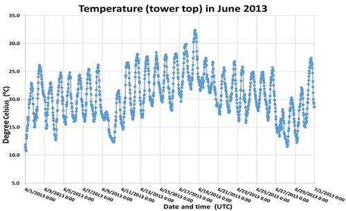
Figure A1b. Relative humidity at the tower top in June 2013 during the measurement campaign.

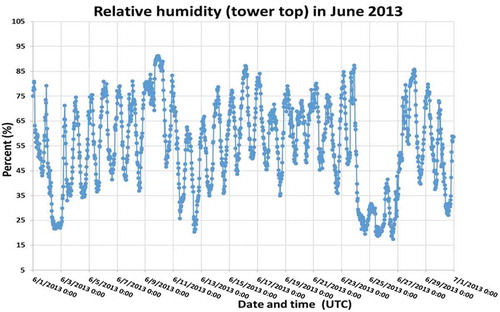
Figure A1c. Wind speed at the tower top in June 2013 during the measurement campaign.

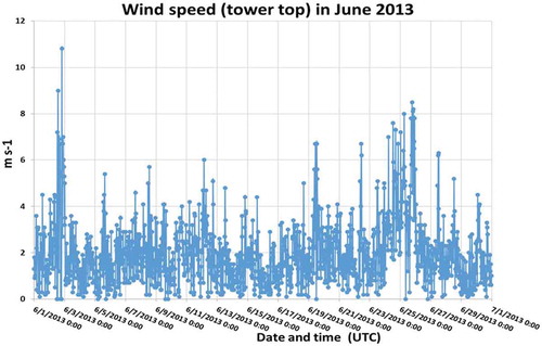
Figure A1d. Solar radiation at the tower top in June 2013 during the measurement campaign.

Appendix 2

Meteorological data from year 2013, from a nearby EMEP/GAW station (within 500 m).

Figure A2. Solar global irradiation, precipitation amount, and temperature monthly means observed at the EMEP/GAW measuring station in the JRC-Ispra in 2013, compared to the 1990–1999 period ± standard deviations (the Figure is from the ref. EUR report [15]).

Appendix 3

Multi-component VOC calibration mixture for calibration of PTR-ToF-MS/PTR-QMS.

Table A3. Multi-component calibration mix. (an 11-component VOC standard mixture from Apel-Riemer Environmental Inc., Denver, USA). Uncertainty is a conservative estimate of the combination of the uncertainties of the gravimetric preparation and analysis.

Compounds	Conc./VMR (ppb)	Uncertainties
Acetaldehyde	1084	±5%
Methanol	1015	±5%
Isoprene	1040	±5%
Acetone	1003	±5%
Acetonitrile	994	±5%
Methyl Ethyl Ketone	1001	±5%
Benzene	1045	±5%
Toluene	1023	±5%
m-Xylene	980	±5%
alfa-Pinene	1008	±5%
1,3,5-Trimethylbenzene	961	±5%

Appendix 4

Detection limits for the PTR-ToF-MS.

Table A4. Detection limits for the PTR-ToF-MS: Exemplary results from a PTR-ToF-MS calibration performed on 06.06.2013 for all of the VOCs measured in this investigation is shown here. ‘ncps’ is an abbreviation for “normalised counts per second (normalised to 10⁶ cps of (H₂O)H⁺ and (H₂O)₂H⁺ ions). Limits of detection (LOD, 2 s) and precision (1 s) values were calculated for a 0.1 s signal integration time.

		Sensitivity		Precision at
Compounds	m/z	(ncps ppbV^−1)	LOD (ppbV)	About 20 ppbV
Methanol	33.034	11.1	1.36	2.86
Acetonitrile	42.0344	20.1	0.33	1.27
Acetaldehyde	45.034	13.9	1.04	2.44
Acetone	59.0497	18.1	0.34	1.26
Isoprene	69.0704	8.4	0.43	1.98
2-Butanone	73.0653	15.2	0.32	1.99
Benzene	79.0548	10.0	0.29	1.70
Toluene	93.0704	11.2	0.26	1.58
m-Xylene	107.0861	12.2	0.20	1.47
1,3,5-Trimethylbenzene	121.1017	12.5	0.22	1.84
Alfa-pinene	137.133	5.2	0.61	2.92

References

- B. Finnlayson-Pitts and J. Pitts Jr., Chemistry of the Upper and Lower Atmosphere,San Diego, California (Academic Press, 2000).
- S.D. Piccot, J.J. Watson and J.W. Jones, J. Geophys. Res. 97, 9897 (1992). doi:10.1029/92JD00682.
- C. Guenther, N. Hewitt, D. Erickson, R. Fall, C. Geron, T. Graedel, P. Harley, L. Klinger, M. Lerdau, W.A. Mckay, T. Pierce, B. Scholes, R. Steinbrecher, R. Tallamraju, J. Taylor and P. Zimmerman, J. Geophys. Res. 100, 8873 (1995). doi:10.1029/94JD02950.
- K. Sindelarova, C. Granier, I. Bouarar, A. Guenther, S. Tilmes, T. Stavrakou, J.-F. Müller, U. Kuhn, P. Stefani and W. Knorr, Atmos. Chem. Phys. 14, 9317 (2014). doi:10.5194/acp-14-9317-2014.
- K. Ito, P. Kinney and G.D. Thurston, Inhalation Toxicol. 7, 735 (1995). doi:10.3109/08958379509014477.
- K. Ito and G.D. Thurston, J. Expo. Anal. Environ. Epidemiol. 6, 79 (1996).
- K. Ito, S.F. De Leon and M. Lippmann, Epidemiology 16, 446 (2005). doi:10.1097/01.ede.0000165821.90114.7f.
- M. Kanakidou, J.H. Seinfeld, S.N. Pandis, I. Barnes, F.J. Dentener, M.C. Facchini, R. Van Dingenen, B. Ervens, A. Nenes, C.J. Nielsen, C.E. Swietlicki, J.P. Putaud, Y. Balkanski, S. Fuzzi, J. Hjorth, G.K. Moortgat, R. Winterhalter, C.E.L. Myhre, K. Tsigaridis, E. Vignati, E.G. Stephanou and J. Wilson, Atmos. Chem. Phys. 5, 1053 (2004). doi:10.5194/acp-5-1053-2005.
- M. Hallquist, J.C. Wenger, U. Baltensperger, Y. Rudich, D. Simpson, M. Claeys, J. Dommen, N.M. Donahue, C. George, A.H. Goldstein, J.F. Hamilton, H. Herrmann, T. Hoffmann, Y. Iinuma, M. Jang, M.E. Jenkin, J.L. Jimenez, A. Kiendler-Scharr, W. Maenhaut, G. McFiggans, T.F. Mentel, A. Monod, A.S.H. Prevot, J.H. Seinfeld, J.D. Surratt, R. Szmigielski and J. Wildt, J. Atmos. Chem. Phys. 9, 5155 (2009). doi:10.5194/acp-9-5155-2009.
- EPA, Health, Particulate Matter, Air & Radiation, US EPA (EPA. Gov. 2010).
- T. Novakov and J.C. Penner, Nature. 365, 823 (1993).
- R. Vingarzan, Atmos. Environ. 38, 3431 (2004). doi:10.1016/j.atmosenv.2004.03.030.
- R. Van Dingenen, F.J. Dentener, F. Raes, M.C. Krol, L. Emberson and J. Cofala, Atmos. Environ. 43, 604 (2009). doi:10.1016/j.atmosenv.2008.10.033.
- M.J. Hollaway, S.R. Arnold, A.J. Challinor and L.D. Emberson, Biogeosciences 9, 271 (2012). doi:10.5194/bg-9-271-2012.
- J.-P. Putaud, P. Bergamaschi, M. Bressi, F. Cavalli, A. Cescatti, D. Daou, A. Dell’Acqua, K. Douglas, M. Duerr, I. Fumagalli, I. Goded, F. Grassi, C. Gruening, J. Hjorth, N.R. Jensen, F. Lagler, G. Manca, S. Martins Dos Santos, M. Matteucci, R. Passarella, V. Pedroni, O. Pokorska and D. Roux, JRC-Ispra Atmosphere–Biosphere–Climate Integrated Monitoring Station. 2013 Report, (EUR 26995 EN, JRC93069, 2014).
- M. Graus, A. Hansel, A. Wisthaler, C. Lindinger, R. Forkel, K. Hauff, M. Klauer, A. Pficher, B. Rappengück, D. Steigner and R. Steinbrecher, Atmos. Env. 40, S43 (2006). doi:10.1016/j.atmosenv.2005.09.094.
- J. De Gouw and C. Warneke, Mass. Spectrom. Rev. 26, 223 (2007). doi:10.1002/mas.20119.
- R. Taipale, T.M. Ruuskanen, J. Rinne, M.K. Kajos, H. Hakola, T. Pohja and M. Kulmala, Atmos. Chem. Phys. 8, 6681 (2008). doi:10.5194/acp-8-6681-2008.
- M. Müller, M. Graus, T.M. Ruuskanen, R. Schnitzhofer, I. Bamberger, L. Kaser, T. Titzmann, L. Hörtnagl, G. Wohlfart, T. Karl and A. Hansel, Atmos. Meas. Tech. 3, 387 (2010). doi:10.5194/amt-3-387-2010.
- T. Karl, P. Harley, L. Emmons, B. Thornton, A. Guenther, C. Basu, A. Turnipseed and K. Jardine, Science 330, 816 (2010). doi:10.1126/science.1192534.
- T.M. Ruuskanen, M. Müller, R. Schnitzhofer, T. Karl, M. Graus, I. Bamberger, L. Hörtnagl, F. Brilli, G. Wohlfart and A. Hansel, Atmos. Chem. Phys. 11, 611 (2011). doi:10.5194/acp-11-611-2011.
- J.H. Park, A.H. Goldstein, J. Timkovsky, S. Rares, R. Weber, J. Karlik and R. Holzinger, Science 341, 643 (2013). doi:10.1126/science.1235053.
- C. Kalogridis, V. Gros, R. Sarda-Esteve, B. Langford, B. Loubet, B. Bonsang, N. Bonnaire, E. Nemitz, A.-C. Genard, C. Boissard, C. Fernandez, E. Ormeño, D. Baisnée, I. Reiter and J. Lathière, Atmos. Chem. Phys. 14, 10085 (2014). doi:10.5194/acp-14-10085-2014.
- S. Schallhart, P. Rantala, E. Nemitz, D. Taipale, R. Tillmann, T.-F. Mentel, B. Loubet, G. Gerosa, A. Finco, J. Rinne and T.M. Ruuskanen, Atmos. Chem. Phys. 16, 7171 (2016). doi:10.5194/acp-16-7171-2016.
- W. Lindinger, A. Hansel and A. Jordan, Chem. Soc. Rev. 27, 347 (1998). doi:10.1039/a827347z.
- W. Lindinger, A. Hansel and A. Jordan, Int. J. Mass. Spectrom. Ion Proc. 173, 191 (1998). doi:10.1016/S0168-1176(97)00281-4.
- B. D’Anna, A. Wisthaler, Ø. Andreasen, J. Viidanoja, N.R. Jensen, C.J. Nielsen, A. Hansel, J. Hjorth and Y. Stenstrøm, J. Phys. Chem. A 109, 5104 (2005). doi:10.1021/jp044495g.
- M. Müller, T. Milkoviny, W. Jud, B. D’Anna and A. Wisthaler, Chemometrics Intell. Lab. Syst. 127, 158 (2013). doi:10.1016/j.chemolab.2013.06.011.
- M. Graus, M. Müller and A. Hansel, J. Am. Soc. Mass. Spec. 21, 1037 (2010). doi:10.1016/j.jasms.2010.02.006.
- A. Jordan, S. Haidacher, G. Hanel, E. Hartungen, L. Märk, H. Seehauser, R. Schottkowsky, P. Sulzer and T.D. Märk, Int. J. Mass Spectrom. 286, 122 (2009). doi:10.1016/j.ijms.2009.07.005.
- A. Wisthaler, N.R. Jensen, R. Winterhalter, W. Lindinger and J. Hjorth, Atm. Env. 35, 6181 (2001). doi:10.1016/S1352-2310(01)00385-5.
- E.P. Hunter and S.G. Lias, J. Phys. Chem. Reference Data 27, 413 (1998). doi:10.1063/1.556018.
- H. Westberg, B. Lamb, R. Hafer, A. Hills, P. Sherson and C. Vogel, J. Geophys. Res. 106, 24347 (2001). doi:10.1029/2000JD900735.
- A.J. Hills and P.R. Zimmerman, Anal. Chem. 62, 1055 (1990). doi:10.1021/ac00209a017.
- T. Titzmann, M. Graus, M. Müller, A. Hansel and A. Ostermann, Int. J. Mass. Spectrom. 295, 72 (2010). doi:10.1016/j.ijms.2010.07.009.
- T.G. Karl, C. Spirig, J. Rinne, C. Stroud, P. Prevost, J. Greenberg, R. Fall and A. Guenther, Atmos. Chem. Phys. 2, 279 (2002). doi:10.5194/acp-2-279-2002.
- R.T. McMillen, Meteorology 43, 231 (1988).
- L. Hörtnagl, R. Clement, R.M. Graus, A. Hammerle, A. Hansel and G. Wohlfart, Atm. Env. 24, 2024 (2010). doi:10.1016/j.atmosenv.2010.02.042.
- M. Göckede, T. Foken, M. Aubinet, M. Aurela, M. Banza. et al. Biogeosciences. 5, 433 (2008). doi: 10.5194/bg-5-433-2008
- R. Kormann and F.X. Meixner, Boundary Layer Meteorol. 99, 207 (2001). doi:10.1023/A:1018991015119.
- Guidance for the Demonstration of Equivalence of Ambient Air Monitoring Methods, EC. Working Group 15, Jan. 2010: http://ec.europa.eu/environment/air/quality/legislation/pdf/equivalence.pdf
- A.B. Guenther, X. Jiang, C.L. Heald, T. Sakulyanontvittaya, T. Duhl, L.K. Emmons and X. Wangh, Geosci. Model Dev. 5, 1471 (2012). doi:10.5194/gmd-5-1471-2012.
- B. Finlayson-Pitts and J.N. Pitts Jr., Atmospheric Chemistry: Fundamentals and Experimental Techniques (J. Wiley and Sons, New York, Chichester, Brisbane, Toronto and Singapore, 1986).
- R. Atkinson, D.L. Baulch, R.A. Cox, J.N. Crowley, R.F. Hampson, R.G. Hynes, M.E. Jenkin, M.J. Rossi and J. Troe, Atmos. Chem. Phys. 6, 3625 (2006). doi:10.5194/acp-6-3625-2006.
- R. Atkinson, J. Phys. Chem. 26, 215 (1997).
- R. Atkinson, S.M. Aschmann, A.M. Winer, M. Arthur and J.N. Pitts, Int. J. Chem. Kinet. 13, 1133 (1981). doi:10.1002/kin.550131104.
- M.T.B. Romero, M.A. Blitz, D.E. Heard, J. Pilling, B. Price, P.W. Seakins and L. Wang, Faraday Discuss 130, 73 (2005). doi:10.1039/b419160a.
- J.D. Fuentes, M. Lerdau, R. Atkinson, D. Baldocchi, W. Bottenheim, P. Ciccioli, B. Lamb, C. Geron, L. Gu, A. Guenther, T.D. Sharkey and W. Stockwell, Bull. Am. Meteorological Soc. 81, 1537 (2000). doi:10.1175/1520-0477(2000)081<1537:BHITAB>2.3.CO;2.
- P. Messina, J. Lathière, K. Sindelarova, N. Vuichard, C. Granier, J. Ghattas, A. Cozic and D.A. Hauglustaine, Atmos. Chem. Phys. 16, 14169 (2016). doi:10.5194/acp-16-14169-2016.
- M. Lerdau, J. Whitbeck and N.M. Holbrook, Trends Ecol. Evol. 6, 201 (1991). doi:10.1016/0169-5347(91)90019-T.
- B.G. Heikes, W. Chang, M.E.Q. Pilson, E. Swift, H.B. Singh, A. Guenther, D.J. Jacob, B.D. Field, R. Fall, D. Riemer and L. Brand, Global Biogeochemical Cycle 16, 80–81 (2002). doi:10.1029/2002GB001895.
- T. Stavrakou, A. Guenther, A. Razavi, L. Clarisse, C. Clerbaux, P.F. Coheur, D. Hurtmans, F. Karagulian, M. De Maziere, C. Vigouroux, C. Amelynck, N. Schoon, Q. Laffineur, B. Heinesch, M. Aubinet, C. Rinsland and J.-F. Muller, Atmos. Chem. Phys. 11, 4873 (2011). doi:10.5194/acp-11-4873-2011.
- X. Tie, A. Guenther and E. Holland, Geophys. Res. Lett. 30, 1881 (2003). doi:10.1029/2003GL017167.
- D.J. Jacob, B.D. Field, E.M. Jin, I. Bey, Q. Li, J.A. Logan, R.M. Yantosca and H.B. Singh, J. Geophys. Res. A. 107, ACH 5–1 (2002).
- E.V. Fischer, D.J. Jacob, D.B. Millet and R.M. Yantosca, J. Mao, Geophys. Res. Lett. 39, L01807 (2012).
- S. Solberg, C. Dye, N. Schmidbauer, et al., J. Atmos. Chem. 25, 33 (1996). doi:10.1007/BF00053285.
- E.C. Tuazon and R. Atkinson, Int. J. Chem. Kinet. 22, 1221 (1990). doi:10.1002/kin.550221202.
- T.A. Biesenthal, Q. Wu, P.B. Shepson, et al., Atmos. Environ. 31, 2049 (1997). doi:10.1016/S1352-2310(96)00318-4.
- T. Gierczak, J.B. Burkholder, R.K. Talukdar, A. Mellouki, S.B. Barone and A.R. Ravishankara, J. Photochem. Photobio. A: Chem. 110, 1 (1997). doi:10.1016/S1010-6030(97)00159-7.
- J.M. Roberts, Atmos. Environ. 24A, 243 (1990). doi:10.1016/0960-1686(90)90108-Y.
- H.B. Singh, M. Kanakidou, P.J. Crutzen and D.J. Jacob, Nature 378, 50 (1995). doi:10.1038/378050a0.
- EPA, Chemical Summary for Acetaldehyde, EPA (749-F-94-003a. Office of Pollution Prevention and Toxics, 1994).EPA, Washington DC, United States of America.
- H.B. Singh, L.J. Salas, R.B. Chatfield, E. Czech, A. Fried, J. Walega, M.J. Evans, B.D. Field, D.J. Jacob, D. Blake, B. Heikes, R. Talbot, G. Sachse, J.H. Crawford, M.A. Avery, S. Sandholm and H. Fuelberg, J. Geophys. Res. 109, D15S07 (2004).
- D.B. Millet, A. Guenther, D.A. Siegel, N.B. Nelson, H.B. Singh, J.A. De Gouw, C. Warneke, J. Williams, G. Eerdekens, V. Sinha, T. Karl, F. Flocke, E. Apel, D.D. Riemer, P.I. Palmer and M. Barkley, Atmos. Chem. Phys. 10, 3405 (2010). doi:10.5194/acp-10-3405-2010.
- B. Davison, R. Taiplae, B. Langford, P. Misztal, S. Frares, G. Matteucci, F. Loreso, J.N. Cape, J. Rinne and C.N. Hewitt, Biogeosciences 6, 1655 (2009). doi:10.5194/bg-6-1655-2009.
- B. Langford, J. Cash, W.J.F. Acton, A.C. Valach, C.N. Hewitt, S. Fares, I. Goded, C. Gruening, E. House, A.-C. Kalogridis, V. Gros, R. Schafers, R. Thomos, M. Broadmeadow and E. Nemitz, Biogeosciences 14, 5571 (2017). doi:10.5194/bg-14-5571-2017.
- N.R. Jensen, C. Gruening, I. Goded, M. Müller, O. Pokorska, A. Cescatti, J. Hjorth and A. Wisthaler Conference paper/proceeding: Eddy-covariance flux measurements in a forest using PTR-ToF-MS, PTR-Q-MS, FIS and other instrumentations, 7th International Conference on Proton Transfer Reaction Mass Spectrometry and its Applications in Environmental Science, February 14th −19th, Obergurgl, Austria, pp 34–37 (2016) Link: https://www.uibk.ac.at/iup/buch_pdfs/9783903122000.pdf.