Multilevel analysis of bulk shipping fleet productivity: a big data approach

ABSTRACT

Fleet productivity is an important element in shipping economics, a defining factor in the asset’s profitability, and a key driver of the emission footprint of the industry. This paper analyzes the productivity of bulk vessels in a multi-dimensional framework by utilizing over 800,000 voyages data which were carried out by 17,764 vessels over a 7-year horizon and was derived from the Automated Identification System. An examination of the underlying factors driving transportation output provides further understanding of how the operational behaviours impact vessel productivity. The insights from this research have important implications for policy making in investment, operational enhancement, and emission reduction.

KEYWORDS:

• Productivity
• bulk shipping
• fleet
• AIS
• tonne-mile
• laden ratio

1. Introduction

Stopford (2009) defines fleet productivity as tonne-miles, that is, cargo weight multiplied by laden distance traveled, supplied per vessel capacity. Fleet productivity is perhaps the most important term to understand shipping economics, but still it is interesting to see that in many analyses the term is assumed constant over time (Wijnolst and Wergeland 1996, 313). This situation unfortunately has not significantly improved in the literature so far. There are many factors that determine fleet production, such as the load factor, waiting days, sailing speed, and the ballast distance (Stopford 2009). The inadequacy of in-depth research on the topic is mainly due to the opacity in the way the shipping industry operates, specifically the lack of voyage-specific cargo information (Adland, Jia, and Strandenes 2017).

This research aims at shedding light by investigating the fleet productivity of the global bulk shipping fleet at the vessel level along multiple dimensions. The principal research questions are—are there variations in bulk fleet productivity by vessel class, trade regions, and time? and what drives the fleet transport output? This research outlines a framework for measuring fleet productivity using real-time vessel operational data which is primarily derived from the Automatic Identification System (AIS). The employment of Multi-level Mixed Models (MLMM) in interpreting the multi-level factors that influence fleet productivity expands our understanding of clustered data analysis which characterizes such micro-level asset utilization data.

The contributions to the literature are threefold. Firstly, productivity KPI measurements for the vessels are constructed by employing actual vessel operational data in terms of sailing distance and time spent at ports, among other factors derived from AIS. Secondly, the variation in productivity KPIs by vessel class, trade region and time is investigated using the robust modelling techniques of MLMM. Thirdly, the drivers of transport tonne-mile output are analysed with the former mentioned elements being accounted for.

2. Literature review

Shipping productivity was initially studied in the context of increased transport capacity and sailing speed as the result of technological advancement, such as the invention of steel hull and steam engine (North 1958, 1968; Harley 1988). Wijnolst and Wergeland (1996) introduced the theoretical framework in modern fleet productivity analysis, essentially measuring how efficient the vessel capacity could be used to cover the distances necessary to meet transport demand. The proportion of the vessel capacity being utilized for cargo payload, i.e. vessel capacity utilization is one of the key factors in measuring fleet productivity. The capacity utilization has typically been assumed to be constant in early studies, see, for instance, Endresen et al. (2004) and Endresen et al. (2007). More recently, the voyage-dependent variation in vessel capacity utilization has been recognized (Adland and Jia 2018) because load factor can be affected by contracted cargo amount, port infrastructure, or the available vessel size.

Vessel sailing speed and port turnaround time affect how quickly a vessel completes the transportation task. Sailing speed is affected by weather (Zis, Psaraftis, and Ding 2020), fuel price (Cariou 2011), and contractual terms (Adland and Jia 2019a), and thus has been studied as regards speed optimisation (Aydin, Lee, and Mansouri 2016) and energy saving (Adland et al. 2017; Jia et al. 2017). Ports being the connecting nods in the supply chain, their turnaround time is an important factor in port operational efficiency (Kennedy et al. 2011), performance management (Dayananda and Dwarakish 2020), and congestions (Bai, Jia, and Xu 2021).

Despite efforts in studying the different related aspects affecting fleet productivity, these Key Performance Indicators (KPI) have not been investigated jointly with regards to the variations in vessel class and trades. Moreover, the literature so far has treated laden and ballast voyages indifferently. Thanks to micro-level vessel tracking data based on the AIS, this paper now is able to provide an in-depth investigation in this domain.

The remainder of the paper is organized as follows. Section 3 introduces fleet productivity KPIs. Section 4 illustrates the data. Section 5 explains the MLMM methodology. Section 6 illustrates the empirical modelling and reports the results of the investigation on fleet productivity variation by multiple dimensions. Section 7 reports the analytic results on what drives fleet transport output. A discussion of implications is presented in Section 8, which is followed by concluding remarks in Section 9.

3. Bulk shipping fleet productivity KPIs

3.1. Fleet productivity

In the framework defined by Wijnolst and Wergeland (1996), eight factors that affect the fleet productivity:

1. Average speed

2. Ballast factor, defined as the average number of miles in ballast relative to miles in loaded conditions

3. Waiting days per trip at ports, incl. time for loading and unloading

4. Trips per month

5. Average length of haul, that is, the average number of nautical miles sailed in loaded condition

6. Load factor, defined as total cargo size (tonnes) per DWT

7. Share of total fleet in lay-up or idle

8. Months off hire per year

The latter two factors (share of total fleet in lay-up or idle; months off hire) are not measured in the current setup, as they are based primarily on exogeneous circumstances such as vessels’ technical conditions, retrofitting needs and the longer-term market outlook. Load factor can be estimated based on the AIS draught information (Jia, Prakash, and Smith 2019) and a non-linear relationship between load factor and vessel size has been detected in the literation (Adland, Jia, and Strandenes 2018). The reliability of AIS draught information in cargo size estimation yet needs further investigation especially for heterogeneous cargos, as suggested in Adland, Jia, and Strandenes (2017). In this paper, we opt out the focus on load factor and leave it for future research.

A voyage starts at the time of leaving the last discharge port (or, potentially, a drydock following repairs or maintenance) with a ballast leg to the load port, followed by a laden leg to the discharge port. Figure 1 illustrates two such voyages performed by two vessels at different times. In the case of Voyage 1 the vessel was open in port Galveston, US, and the next contract is to load in port Bonaire, Caribbean, and discharge in Qingdao, China. In the case of Voyage 2, the vessel was open in port Fukuyama, Japan, and the next contract is to load in port Cape Town, South Africa, and discharge in port Villanueva, Mexico. From a productivity point of view, the main difference between Voyage 1 and 2 is the proportion of the distance that the vessel sailed ballast (from open port to load port) in comparison to laden (from load to discharge port).

Figure 1. Example of shipping voyages.

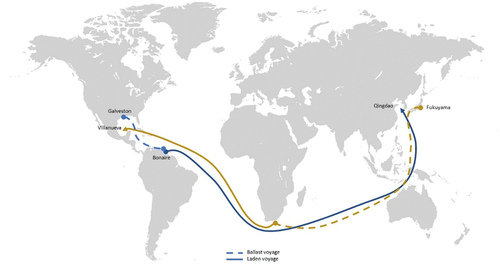
There are three components of the voyage time: time spent when transporting the cargo, time spent when positioning to pick up the cargo; and time spent at ports either waiting to be served or cargo handling (loading and discharging). Let total voyage time be

(1) $\mathbf{V}{\mathbf{T}}_{\mathbf{i},\mathbf{j}}=\mathbf{D}{\mathbf{l}}_{\mathbf{i},\mathbf{j}}/\mathbf{v}{\mathbf{l}}_{\mathbf{i},\mathbf{j}}+\mathbf{D}{\mathbf{d}}_{\mathbf{i},\mathbf{j}}/\mathbf{v}{\mathbf{d}}_{\mathbf{i},\mathbf{j}}+{\mathrm{\Pi }}_{\mathbf{i},\mathbf{j}}$(1)

where

$\mathrm{V}{\mathrm{T}}_{\mathrm{i},\mathrm{j}}$ is the total voyage time spent by vessel i during voyage j;

$\mathrm{D}{\mathrm{l}}_{\mathrm{i},\mathrm{j}}$ is the sailing distance while laden for vessel i during voyage j;

$\mathrm{D}{\mathrm{b}}_{\mathrm{i},\mathrm{j}}$ is the sailing distance while ballast for vessel i during voyage j.

$\mathrm{v}{\mathrm{l}}_{\mathrm{i},\mathrm{j}}$ is the vessel sailing speed when laden, that is, sail to the discharge port with cargo onboard, by vessel i for voyage j;

$\mathrm{v}{\mathrm{b}}_{\mathrm{i},\mathrm{j}}$ is the vessel i sailing speed in ballast, that is, positioning to the load port, by vessel i for voyage j;

${\mathrm{\Pi }}_{\mathrm{i},\mathrm{j}}$ is the time spent at both loading and discharging port by vessel i for voyage j.

For a given cargo circulated in the market, the laden distance is effectively fixed as it is determined by the requirements of the buyer or seller of the cargo (depending on trade terms). The transportation contract typically also stipulates the sailing speed, either directly for the laden leg or indirectly by stipulating the date by which the vessel must present herself for loading (the laycan), see, for instance, Adland and Jia (2019a). Consequently, the proportion of a voyage’s laden distance to its total distance (the laden ratio) becomes a measure of how productive the vessel is in that voyage. In the following subsections, the KPIs are introduced.

3.2. Productivity KPI

Three dynamic factors are the key drivers of fleet productivity: utilization of vessel capacity, the ballast distance and port turnaround time. Jia, Prakash, and Smith (2019) have suggested ways to estimate cargo payload using the Automatic Identification System (AIS) draught data. However, the reliability of the draught data field in AIS is of varying quality. In this paper, the focus is on the latter two Key Performance Indicators (KPI) for fleet productivity: the laden ratio and port turnaround time. Specifically, the laden ratio accounts for both speed and time spent in the laden leg during the voyage.

(2) ${\mathbf{\Lambda }}_{\mathbf{i},\mathbf{j}}=\mathbf{D}{\mathbf{l}}_{\mathbf{i},\mathbf{j}}/\left(\mathbf{D}{\mathbf{l}}_{\mathbf{i},\mathbf{j}}+\mathbf{D}{\mathbf{b}}_{\mathbf{i},\mathbf{j}}\right)$(2)

where ${\mathrm{\Lambda }}_{\mathrm{i},\mathrm{j}}$ is the laden ratio for vessel i during voyage j.

4. Data

The dataset, kindly provided by the company Signal Ocean,¹ is primarily derived from the Automatic Identification System for collision avoidance and vessel tracking. The dataset includes details for 837,865 voyages performed by 17,764 vessels from January 2014 to October 2020. Each row in the dataset refers to a single voyage from the start (open) port, via the load port to the discharge port, with the associated distances, coordinates, and timestamps (i.e. the vessel arrival and departure for each port). The world geography is categorized into eight regions, and the number of countries within each region is in brackets: Africa (35), Arabian Gulf (9), East Coast Americas (34), Europe (49), Far East (5), Oceania (16), South East Asia (13), and West Cost Americas (13). Vessels are classified by the type of vessel and its size. There are seven vessel classes for dry bulk carriers and six vessel classes for oil tankers. Vessel specifications, such as DWT and age, are obtained from the Clarksons World Fleet Registry database by matching the vessel identity (IMO number) for each voyage.

To summarize, the comprehensive dataset includes information along three dimensions, including

1. Spatial: the geographic locations when the vessel is open for the next shipment (open port), the load, and discharge port.

2. Asset type: the vessel size, type, age, and identity of the asset.

3. Temporal: the date and hour for each voyage (start and end), the duration of time spent both at sea and at ports (loading and discharging).

5. Multi-level mixed models

Owing to the characteristics in the dataset, the voyage observations can be clustered by vessel class to reflect demand for its transportation service. Voyages can also be clustered geographically by load and discharge regions to reflect the impact of geography and international trade economics. Finally, as the observations are across 7 years, there might be time cluster effect. In order to properly account for the clustered data structure, a Multilevel Mixed Effect model (MLMM) is applied in the analysis. The core of MLMM is that it can recognize and incorporate the variance presented both in the overall sample and in the clusters (Hedeker and Gibbons 2006). In other words, the models allow random intercept and slope estimates across clusters. These coefficients consequently become random variables following a distribution. The MLMM has gained popularity in social studies in order to address the dependency or correlation among observations within the same group.

Consider a three-level MLMM, in which each individual level1 observation i (i.e. a voyage performed by a vessel) can be clustered into level2 j groups (vessel classes), and further cross-classified into level3 k clusters (trading routes). The relationships in this multilevel model structure can be stated as follows:

Level_1 model:

(3) ${\mathbf{y}}_{\mathbf{i}\mathbf{j}\mathbf{k}}={\alpha }_{\mathbf{j}\mathbf{k}}+{\beta }_{\mathbf{j}\mathbf{k}}\cdot {\mathbf{X}}_{\mathbf{i}\mathbf{j}\mathbf{k}}+{\epsilon }_{\mathbf{i}\mathbf{j}\mathbf{k}}$(3)

where ${\mathrm{y}}_{\mathrm{i}\mathrm{j}\mathrm{k}}$ is the dependent variable observed for unit i, that belongs to clusters j and k;

${\mathrm{X}}_{\mathrm{i}\mathrm{j}\mathrm{k}}$ is the independent variable vector for unit i;

${\alpha }_{\mathrm{j}\mathrm{k}}\mathrm{a}\mathrm{n}\mathrm{d}{\beta }_{\mathrm{j}\mathrm{k}}$ are the intercepts and slopes, which are variable by clusters;

Here, ${\alpha }_{ik}\hspace{0.17em}$and ${\beta }_{jk}$ can be seen as random variables that can be further explained by a fixed component and random effects that are dependent on cluster j, that is, the Level 2 structure:

Level_2 model:

(4) ${\alpha }_{\mathrm{j}\mathrm{k}}={\theta }_{00\mathrm{k}}+{\mathrm{b}}_{0\mathrm{j}}$(4)

(5) ${\beta }_{jk}={\theta }_{10k}+b_{1j}$(5)

where ${\theta }_{00k}$ and ${\theta }_{10k}$ represent fixed components in the intercept and slope, respectively, that do not vary across cluster j (c.f. the disappearance of subscript j) but may vary across cluster k, and

$b_{0jk}$ and $b_{1jk}$ represent the random components in the intercept and slope that vary by cluster j.

Finally, the Level 3 structure can be stated as

Level_3 mode

(6) ${\theta }_{00\mathrm{k}}={\gamma }_0+{\mathrm{c}}_{00\mathrm{k}}$(6)

(7) ${\theta }_{10k}\hspace{0.17em}={\gamma }_1\hspace{0.17em}+c_{10k}$(7)

where ${\gamma }_0$ and ${\gamma }_1$ are fixed components in the intercept and slope, for the level3 cluster k;

$c_{00k}$ and $c_{10k}$ are the random components which vary by cluster k.

Thus, the equations (3)(3) ${\mathbf{y}}_{\mathbf{i}\mathbf{j}\mathbf{k}}={\alpha }_{\mathbf{j}\mathbf{k}}+{\beta }_{\mathbf{j}\mathbf{k}}\cdot {\mathbf{X}}_{\mathbf{i}\mathbf{j}\mathbf{k}}+{\epsilon }_{\mathbf{i}\mathbf{j}\mathbf{k}}$(3) - (7(7) ${\theta }_{10k}\hspace{0.17em}={\gamma }_1\hspace{0.17em}+c_{10k}$(7) ) can be combined in a form of:

(8) ${\mathbf{y}}_{\mathbf{i}\mathbf{j}\mathbf{k}}={\gamma }_0+{\mathbf{b}}_{0\mathbf{j}}+{\mathbf{c}}_{00\mathbf{k}}+\left({\gamma }_1+{\mathbf{b}}_{1\mathbf{j}}+{\mathbf{c}}_{10\mathbf{k}}\right)\cdot {\mathbf{X}}_{\mathbf{i}\mathbf{j}\mathbf{k}}+{\epsilon }_{\mathbf{i}\mathbf{j}\mathbf{k}}$(8)

Therefore, the coefficient estimates have one set of estimates for each cluster. The models are estimated using Maximum Likelihood method.

Model (8) is also referred as a partial pooling model (PPM), representing the notion of pooled information from all the observations with consideration of cluster variances in the slope and intercept (${\tau }_0^2$ and ${\tau }_1^2$).

Note that if no cluster variances in slope or intercept are considered (that is, ${\propto }_j$ and ${\beta }_j$ are equal to zero) then Eq. (3)(3) ${\mathbf{y}}_{\mathbf{i}\mathbf{j}\mathbf{k}}={\alpha }_{\mathbf{j}\mathbf{k}}+{\beta }_{\mathbf{j}\mathbf{k}}\cdot {\mathbf{X}}_{\mathbf{i}\mathbf{j}\mathbf{k}}+{\epsilon }_{\mathbf{i}\mathbf{j}\mathbf{k}}$(3) becomes a simple linear regression:

(9) ${\mathbf{y}}_{\mathbf{i}\mathbf{j}}=\alpha +\beta \cdot {\mathbf{X}}_{\mathbf{i}\mathbf{j}}+{\epsilon }_{\mathbf{i}\mathbf{j}}$(9)

Model (9) is referred as a Complete Pooling model (CPM), that is, all the observations are from one single pool without any clusters. In this setting all the information from the observations is combined together and a single regression line is fitted for the whole dataset, with no consideration of any clustering structure.

The third model is to fit a separate regression for each cluster:

(10) ${\mathbf{y}}_{\mathbf{i}\mathbf{j}}=\alpha +{\beta }_{\mathbf{j}}\cdot {\mathbf{X}}_{\mathbf{i}\mathbf{j}}+{\epsilon }_{\mathbf{i}\mathbf{j}}$(10)

where ${\beta }_{\mathrm{j}}$ estimates are slopes within each cluster j.

Model (10) is referred as a No Pooling model (NPM), where none of the information from other clusters is combined or pooled together to fit the regression. Only information within the cluster is utilized to estimate the cluster-slopes. This model is equivalent to fitting dummy variables.

Combined, the above models allow the investigation of the presence of between/within clusters variances in the model parameters (either intercept or slope). In terms of model selection, the Bayesian Information Criterion (BIC), which is a penalized-likelihood criterion that attempts to trade off accuracy and parsimony in order to find the best-fit model, is used.

In the following subsections, the research question is whether fleet productivity, as measured by the Laden ratio ${\mathrm{\Lambda }}_{i,j}$ and port time ${\mathrm{\Pi }}_{i,j}$, differs by (i) vessel class, (ii) load region, and (iii) time-year effects. In essence, equation (8)(8) ${\mathbf{y}}_{\mathbf{i}\mathbf{j}\mathbf{k}}={\gamma }_0+{\mathbf{b}}_{0\mathbf{j}}+{\mathbf{c}}_{00\mathbf{k}}+\left({\gamma }_1+{\mathbf{b}}_{1\mathbf{j}}+{\mathbf{c}}_{10\mathbf{k}}\right)\cdot {\mathbf{X}}_{\mathbf{i}\mathbf{j}\mathbf{k}}+{\epsilon }_{\mathbf{i}\mathbf{j}\mathbf{k}}$(8) is estimated with independent variables and random intercepts are the focus. In each subsection, three models are estimated: (a) MLMM model by estimating a fixed intercept (average productivity KPIs) and cluster-variant random intercepts; (b) Complete pooling model (CPM) by only allowing for a fixed intercept for all the observations; and (c) No pooling model (NPM) by estimating separate intercepts for each cluster.

6. Variations in productivity KPIs

The fleet productivity variations across vessel class, geography, and time are analyzed using MLMM take into account the clustering structure in the data and allow for variance within and between clusters. Figure 2 presents the density plots of the two productivity KPIs: Laden ratio ${\mathrm{\Lambda }}_{i,j}$ and port time ${\mathrm{\Pi }}_{i,j}$. The laden ratio ${\mathrm{\Lambda }}_{i,j}$ has an average value of 63% and median value of 57.6%. The port time ${\mathrm{\Pi }}_{i,j}$ has average value of 10.5 days and median value of 8.65 days.

Figure 2. Density plots of laden ratio and port time.

6.1. Variation by vessel class

Each vessel nests within a vessel class and, as shown in Table 2, the dataset covers voyages undertaken by 13 vessel classes. For oil tankers, the vessel class ranges from the 300,000+ DWT VLCC which transport crude oil exclusively to 30,000 DWT MR1 (Medium Range) tankers which transport oil products. For dry bulk carriers, vessels range from the 270,000+ DWT VLOC, which are built to transport iron ore exclusively, to 30,000 DWT Handysize vessels which can carry a variety of dry bulk cargo (e.g. cement, phosphate, grains, or steel products).

Table 1. Model estimation statistics, by vessel class.

Laden ratio	N(obs)	ll(null)	ll(model)	df	AIC	BIC
MLMM^a	837,865	.	209617	3	−419229	−419194^a
CPM	837,865	171464	171464	1	−342925	−342913
NPM (dummy)	837,865	171464	209679	13	−419332	−419180
Port time
MLMM^a	837,865		−2788608	3	5577221	5577256^a
CPM	837,865	−2829765	−2829765	1	5659531	5659543
NPM (dummy)	837,865	−2829765	−2788547	13	5577119	5577271

The table reports the post estimation results of the three model specifications for two KPIs (laden ratio and port time).

MLMM assumes there is within-cluster and between-cluster variance in the KPI.

CPM assumes there is neither within nor between variance in the KPI.

NPM assumes there is only within-cluster variance in the KPI.

^arepresents that the model is chosen based on BIC.

Table 2. MLMM estimation results for KPIs by vessel class.

Mixed-effects ML regression		Number of Obs. = 837,865
		Obs. per group
Group variable	Vessel class	min	=	5,154
Number of groups	13	avg	=	64,451.20
		max	=	143,652
	Part A: Laden ratio	Part B: Port time
Fixed effects
Intercept	0.6019***	10.1939***
	(0.0163)	(0.5668)
Random-effects Parameters
Vessel class: Identity
var(_cons)	0.0035***	4.1752***
	(0.0014)	(1.6351)
Log likelihood = 209617.36		Log likelihood = −2788607.6

This table reports the MLMM estimation results for the fixed intercept and variance in random intercepts in the levels.

***represents the estimation is statistically significant at 99% confidence.

Numbers in bracket () are standard errors.

The section on Random-effects Parameters report the variance of the random intercepts by vessel class.

The estimates of the random intercepts are presented in Figure 3.

Table 1 reports the post-estimation statistics, including Akaike’s information criterion (AIC) and Bayesian information criterion (BIC), degrees of freedom (df), and log likelihood (ll) for the constant-only model (null) and the model. The best fitted model is chosen based on BIC, which is defined as $-2logL+p\left(log\left(n\right)\right)$ where L is the maximized value of the likelihood function of the model in-use, n is the sample size, and p is the number of parameters estimated by the model. Therefore, a lower BIC value suggests a better model fit. As a result, MLMM provides the best fit, suggesting the presence of random intercepts by vessel class.

Table 2 reports the estimation results of the MLMM for the two KPIs by vessel class. As shown, the estimated fixed intercept is 60.19% and 10.2 days for laden ratio and port time, respectively. The random-effects parameters reported the variance in random intercepts by vessel class, which are 0.35% and 4.2 days for laden ratio and port time, respectively. Random intercept estimates per vessel class are presented in the form of Table 6. Figure 3 presents the MLMM estimation of the two KPIs (laden ratio and port time) by vessel class. The bar chart represents the laden ratio (LHS) variation and the line represents the port time (RHS) variation by vessel class.

Figure 3. Laden ration and port time variation by vessel class (The dots represent the random intercept estimates, whose upper and lower value is marked by two times of standard deviation of the estimations).

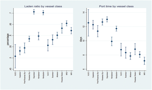
The first observation is that there is a cluster-driven estimation difference in the intercept of both laden ratio and port time by vessel class. Moreover, the variation within class is different as well. When sorting by size, there appears a clear trend in the KPIs across the vessel classes. Overall, larger vessels (VLOC, Capesize, post-Panamax dry, VLCC) have lower laden ratio compared to the smaller vessel sizes. This result is expected as large vessels such as VLOC or Capesize bulk carriers engage in long-haul international trades with less flexibility in cargo types and destinations. Thus, most of the vessels sail laden to the discharging region (for example, China) and sail in ballast back to the origin (for example, Brazil) for the next load. Conversely, small vessels are more involved in regional trades with greater flexibility in both routes and cargo types for carriage. Therefore, smaller vessels are better utilized in terms of the laden ratio.

Larger vessels spend longer port time as the cargo handling time is typically longer for larger vessels. VLOC has the highest port time at 12.5 days, which includes anchoraging and berthing, while MR1 vessels have the lowest port time at 7.2 days. The results also show that tankers have faster turnaround time in ports compared to dry bulkers by 3.76 days. Faster cargo handling techniques using pipe and pump for liquid products may partially explain the difference. Less congested oil tanker terminals compare to dry bulker terminals may also be another factor.

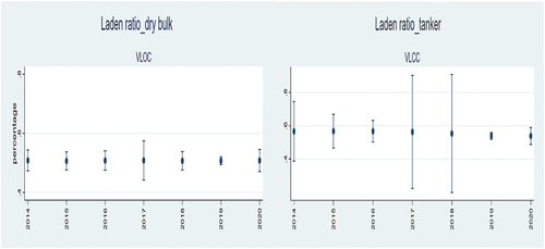
6.2. Variation by year

In this section, time is added as an additional level, facilitating the investigation of annual variation in productivity KPIs by vessel class. Three models are estimated, and the post estimation statistics BIC, MLMM suggest the existence of both between- and within-year variance in the KPIs.

The MLMM Maximum Likelihood estimated KPI by year is presented in Figure 4 (laden ratio) and Figure 5 (port time) for selective vessel classes due to limited space, the graphs for other vessel classes are available upon request. The results show, interestingly, that over the 7-year sample period, there are no significant changes in the two KPI means across the years, but large variance is shown in the tanker fleet laden ratio in 2017 and 2018. The result suggests relative stability in operations for most vessel classes, on average, during this time frame, while the tanker segment shows higher volatility in the KPIs periodically.

Figure 4. Laden ratio variation by vessel class and year.

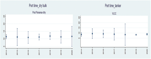
Figure 5. Port time variation by vessel class and year.

6.3. Variation by vessel class and trade region

In a global economy, each region and nation are involved in different levels of trade. Geography is a significant constraint to transport in the real world since it trades space for time and money (Rodrigue 2020). Oceangoing vessels spatially link the geographic regions which generate the supply and demand of commodities. There is a spatial distribution of resources, population, and economic activities. Consequently, regional economic and physical features have a direct impact on maritime voyages. In this section, the question is whether spatial maritime transportation demand is correlated with the variation in the fleet productivity by vessel class. Geography is closely aligned with the types of commodities being exported (for example, iron ore from Brazil): it has an impact on the length of the trip and the state of regional infrastructure may affect cargo handling efficiency.

The estimation results for the KPIs by vessel class and trade region are firstly reported in Table 3. The fixed intercept estimates are 0.698 and 12.31 for laden ratio and port time, respectively. The results also suggest there is variances in both KPIs in the levels. Variance in the trade region level appears to be higher than in the vessel class level. Overall, the results show a large variation in the KPIs across trade region. In fact, the variance in the estimated random intercept for both KPIs is larger for the trade region cluster level than (variance of 0.0135) for the vessel class cluster level (0.0053), respectively. This suggests that, within the vessel classes, there is significant dissimilarity of the KPIs across trade routes. For instance, VLCC laden ratio ranges from 30% to 90% and Handysize laden ratio ranges from 53% to 93%. Overall, the lowest laden ratio occurs in intra-regional trades, and this is understandable as intra-regional trades are short-distanced and the voyages have higher probability for lower laden ratio. On the other hand, most of the voyages with high laden ratio are loaded in the Far East region for many of the vessel classes. The estimated random intercepts in laden ratio are presented in Figure 6.

Figure 6. Laden ratio variation by vessel class and trade region.

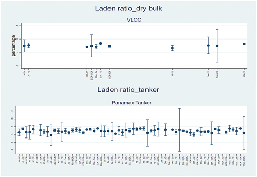
Table 3. MLMM estimation results for KPIs by vessel class and trade region.

Mixed-effects ML regression		Number of Obs. = 837,865
		Observations per group
Group variable	No. of groups	Minimum	Average	Maximum
Vessel class	13	5,154	64,451.20	143,652
Trade region	716	1	1,170.20	34,020
	Part A: Laden ratio		Part B: Port time
Intercept	0.6980***		12.3128***
	(0.0208)		(0.6338)
Random-effects Parameters
Vessel class: Identity
var(_cons)	0.0053***		4.9518***
	(0.0024)		(2.0425)
Trade region: Identity
var(_cons)	0.0135***		10.0385***
	(0.0008)		(0.6129)
Log likelihood = 209617.36			Log likelihood = −2788607.6

This table reports the MLMM estimation results for the fixed intercept and variance in random intercepts in the levels.

***represents the estimation is statistically significant at 99% confidence level.

Numbers in bracket () are standard errors.

The section on Random-effects Parameters reports the variance of the random intercepts by year & vessel class.

The estimates of the random intercepts are presented in Fig. 9 to Fig. 12 (and Fig. 9(2) – Fig. 12(2) in the Appendix).

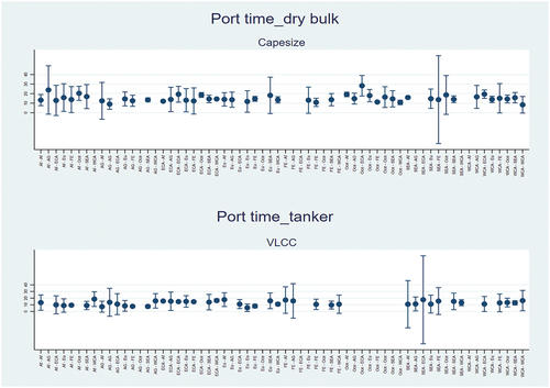
The estimated random intercepts in port time for selective vessel classes are presented in Figure 7. Again, variance across trade regions is observed in each vessel class. It is apparent that Africa, SE Asia, and EC Americas appear frequently in trade regions with longest port time for many vessel classes. Far East and WC Americas are among the regions with shortest port time. The difference between the maximum and minimum port time can be as high as 22.3 days within the Handymax vessel class, of which the maximum port time is 29.3 days in the SE Asia—Africa trade and 7 days in intra-Far East trade. The between cluster port time difference is even higher: 25.6 days difference between Handymax (maximum 29.3 days) and MR1 (minimum 3.69 days).

Figure 7. Port time variation by vessel class and trade region.

7. The explanatory factors of fleet transport output tonne-miles

In this section, the investigation is taken a step further by analyzing the relationship between the fleet tonne-mile output and key operational factors, including laden ratio, port time, ballast speed and laden speed, and their relative importance. The annual output per vessel is calculated using Eq. (5)(5) ${\beta }_{jk}={\theta }_{10k}+b_{1j}$(5) based on the 837,865 voyages that were carried by 17,764 unique vessels during 2014–2020. The dataset is then winsorized by excluding the top and bottom one-percentile. This results in a dataset with 98,393 annual observations of vessel transport output (tonne miles).

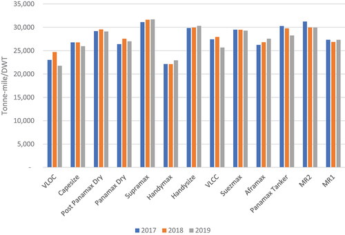
By definition, a vessel’s tonne-mile output is a product of the cargo transported (tonne) and laden distance (mile) over a period. For a given time t (consisting of sailing time and port time), the total laden distance for a vessel is a function of average speed (both laden and ballast speed), total time spent at ports, and the laden distance ratio. The final model, thus, include four explanatory variables in the MLMM, which is estimated using maximum likelihood by allowing for variations in coefficient estimations within and cross clusters. Figure 8 presents the tonne-mile/DWT output per vessel class in 2017–2019.

Figure 8. Transport output ton-mile/dwt by vessel class.

Table 4 reports the estimation results of the MLMM. The variables are z-scores scaled by standardizing each observation around its mean and standard deviation ($\frac{x_i-\bar{x}}{\sigma }$). Panel A reports the coefficient estimates for the four explanatory variables. Panel B reports the variance estimates of the cluster-dependent coefficients. The results show that all the four variables are statistically significant at 99% confidence level. More importantly, the results show that ballast speed is the most important factor in explaining the tonne-mile output (coefficient estimate of 3.86) comparing to the other variables. Laden speed is determined mostly by the charter party terms (Adland and Jia, 2019a, b) and there is a financial incentive to deliver the cargos on time and fast (Lindstad and Eskeland 2015; Yang, Zhang, and Ge 2022), as situations allow. On the other hand, the vessel operator and captain has relatively more flexibility to vary her ballast speed based on market situations, such as the urgency of the next voyage or saving fuel consumption by sailing slow.

Table 4. MLMM estimation results for tonne-mile transport output.

Mixed-effects ML regression		Number of Obs. = 98,393
Group variable: vessel class		Observations per group
No. of groups: 13		Minimum	Average	Maximum
		1,151	7,568	18,055
	Coef.	Std. Err.	[95% Conf.	Interval]
Laden ratio	0.18586***	(0.0489)	0.08993	0.28180
Port time	−0.09282***	(0.0195)	−0.13112	−0.05453
Laden speed	0.27604***	(0.0693)	0.14025	0.41182
Ballast speed	3.86459***	(0.7113)	2.47046	5.25873
Constant	0.27753	(0.2558)	−0.22392	0.77897
Random-effects Parameters
Vessel class: Identity
var(Laden ratio)	0.03092	(0.0126)	0.01391	0.06872
var(Port time)	0.00489	(0.0019)	0.00225	0.01065
var(Laden speed)	0.06195	(0.0248)	0.02829	0.13562
var(Ballast speed)	6.50456	(2.5751)	2.99384	14.13211
var(Constant)	0.85062	(0.3338)	0.39422	1.83543
var(Residual)	0.18341	(0.0008)	0.18180	0.18504
LR test vs. linear model: chi2(5) = 1.2e + 05 Prob > chi2 = 0.0000

This table reports the MLMM estimation results for the fixed coefficients and variance in random slope in the levels.

***represents that the estimation is statistically significant at 99% confidence level.

Numbers in bracket () are standard errors.

The section on Random-effects Parameters reports the variance in the random coefficients by vessel class.

Port time, being negatively related to tonne-mile, bears the least weight in the relationship. As expected, the laden distance ratio and laden speed are positively correlated with tonne-mile output, and their weights are far less important the ballast speed. The results also show there is variation in the coefficient estimates across the vessel class clusters. The relationship of ballast speed and tonne-mile output shows the largest variance across clusters compared to other variables.

8. Discussion and implications

This research aims at understanding the difference in vessel productivity across vessel class, trade region and time by utilizing the micro-level AIS vessel tracking data. It also provides further evidence on the impact factors on transport tonne-mile output. Variations in the KPIs are detected across vessel class and trade regions, considering the characteristics in vessel type and its corresponding trade.

Large vessels such as VLOC and VLCC are found to have a 51% and 56% laden ratio, respectively, on average over the 2014–2020 sample period. Smaller vessels such as Supramax and Handysize in the dry bulk segment had a laden ratio of above 70%, and MR2 in the tanker segment had laden ratio of 65%. Given that the low laden ratio for large vessels is a result of their limited flexibility in terms of trading pattern and cargoes carried, a key question is whether there are ways to improve the laden ratio fundamentally through transportation network design. One direction might be to improve cargo-vessel matching efficiency and optimal route planning (Papageorgiou et al. 2014).

With regards to port time, after considering vessel size clusters, the results show a large variation by trade regions. For instance, voyages serving trade regions SE Asia—Africa had the longest port time on average for two vessel classes (Handymax and Handysize) with above 29 days compared to 7 days in intra-Far East trades. The results also show that, for instance, a VLOC vessel may spend less than 12 port days on an Oceania—Far East voyage, which is 1 week shorter than for an EC Americas—SE Asia voyage. There are two key aspects in relation to port time variance: cargo handling efficiency and the traffic volume. The former is dependent on the port infrastructure and port management, which is particularly hard to observe from the current data and methodology.

The analysis of the drivers of transport output reveals further evidence of generalized and vessel class-specific patterns. The directions, negative or positive, of the explanatory variables are mostly as expected. Most importantly, the findings suggest that the ballast speed is the dominating factor in explaining the tonne-mile output of vessels, supporting earlier results in the literature suggesting that the ballast leg is the only part of the voyage where vessel operators have the flexibility to adjust sailing speed (Adland and Jia 2018), as opposed to the laden leg which is mostly governed by contractual terms.

The international shipping industry has a reputation of opacity due to, in part because the execution of each voyage represents a complex interplay between multiple stakeholders (for example, owners, charterers, sub-charterers, cargo owners, port agents, technical managers, pool operators, and so on). From a top-down level, this research assists in improving the transparency of global shipping operations by providing a voyage-based multilevel investigation of the efficiency of the international tramp shipping fleet over the past 7 years. This potentially has great societal value. For instance, tonne-mile output is one of the two parameters in calculating carbon intensity (gram of CO₂ per tonne-mile) for transportation assets. Consequently, the implication for policymakers is that the IMO’s proposal of data collection system to determine the required annual operation carbon intensity indicator (CII) should not only take the vessel’s productivity into account but also find the balancing point of optimal productivity with low emissions. With sustainable development high on the agenda, improving productivity should be the ultimate focus for all stakeholders.

9. Concluding remarks

The results from this research point to the conclusion that the fleet productivity and transport output are crucially dependent on each voyage’s laden ratio and port turnaround, as well as sailing speed, particularly ballast speed. The results of this study suggest that the utilization of shipping assets is essentially dependent on better information and execution in terms of ship and cargo matching, ship-terminal scheduling and efficient cargo handling in port. The objective of such actions is clearly to minimize the unproductive distance (ballast distance) and waiting time in the maritime supply chain.

The limitations of the study arise from the insufficient inclusion of certain information. Foremost, the lack of access to cargo information limits the research to account for cargo payload in the KPIs. Moreover, exogenous variables such as extreme weather conditions, which can have a decisive impact on the port time KPI, may explain the variations in productivity. Future research should consider the tradeoff between transportation output (tonne-mile production) and transportation cost or emissions by incorporating the time-varying speed during a voyage, and therefore the dynamic relationship between fuel cost and vessel speed. With access to detailed cargo size data, the dependency of DWT utilization on vessel size, trade region, and time should also be considered.

Disclosure statement

No potential conflict of interest was reported by the author.

Additional information

Funding

The work was supported by the Norwegian Research Council, under the project “Smart Digital Contracts and Commercial Management” (project number: 280684).

Notes

1. https://www.thesignalgroup.com.

References

- Adland, R., G. Fonnes, H. Jia, O. D. Lampe, and S. P. Strandenes. 2017. “The Impact of Regional Environmental Regulations on Empirical Vessel Speeds.” Transportation Research Part D 53: 37–49. doi:10.1016/j.trd.2017.03.018.
- Adland, R., and H. Jia. 2018. “Dynamic Speed Choice in Bulk Shipping.” Maritime Economics & Logistics 20: 253–266. doi:10.1057/s41278-016-0002-3.
- Adland, R., and H. Jia 2019a. “Contract Barriers and Energy Efficiency in the Crude Oil Supply Chain.” Proceedings of the IEEE International Conference on Industrial Engineering and Engineering Management 2018, Bangkok, Thailand.
- Adland, R., and H. Jia 2019b. “Smart Contracts and Demurrage in Ocean Transportation.” Second International Symposium on Foundation and Applications of Blockchain (FAB), April 5, Los Angeles, USA.
- Adland, R., H. Jia, and S. P. Strandenes. 2017. “Are AIS-Based Trade Volume Estimates Reliable? The Case of Crude Oil Exports.” Maritime Policy & Management 44 (5): 657–665. doi:http://dx.doi.org/10.1080/03088839.2017.1309470.
- Adland, R., H. Jia, and S. P. Strandenes. 2018. “The Determinants of Vessel Capacity Utilization: The Case of Brazilian Iron Ore Export.” Transportation Research Part A 110: 191–201. doi:10.1016/j.tra.2016.11.023.
- Aydin, N., H. Lee, and A. Mansouri. 2016. “Speed Optimization and Bunkering in Liner Shipping in the Presence of Uncertain Service Times and Time Windows at Ports.” European Journal of Operational Research 259 (1): 143–154. doi:10.1016/j.ejor.2016.10.002.
- Bai, X., H. Jia, and M. Xu. 2021. “Port Congestion and the Economics of LPG Seaborne Transportation.” Maritime Policy & Management 49 (7): 913–929. doi:10.1080/03088839.2021.1940334.
- Cariou, P. 2011. “Is Slow Steaming a Sustainable Means of Reducing CO2 Emissions from Container Shipping?” Transport Research Part D 16 (3): 260–264. doi:10.1016/j.trd.2010.12.005.
- Dayananda, S. K., and G. S. Dwarakish. 2020. “Measuring Port Performance and Productivity.” ISH Journal of Hydraulic Engineering 26 (2): 221–227. doi:10.1080/09715010.2018.1473812.
- Endresen, Ø., E. Sørgard, J. Bakke, and I. S. A. Isaksen. 2004. “Substantiation of a Lower Estimate for the Bunker Inventory: Comment on ‘‘Updated Emissions from Ocean shipping’ by J. J. Corbett and H. W. Koehler.” Journal of Geophysical Research 109: D23302. doi:10.1029/2004JD004853.
- Endresen, Ø., E. Sørgard, H. L. Behrens, P. O. Brett, and I. S. A. Isaksen 2007. A Historical Reconstruction of ships’ Fuel Consumption and Emissions. Journal of Geophysical Research, 112 D12301
- Harley, C. K. 1988. “Ocean Freight Rates and Productivity, 1740-1913: The Primacy of Mechanical Invention Reaffirmed.” The Journal of Economic History 48 (4): 851–876. doi:10.1017/S0022050700006641.
- Hedeker, D., and R. D. Gibbons. 2006. Longitudinal Data Analysis. New York: Wiley.
- Jia, H., R. Adland, V. Prakash, and T. Smith. 2017. “Energy Efficiency with the Application of Virtual Arrival Policy.” Transportation Research Part D 54: 50–60. doi:10.1016/j.trd.2017.04.037.
- Jia, H., V. Prakash, and T. Smith. 2019. “Estimating Vessel Payloads in Bulk Shipping Using AIS Data.” International Journal of Shipping and Transport Logistics 11 (1): 25–40. doi:10.1504/IJSTL.2019.096864.
- Kennedy, O. R., K. Lin, H. Yang, and B. Ruth. 2011. “Sea-Port Operational Efficiency: An Evaluation of Five Asian Ports Using Stochastic Frontier Production Function Model.” Journal of Service Science and Management 4: 391–399. doi:10.4236/jssm.2011.43045.
- Lindstad, H., and G. S. Eskeland. 2015. “Low Carbon Maritime Transport: How Speed, Size and Slenderness Amounts to Substantial Capital Energy Substitution.” Transportation Research Part D: Transport and Environment 41: 244–256. doi:10.1016/j.trd.2015.10.006.
- North, D. C. 1958. “Ocean Freight Rates and Economic Development 1750-1913.” The Journal of Economic History 18: 537–555. doi:10.1017/S0022050700107739.
- North, D. C. 1968. “Sources of Productivity Change in Ocean Shipping.” The Journal of Political Economy 76 (5): 953–970. doi:10.1086/259462.
- Papageorgiou, D. J., M. S. Cheon, G. Nemhauser, and J. Sokol. 2014. “Approximate Dynamic Programming for a Class of Long-Horizon Maritime Inventory Routing Problems.” Transportation Science 49 (4): 870–885. doi:10.1287/trsc.2014.0542.
- Rodrigue, J. P. 2020. The Geography of Transport Systems. New York: Routledge.
- Stopford, M. 2009. Shipping Economics. Routledge: Abingdon and New York.
- Wijnolst, N., and T. Wergeland. 1996. Shipping. the Netherlands: Delft University Press.
- Yang, J., X. Zhang, and Y. Ge. 2022. “Measuring Risk Spillover Effects on Dry Bulk Shipping Market: A Value-At-Risk Approach.” Maritime Policy & Management 49 (4): 558–576. doi:10.1080/03088839.2021.1889064.
- Zis, T., H. N. Psaraftis, and L. Ding. 2020. “Ship Weather Routing: A Taxonomy and Survey.” Ocean Engineering 213. doi:10.1016/j.oceaneng.2020.107697.