The daily port and shoreline emission inventory model

ABSTRACT

This research developed a generic and new theoretical full bottom-up model framework that looks at the single vessel daily voyage through its port call stages, combined with vessel specific technical data per International Maritime Organization (IMO) number which consists of vessel category type, class, and main/auxiliary engine characteristics (i.e. type, speed rate, and tier grade). The developed methodology can be used to investigate daily ports emissions’ contribution to the existing emission inventory level in the area. This study claims that in terms of port emission inventory, the port and port-related area should be looked at in a more comprehensive way as the current port time perspective on the examined scenarios and stages has a crucial and significant gap in knowledge, which is significantly important for public and policy decision makers. Therefore, from the social perspective (air quality and health) these additional scenarios and stages should be counted to assess the vessel daily emission performance (vessel’s real ‘Gross Port Time’).

KEYWORDS:

• Port emission inventory
• Port emission reduction policy
• shoreline emission inventory
• maritime emission reduction policy
• maritime emission inventory
• maritime meta data analysis; meta data preprocessing

1. Introduction

The worldwide increase in environmental awareness leads to increased concern for issues related to the global supply chain. As a result, the International Maritime Organization (IMO) activated several air emissions regulations, which aim to improve air quality and to protect the environment.

This study investigated and developed a generic full bottom-up model framework that looks at the single vessel daily voyage through its port call stages; combined with vessel specific technical data per IMO ID which consists of category type, class, and main/auxiliary engine characteristics (i.e. type, speed rate, and Tier grade) along with its daily fuel consumption rate and fuel type as a function of Sulfur Content (SC). Two main data sources were used in this study. The first data source is the Navy`s movements log and the second data source is the Administration of Shipping and Ports (ASP)`s operational vessel movements and cargo log. ‘Big data’ analytics with Structured Query Language (SQL) queries techniques were used to deal with the analysis process, where advance data mining methods with Python queries were used to complete missing technical information from known maritime professional sites.

1.1. Aims and objectives

The study aims to develop a port emissions inventory analysis tool based on every country’s Ocean-Going Vessels (OGVs) monitoring system (Navy and Port Authority). This analysis tool will be used to better understand the magnitude of emissions arising from OGV movements in port areas, and thereby identify main pollutant contributors in a given area over a designated period of time. To achieve the aim of this study, the following objectives have been formulated:

• Develop a generic framework for the assessment of port emission inventory from OGVs based on datasets gained from country OGVs monitoring system (Navy and Port Authority).

• Develop a generic model framework for the assessment of daily port emission inventory, a multi-year inventory for Greenhouse Gases (GHG) and Common Air Contaminants (CAC) emissions.

• Provide estimates and identify main pollutant contributors in the port area (per vessel category type and category class).

• Provide estimates and identify main pollutant emitters in stage/mode of operation.

1.2. Scope of study

The generic daily port emission inventory model targets only OGVs. The OGV vessels participated in this study are OGV that appear in both ASP and the Navy history records datasets, and for OGVs that appear in the Navy history records dataset only (i.e. ‘anchorage visit’). The port emission inventory estimation is based only on valid and known Emission Factor (EF), Fuel Consumption (FC) analyses reported in the Israel ASP survey regarding auxiliary engines’ and boilers’ FC performance in port. The reported auxiliary engine and boilers FC figures in the Israel ASP survey were analyzed for all types of vessels such as General cargo, Tankers-oil/chemicals, Bulk carrier, Container and RO-RO. Where Passenger/Cruise FC figures are based on data received from a major vessel charter agency specializing in Passenger/Cruise vessels from the Aegean Sea.

The shoreline emission inventory model is based only on OGV traffic within the territorial water. The shoreline emission inventory model excludes all other OGV in the area (i.e. Contiguous and Economic Zone). The shoreline emission inventory estimation is based only on valid and known EF and valid FC figures (per knots and vessel class) received from major shipping companies in the liner industry.

1.3. Key assumptions and method details

• All Auxiliary Engines (AEs) were assumed to be the 4-Stroke engine model for all OGVs in question, as it is the most common one in the maritime field. The Trailing Suction Hopper-Dredger (TSHD) and Passenger vessels are not included in this category (Entec 2002; IMO 2020; Smith et al. 2014).

• Vessels operating on Residual Marine (RM) or Distillates Marine (DM) fuels were assumed to operate only one boiler during their dwell time (i.e. anchorage, hotelling, berth), while at port or port area, energy demand is relativity low and no economic justification is found for operation of more than one boiler.

• The same emission factors (per fuel type) were used both for AE and boilers, per allocated vessel type and class for all vessels in question.

• Vessel presence time at port and port-related areas were assumed to include all port stages according to the purpose of the call (i.e. cargo operation, anchorage, etc.).

• The FC factors figures for vessel port time are based on ASP FC survey records, thus providing a reliable estimation for emissions arising from vessel activity at port and port-related area.

2. Literature review

2.1. Port emission inventory analysis in literature

There are limited studies that target emission inventories arising from vessel activity at global and regional levels. Many of these studies are based on activity-based methods (with or without Automatic Identification System (AIS)) either by the top-down approach (without considering vessel technical characteristics or vessels sub) or by the full bottom-up approach (for each specific vessel). These studies examine the emission contribution of international vessel movements. These studies used a variety of different methodologies that make comparing the methodologies used difficult. The majority of studies based their analyses on Engine Power (EP), load factors assumptions for Main Engine (ME) and AEs in relation to a vessel’s activity-based profile, where a small proportion of these studies based their analyses on FC assumptions. This resulted in a limited availability of vessel FC data in the literature or in any official publication of the IMO. In addition, the majority of these studies used an approach for vessel type categories, but not for vessel type with categories class for vessel type (sub-categories of vessel type) (Merk 2014).

These studies are mostly carried out by private consulting companies and therefore most of the data regarding the FC, vessel visits history, vessel technical data, time in port, etc. is not available for public analysis. As, acquisition and analysis of the vessel movements history data require specialized big data techniques requiring a huge purchasing cost of supplemental datasets (Merk 2014).

In the last years, two different studies have tried to evaluate the reliability of FC and EP approach methods. Although each approach has different advantages and disadvantages, both of the studies recommend the use of a real FC data approach when available, for emission inventory calculation either for the high seas or for port. This studies found the FC data approach to be more reliable as FC data approach is based on real-time FC data taken from vessel, compared to results received from the EP approach (Bilgili, Bugra Celebi, and Mert 2015; Trozzi 2010). The ‘Port Emissions Toolkit’ guides and current studies typically follow the EPA guideline for ‘mobile source port related emission inventories’ based on a 2009 report with harsh assumptions regarding engine power rating for each vessel and small corrections regarding fuel factors (EPA 2009).

In the beginning, the United States Environmental Protection Agency (EPA) recommended using the calculated average movements inside the port based on the local port authority data as the main source of information and AIS or Coast Guard Vessel Traffic System (VTS) as a secondary one. Raw AIS data contain duplicate records and some data anomalies (i.e. speed records and geo location). As raw AIS may contain some errors in vessel visits records, when analyzing the raw AIS data to generate vessel activity records, the EPA guideline recommends vessels that were not observed in the port authority data need to be omitted from the analysis (Starcrest Consulting Group, LLC 2016).

The Starcrest Consulting Group’s vast experience in port emission inventories analysis led the IMO to coordinate an international effort¹ to create ‘Port Emissions Toolkit’ guides reports (i.e. volume one and two). These guides are primarily based on the Starcrest Consulting Group’s knowledge and experience in the US ports. Guide Volume Number One provides essential information regarding emission estimation of port sources, while suggests segmenting into mobile, stationery and cargo movement. Where Guide Volume Number Two, provides and suggests essential information regarding emissions reduction strategies (GEF-UNDP-IMO GloMEEP Project and IAPH 2018; IAPH, GEF-UNDP-IMO GloMEEP Project and 2018).

These Guides and the National Port Strategy Assessment report from 2016 follow the EPA recommendation for combining (with matching processes) the two data sources (i.e. port official and AIS) as the preferred method when trying to estimate port emission inventory. Although the AIS has grown significantly in availability and accuracy, it is still considered to contain vessels movements that may be false (i.e. spoofing vessels, etc.), and as such need to be validated (EPA 2009, 2016; GEF-UNDP-IMO GloMEEP Project and IAPH 2018; IAPH, GEF-UNDP-IMO GloMEEP Project and 2018; Starcrest Consulting Group 2016).

The recommended practice, according to the EPA, is to calculate and estimate emissions arising from vessels’ presence in ports based on the calculation of activity profile, energy demand (i.e. load factor) by mode of activity, multiplied by the emission factor for a vessel based on its technical characteristics, i.e. fuel type, engine, fuel correction factor, etc. (EPA 2009, 2016).

E = P x LF x A x EF x FCF

Where:

• E = Emissions (grams [g])

• P = Maximum Continuous Rating Power (kilowatts [kW])

• LF = Load Factor (percent of vessel’s total power) is a dimensionless figure and based on estimation of actual vessel speed divided on maximum speed (all in knots) in factor three.

• A = Activity (hours [h]), is a measured hours of vessel operation in specific mode of activity—e.g. at berth it will be time stamps at the terminal where for maneuvering it will be based in distance travel (NM) divided by observe speed (knots).

• EF = Emission Factor (grams per kilowatt-hour [g/kWh] – depends on vessel characteristics, operation mode and fuel in use)

• FCF = Fuel Correction Factor, dimensionless

Unlike other recent studies in the field (Nunes et al. 2017; Tichavska and Tovar 2015, 2017) which examine three main phases (Hoteling, Maneuvering, Cruising) and external cost resulted of them (in total), this study provides the opportunity for evaluating up to 21 different stages/events during the single vessel’s presence in territorial waters and/or within a port perimeter. Moreover, the ability of the study to analyze the contribution of each vessel to each of the categories of the class, engine tier, as well as the effect of different emission reduction equipment installation onboard vessel sets it apart from previous studies of the kind. Another noteworthy difference is the ability to identify main sources of pollutant emissions (by IMO, vessel category, class, stage of operation, etc.) over a defined period of time.Port Performance Terminology.

The following sections present, in detail, the journey stages that the vessel goes through when deciding on calling at a port that is seaside or river located. Two official perspectives are reviewed, i.e. a port that views a vessel visit from an operational perspective and navy viewpoint of vessel visits, i.e. the security perspective. This section emphasizes the commonality and the differences in each perspective and investigates the deviation and its impact on the port and shoreline emission inventory since time differences can be translated into additional FC and emissions.

Since the port authorities (both private and public) are exposed to international rivalry, they are in a constant race to improve efficiency and cargo capacity throughput performance index, time measurement, machinery equipment (e.g. crane), pier utilization, vessel turnaround time and operation efficiency of its labor force, etc (Shetty and Dwarakish 2018).

2.1.1. Stages of vessel port calling journey (port perspective)

The vessel port calling journey for cargo operation (handling, loading and/or unloading) comprises five main phases and potentially up to 16 stages (Figure 1 - from the port perspective) that the vessel goes through, described below (self-explanatory):

Figure 1. Port Performance Terminology – Vessel Port Calling Journey from Port Perspective.

Source: Own composition, based on Israel ASP dataset observation and vessel stages analysis.

 * - Optional stage

** - Depend on vessel assign schedule (planned or unplanned)

*** - Depend on port policy

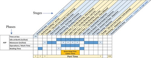
• Arrival port area

• * Towage (Port river located/locks passing)

• Anchoring/Drifting

• Pilot Onboard—Vessel ready to enter

• Vessel Mooring—First rope at entrance

• Pilot Leaving—Boarding at entrance

• Ganga Labor Time

• * On-Site-Shunting—Pilot Onboard

• * On-Site-Shunting—Last Line

• * On-Site-Shunting—First Line

• * On-Site-Shunting—Pilot Offboard

* - Optional stages, depend on weather and port authority pier allocation schedule and priority

• Pilot Order—Vessel ready to departure

• Pilot Onboard—Vessel ready to departure

• Undocking—Unmoor last rope—departure

• Pilot Leaving—departure

• * Towage (Port river located/locks passing)

• ** Vessel Out of Port Area

* - Optional

** - Depend on port policy.

The race for improved efficiency is the basis for almost each stage event of the vessel’s port calling journey, as can be seen in Figure 1.

The main phases of the vessel voyage when calling at port, as described above, are:

• Time at Sea: Sailing time in the country’s territorial zone (port area related), depending on vessel’s assigned schedule.

• Maneuvering time: Actual time vessel is present in the maneuver stage in order to reach berth/shunting/anchorage or departure out.

• Idle time at Berth: Intervals when vessel is present at port piers.

• Operations/Work Time: Actual time when gang operation (cargo handling) starts and ends (i.e. - from end of pilot leaving stage until pilot order—vessel ready for departure).

• Waiting time: The actual time from arrival at the port area and waiting for the start of the maneuver/towage operation and/or when vessel is waiting to start gang labor operation (cargo handling) and/or where gang operation has finished and vessel is ready for departure, waiting to unmoor the last rope and the arrival of the pilot and tug master’s boats.

2.2. Gaps in knowledge

When the vessel calls at a port (or port area), there are two main scenarios for this journey: (A) Calling port for cargo operations (i.e. loading/unloading) and/or (B) Calling port for anchorage reasons (usually for temporary anchorage). From the port perspective, only the first scenario is counted for port time performance and receive the above-mentioned stages that are limited to time efficiency and throughput performance measurement index as this occurs only when the vessel’s temporary schedule work plan is validated. This study hypothesises that the current port time perspective on the examined scenarios and stages has a crucial and significant gap in knowledge, which is significantly important for public and policy decision makers. This study claims that in terms of port emission inventory, the port and port-related area should be looked at in a more comprehensive way. It should include entery/exit country territorial zone stages, which hold both of the internal stages ‘stand by engine’ and ‘full away’ that the vessel goes through in preparation for the port call journey (cargo and/or anchorage). Accordingly, for better understanding of the port contribution to the emissions level arising from the vessels’ presence in port and port-related area (e.g. if for a port cargo call or if for port anchor reasons) these stages must also be considered. Therefore, from the social perspective (i.e. air quality and health) the first and second scenarios as well as additional stages should be counted to assess the vessel’s real ‘Gross Port Time’.

The first scenario: port calling for loading and/or unloading operation (cargo, people, etc.) will now comprise six phases and potentially 21 stages for the port calling journey (compared to the previous phases and 16 potential stages).

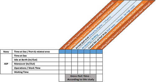
The second scenario: port calling for anchorage reasons will comprise one main phase and seven stages.

These additional stages are important to understand the emission level arising from the vessel’s presence at port and port-related areas (i.e. outside the port area but close to the port perimeter), Since these stages are currently absent from today’s port performance terminology and public discussion, they do not serve as any time performance and/or efficiency index measurement according to port authorities.

These stages of the two main scenarios as illustrated in Figures 2 and 3 include internal stages, described as follows:

Figure 2. First Scenario: Gross Port Time - Vessel Port Calling Journey for Cargo Operation.

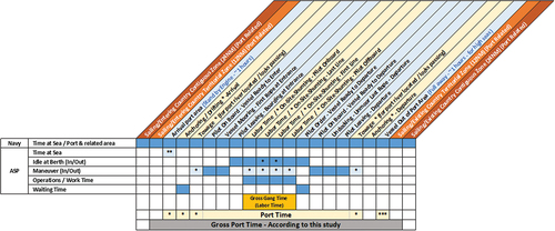
Figure 3. Second Scenario: Vessel Port Calling Journey for Anchorage Reason.

Source: Own composition, based on Israel Navy observation and stages analysis.

Note: Anchoring/Drifting—Time intervals in this scenario may vary between the different types of vessels depending on seasons and vessel owner’s strategy decisions.

Sailing/Entering and Exiting country’s contiguous (24 Nautical Mile - NM) and territorial (12 NM) zone stages. This is usually port geographical position-related, as the vessel can enter the contiguous and territorial zone from different locations with or without a relation to the port area in discussion (e.g. entering contiguous zone from southern Israeli waters, while the sailing destination is Haifa port). Therefore, only the vessel’s geographic location upon entering the territorial zone with relation to speed and distance from the port area was considered.

Stand by engine stage. This usually occurs 5 to 10 nautical miles (NM—around one hour) before the arrival at the designated port area. This stage includes speed reduction operations while the vessel is still at sea, in order to prepare the vessel’s crew and cargo for a full stop (anchorage/drifting) safely upon arrival.

Full away stage. This usually occurs after the vessel is out of the port’s operational area after the pilot vessel’s departure from the vessel’s bridge, around one hour from the port location (i.e. for ocean port location), otherwise depending on the accompanying journey length of the pilot vessel in the exit stage—e.g. river port location). It includes a speed increasing operation, to prepare the vessel’s crew and cargo for full away speed journey safely to the next port.

Anchoring * - Departure stage. This is an optional stage, that usually occurs after the pilot has left the vessel’s bridge. Or it could be due to a maintenance and/or economic reasons (e.g. ahead of next port schedule and/or personal crew issues, maintenance operation that can be only done in the open sea, etc.); or if the vessel company prefers to stay on the open sea (i.e. port related); instead of staying at berth after the gang work has been concluded because of additional expenses for each additional hour of stay.

To summarize, the additional stages are:

• Sailing/Entering Country Contiguous Zone (24 NM) (Port geographical position-related)

• Sailing/Entering Country Territorial Zone (12 NM) (Port geographical position-related)

• Arrival port area (Stand by engine - ~1 hours)

• Anchoring * - Departure

• Vessel Out of Port Area (Full away - ~1 hours—high seas location)

• Sailing/Existing Country Territorial Zone (12 NM) (Port geographical position-related)

• Sailing/Existing Country Contiguous Zone (24 NM) (Port geographical position- related)

2.2.1. “Lost Time” at Port

As reviewed earlier, emission levels arising from a vessel’s presence at port and in the port-related area (i.e. anchorage circles located outside port area but under the port jurisdiction area) are important in scale but are absent from today’s port performance terminology and public discussion. The deviation in time between ASP and Navy the perspective can be considered as ‘Lost Time’ (interval time gaps between temporary and valid schedule work).

Port authorities (private and public) prefer to refer to ‘time at port’ only when the vessel receives a ‘valid’ schedule work plan, assigned with date, pilots shift, designated terminal and pier, working labor shift (gang labor), cranes, etc. Since there are situations where vessel arrives ahead of time and/or a vessel arrives for anchorage reasons (e.g. temporally out of cargo or cargo buyers or vessel Beneficial Cargo Ownership (BCO) looking to maximize its arbitrage potential, etc.) a temporary ‘work invention,’ with a scheduled work plan, is issued by port authorities. This allows the vessel to qualify for a written request for entrance ‘clearance’ check and after Navy inspection is completed a ‘green light’ is given to enter the country territorial waters and port territorial waters area (i.e. anchorage circles) without harming port operation efficiency performance or an increase in its ‘waiting time’ performance.

2.3. The study structure

The following sections present the model description and the following subsections: The methodology section reviews the theoretical and technical background and lays the foundation for the Port and Shoreline Emission Inventory emission inventory model. The description of study analysis procedure section describes the uses of the model input data and explains specific key variables and assumptions used for model. The last section concludes with a summary review, and discussion for strength of the model.

3. Methodology - port and shoreline emission inventory

This chapter develops a generic full bottom-up model framework that looks at the single vessel daily voyage through its port call stages, combined with vessel-specific technical data (such as vessel category type, class, and main/auxiliary engine characteristics, type, speed rate, and Tier grade).and presents its contributionto this research in the maritime transportation field.

3.1. Methodology - Overview

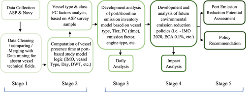
The generic daily port and shoreline emission inventory model framework study methodology is based on full bottom-up approach. The full bottom-up approach (Figure 4) in emission inventory estimation examines the single vessel voyage’s fuel consumption allocation information combined with vessel fleet technical data per vessel (i.e. per IMO number, Vessel Type category, Class, Tier, Deadweight tonnage—DWT and/or Twenty Equivalent Unit—TEU, Length Overall—LOA, etc.). The primary source of this data is based on Navy and ASP records. The output analysis received, after validation and matching process, provides total fuel consumption in port and port related area per vessel visit in minutes (i.e. duration of stay). It is then computed into the individual vessel emission inventory level, providing an analysis tool for estimating the individual vessel emission contribution to the overall emission level in port area and surrounding habitat communities. This represents a piece of the puzzle of air pollutant sources in the port area. The single vessel voyage, based on Navy and ASP observation records, with fuel consumption allocation information per vessel type/class, is adapted from the APS observation survey. The estimated result is then aggregated by vessel category type and vessel class for each of the years observed. This provides figures for the overall emission level arising from aggregate vessel activity in the investigated port and port related area per day, month and year observation analysis.

Figure 4. Overview Description of the Port/Shorline Dailly Emissiom Inventory Study Methodology.

3.2. Description of Study Analysis Procedure

The primary source of data for this study is based on Israel’s Navy and ASP records. Both entities (Navy and ASP) collect information regarding vessel calls for different stages/events of the voyage during a vessel’s presence in Israel’s territorial waters and/or in the port perimeter. This procedure is common and not different from other maritime ports outside of Israel, since all ports and countries worldwide follow IMO international conventions such as ISPS code,² SOLAS,³ FAL⁴ etc.

3.2.1. Computation Vessel Presence Time at Port

Each dataset (Navy and ASP) was loaded to the ‘MYSQL Workbench 8.0 CE Server’ program, creating a table of origin dataset for the investigated period per entity source. Each dataset in its raw form was found to contain multiple and duplicate rows of records per vessel visits. These multiple and duplicate records can be explained by the Navy monitoring each movement event in a different ‘Movement ID’ and the ASP procedure to monitor each pier visit and each primary cargo group and enter them into different rows. Nevertheless, each of these entities manage these multiple and duplicate records of visits under the same key—i.e. unique visit number, a non-repeatable number can be used for only one specific visit. This number is different for each piece of data since each entity is managed by its own information according to its needs. Nevertheless, as when using Big-Data methods on separate datasets gathered from different entities that collect ‘same data’ but from different perspective, a comparison and matching procedure is needed to ensure and validate the datasets that have been collected, increasing the strength and credibility of this study. On the basis of these raw datasets received from the Navy and ASP, two new datasets were constructed enabling this study to compute vessel turnaround times in each port (i.e. vessel presence time). These computations were carried out for each vessel (i.e. per specific IMO number) in each port and for each day (in minutes) according to the ASP and Navy raw datasets. This created two new datasets—‘ASP_Res’ and ‘Navy_Res,’ that present vessel turnaround time in each port per visiting vessel (port call and anchorage) for each source of data.

These datasets are based on the logic of joining and combining records for each vessel using three main parameters: unique visit ID, IMO number and date (arrival and departure). Each dataset records for the vessel’s unique visit are the same for the arrival and departure time stamp records description. Therefore, all three parameters were used to create a new primary key id that was used to ensure avoidance of multiple and/or duplicate records for the single vessel visit in each dataset after combining records procedure. These datasets contain a daily log for each day of each vessel’s time presence. This logic is carried out for each port and area in question in this study. The data hierarchy of the observed vessels according to main datasets used in this study is as shown in Figure 4, as the Navy serves as the ‘Watch Dog’ for each vessel entering territorial water zone. As such, each Navy vessel record covers each ASP vessel visits records.

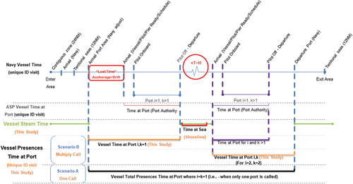
In this study, two main scenarios were considered for computation of the vessel ‘Presence time at port’:

• Scenario A: One port call purpose—i.e. vessel calls at only one port in same territorial area (including anchorage).

• Scenario B: Multiply ports call purpose—i.e. vessel calls at more than one port in same territorial area.

Other scenarios such as an innocent voyage in the territorial waters were not included as they do not appear in the Navy ports visits dataset, as these events are not possible.⁵

3.2.1.1. Scenario A: Call One Port Purpose

The logic behind the computation of the port time procedure for the single vessel visit for the scenario ‘One port call purpose’ is based on vessel port destination, taking into account the vessel’s initial geographic point location with a reference to final destination port (i.e. first observation of vessel’s declared movement towards its final destination port). For example, the scenario describes a simple situation when a vessel calls at only one port under the same Navy registration visit (i.e. same unique ID). The allocated time for $\mathit{port}\left(\mathit{i}=1,\mathit{k}=1\right)$⁶ the single vessel presence visit, includes the interval time between ‘Arrival Port Area—Navy’ (with deduced time factor) and ‘Departure Port Area—Navy’ as described in Figure 5.

Figure 5. Venn Diagram Describing Hierarchy of Observed Vessel According to Main Datasets Used in This Study.

Source: Own composition.

3.2.1.2. Scenario B: Multiply Ports Call Purpose

The logic behind the computation of the port time procedure for the single vessel visit for the scenario ‘Multiple ports call purpose’ describes a situation when a vessel calls at more than one port under same Navy registration visit (i.e. same unique ID within state), with a sailing time T (i.e. steam time) according to the analysis of the average speed and time of observed vessels movements between ports. For example, the scenario describes a simple situation where a vessel calls at more than one port under same unique ID visit. The first port visit $\mathit{port}\left(\mathit{i}=1,\mathit{k}=1\right)$ (k vessel visit numbers under the same Navy registration visit), the allocated time for vessel presence (i.e. ‘time at port’) visit is computed according to the gap interval between ‘Arrival Port Area—Navy’ (with deduced time factor) and ‘Pilot Out—Departure ASP’ based on ASP records. For the second port, the allocated time for $\mathit{port}\left(\mathit{i}=2,\mathit{k}=2\right)$ vessel’s visit presence, including the interval time between ‘Arrival Port Area—ASP’ based on pilot ready or scheduled arrival event and ‘Departure Port Area—Navy’ as described in Figure 5. For areas where a situation of more than two ports of call under the same geographical territorial area is possible under the same Navy unique ID visit (i.e. for countries where $\mathit{port}\left(\mathit{i},\mathit{k}>2\right)$). The allocated vessel presence time for $\mathit{port}\left(\mathit{i},\mathit{k}>2\right)$ can be calculated for the gap interval between ‘Arrival Port Area—ASP’ based on pilot ready or scheduled arrival event and ‘Pilot Out—Departure ASP’ event based on ASP records, similar to that calculated ‘time at port’ according to port authority today. The last port of call i.e. $\mathit{k}>2\mathit{\hspace{0.17em}}\mathit{or}\mathit{\hspace{0.17em}}\mathit{k}=\mathit{k}$, the gap interval for vessel presences time is calculated on ‘Arrival Port Area—ASP’ based on pilot ready or scheduled arrival event and ‘Departure Port Area—Navy’ based on Navy records as describe in Figure 5.

3.2.2. Vessel Fuel Consumption at Port – Israel ASP Survey

The following section presents an analysis of vessel FC at port segmented by category type and class. It is important to state that this analysis can currently be regarded as state of the art, as it is the highest level of FC analysis developed in the maritime transportation literature.

The ASP FC survey is based on observed FC figures that were collected for the overall vessel time at port according to ASP logic of Vessel Presence Time at Port as described in Figure 1. The survey sample is based on a total 108 analyzed records out of 192 observed records. According to the vessel category, all figures have been segmented into different classes of vessels (sub-categories). These figures were collected by the Israel ASP inspection team as each vessel was asked to fill in forms as described in—ASP—MARPOL Annex VI—Survey Template Form, which can be found in (BenHakoun 2020).

The findings of this survey were analyzed per vessel type, class, and total power KW used. These figures were normalized to generate an FC database on a 24-hour visit basis. Findings from the survey analysis as illustrated in Figure 6 show that boiler FC is significant and cannot be overlooked as it today by the IMO in all of its GHG reports. The boiler FC ratio for all OGV were found to be constant to within ~ 30–40% over the entire FC range for 24-Hour port stay (i.e. full day excluding manuvering. The high Boiler FC findings within the Container and Oil Tanker vessel are significantly important as these vessels are known for their high FC performance while at port. Therfore, these findings are sufficiently significant to affect in daily and yearly port emission inventory levels and consequently affect all IMO GHG reports findings (those who preceded the IMO 4^th report).

Figure 6. Time at Port – Vessel Presence Time at Sea/Port - According to Navy, ASP and Study Logic.

Source: Own composition

3.3. Emission inventory equations

To compute and estimate the daily OGVs maritime traffic emission contribution to the local environment, the following emission inventory equations are defined. The following equations are used to estimate the individual vessel emission level while present at port or while sailing along the country’s shoreline.

3.3.1. Port Emission Inventory

In general, the computation and estimation procedures of OGVs’ daily maritime traffic for port emission inventory, depend on three main parameters; FC, Time (T) and Emission Factors (EF). This conclusion is correct if the investigated port is seacoast situated and/or within rivers/lake situated. This procedure can be described in a simplified port emission model framework as shown in Equation 1.(1) $E_{\mathit{\hspace{0.17em}}\left[\mathit{Kg}\right]}=\sum _A\mathit{\hspace{0.17em}}\mathit{FC}\mathit{\hspace{0.17em}}\times \mathit{\hspace{0.17em}}\mathit{T}\mathit{\hspace{0.17em}}\times \mathit{\hspace{0.17em}}\mathit{EF}$(1)

(1) $E_{\mathit{\hspace{0.17em}}\left[\mathit{Kg}\right]}=\sum _A\mathit{\hspace{0.17em}}\mathit{FC}\mathit{\hspace{0.17em}}\times \mathit{\hspace{0.17em}}\mathit{T}\mathit{\hspace{0.17em}}\times \mathit{\hspace{0.17em}}\mathit{EF}$(1)

Where, the FC parameter depends on vessel category type and class, in each activity mode ([MT/min]). Time parameter represents cumulative activity duration per day ([min]), and the EF parameter depends on the vessel’s technical characteristics, i.e. fuel type in use, vessel type and engine (ME, AE) type and grades, etc. ([Kg/MT]).

This general procedure oversimplifies the complexity of the port emission model framework, and as such, the following sections will describe in detail the emission inventory equations. First, starting with defining $E_{i,j}^{P,D}$ equation which is the total Emissions emitted by Vessel (i) of pollutant ($\mathit{j}$) in Day D at port P ($\mathit{P}\ge 1$) (Kilogram [Kg]) as described in Equation 2.(2) $E_{i,j}^{P,D}=\mathit{DVP}{P}_{i,A}^{P,D}\left(\mathit{United}\left|\mathit{ASP},\mathit{Navy}\right.\right)\cdot \mathit{TF}{C}_{i,k,A}^{P,D}\cdot \mathit{E}{F}_{\mathit{i},\mathit{m},\mathit{n},\mathit{k},\mathit{A}}$(2)

(2) $E_{i,j}^{P,D}=\mathit{DVP}{P}_{i,A}^{P,D}\left(\mathit{United}\left|\mathit{ASP},\mathit{Navy}\right.\right)\cdot \mathit{TF}{C}_{i,k,A}^{P,D}\cdot \mathit{E}{F}_{\mathit{i},\mathit{m},\mathit{n},\mathit{k},\mathit{A}}$(2)

The first part of the equation contains the function $\mathit{DVP}{P}_{i,A}^{P,D}$, which describes the Duration of Vessel (i) Port Presence time in Day D at port P ($\mathit{P}\ge 1$) in Activity mode A. This is done according to the study model logic—i.e. United dataset (minutes [min]). The activity mode A was considered for two main mode of vessel operation while at port; Maneuvering and/or Hotelling (i.e. dwell time, berth, anchorage). For each activity mode, the FC depends on the vessel`s technical characteristics as each category and class contain different FC figures. The figures were normalized to 24 hours after deep analysis of the ASP`s vessel FC survey and additional FC sources. Each activity mode FC incorporates engines (ME, AE) and boiler consumption for all port stages.

The second part of the equation contains the function $\mathit{TF}{C}_{i,k,A}^{P,D}$, which is used to describe the Total Fuel Consumed (fuel type k—vector of fuel type; i.e. HFO, MGO, VLSFO⁷ etc.) of Vessel (i) in Day D at port P in Activity mode A as shown in Equation 3.(3) $\mathit{TF}{C}_{i,k,A}^{P,D}\left(\mathit{M}{E}_k,\mathit{A}{E}_k,\mathit{Boile}{r}_k\left|\mathit{ER},\mathit{VT}{C}_i\right.\right)$(3)

(3) $\mathit{TF}{C}_{i,k,A}^{P,D}\left(\mathit{M}{E}_k,\mathit{A}{E}_k,\mathit{Boile}{r}_k\left|\mathit{ER},\mathit{VT}{C}_i\right.\right)$(3)

In simple terms the TFC is the sum factor of ME and/or AE and/or boiler FC (each with fuel type k—nonhomogeneous allowed) in different activity modes (Metric Ton per minute [MT/min]) based on vessel type category and class FC at port analysis. Furthermore, the TFC function based has different characteristics such as: Emission Regulation (ER), Vessel Type and Class (VTC) as described in Equation 4(4) $\mathit{ER}=\left(\mathit{SC},\mathit{\hspace{0.17em}}\mathit{NOx},\mathit{\hspace{0.17em}}\mathit{SCC}\mathit{\hspace{0.17em}}\left(1,0\right)\right)$(4) and 5(5) $\mathit{VT}{C}_i=\mathit{TC}\left(\mathit{IM}{O}_{\mathit{number}},\mathit{SCC}(1,0)\left|\mathit{SizeF}\left(\left.\mathit{IM}{O}_{\mathit{number}}\left|\mathit{VT}\mathit{\hspace{0.17em}}\mathit{Measure}\right.\right|\mathit{LOA},\mathit{BEAM}\left|\mathit{Estimated}\left(1,0\right)\right.\right)\right.\right)$(5) .

(4) $\mathit{ER}=\left(\mathit{SC},\mathit{\hspace{0.17em}}\mathit{NOx},\mathit{\hspace{0.17em}}\mathit{SCC}\mathit{\hspace{0.17em}}\left(1,0\right)\right)$(4)

(5) $\mathit{VT}{C}_i=\mathit{TC}\left(\mathit{IM}{O}_{\mathit{number}},\mathit{SCC}(1,0)\left|\mathit{SizeF}\left(\left.\mathit{IM}{O}_{\mathit{number}}\left|\mathit{VT}\mathit{\hspace{0.17em}}\mathit{Measure}\right.\right|\mathit{LOA},\mathit{BEAM}\left|\mathit{Estimated}\left(1,0\right)\right.\right)\right.\right)$(5)

The ER parameter defines a function that checks the existence of local and/or regional and/or global regulation regarding the following subjects: limitation of fuel Sulfur Content (SC), NOx limits and Shore Connection Capabilities (SCC—can also be refer as Alternative Marine Power—AMP) availability that match the technical requirements of port (piers) and vessel (Y/N). This returns correct indicators to ensure correct fuel type and EF assignments per each vessel (i).

The VTC function defines a Vessel Type and Class (TC) that check and determine vessel type category, vessel classification size group and indication of SCC. This function is based on inputs received from the vessel fleet dataset, for each IMO number and vessel’s actual size according to the Size Function (SizeF) return parameter. The SizeF defines the Size Function, which investigates and is validated per IMO number vessel type category and class size.

The third part of the equation contains the EF function, which is used to determine and allocate EF for each vessel (i) with engine type (m) and designed engine speed grade (n) that consumed Fuel Type (k) per mode of activity (A) while at port (P), with reference to vessel category type and class. The function returns EF based on different function parameters such as engine type and speed grade (for AE and ME), Fuel Type (FT), vessel engine Tier grade while taking current Emission Regulation (ER) into consideration, as described in Equation 6.(6) $\mathit{E}{F}_{\mathit{i},\mathit{m},\mathit{n},\mathit{k},\mathit{A}}(\mathit{Engin}{e}_{\mathit{i},\mathit{m},\mathit{n}},\mathit{F}{T}_{k,m,n,A}^P,\mathit{Tie}{r}_{\mathit{i},\mathit{l}}\left|\mathit{ER}\right.)$(6) The Emission unit is defined as Gram to Kilogram of fuel consumption [g/Kg fuel].

(6) $\mathit{E}{F}_{\mathit{i},\mathit{m},\mathit{n},\mathit{k},\mathit{A}}(\mathit{Engin}{e}_{\mathit{i},\mathit{m},\mathit{n}},\mathit{F}{T}_{k,m,n,A}^P,\mathit{Tie}{r}_{\mathit{i},\mathit{l}}\left|\mathit{ER}\right.)$(6)

As some vessels have different configurations of ME (i.e. SSD, MSD or HSD⁸) that may affect the primary fuel in use, this may affect FT in use in AE and boiler. The function returns an indication regarding engine type (m) and designed engine speed grade (n) with reference to vessel category type and class is described in Equation 7.(7) $\mathit{Engin}{e}_{\mathit{i},\mathit{m},\mathit{n}}=\left\{\begin{array}{cc}1& 2-\mathit{Stroke}\\ 0& 4-\mathit{Stroke}\end{array}\mathit{\hspace{0.17em}}\left|\mathit{\hspace{0.17em}}\begin{array}{c}1\\ 2\\ 3\end{array}\mathit{\hspace{0.17em}}\begin{array}{c}\mathit{SSD}\\ \mathit{MSD}\\ \mathit{HSD}\end{array}\right.\right.$(7)

(7) $\mathit{Engin}{e}_{\mathit{i},\mathit{m},\mathit{n}}=\left\{\begin{array}{cc}1& 2-\mathit{Stroke}\\ 0& 4-\mathit{Stroke}\end{array}\mathit{\hspace{0.17em}}\left|\mathit{\hspace{0.17em}}\begin{array}{c}1\\ 2\\ 3\end{array}\mathit{\hspace{0.17em}}\begin{array}{c}\mathit{SSD}\\ \mathit{MSD}\\ \mathit{HSD}\end{array}\right.\right.$(7)

The Fuel Type (FT) function defines and returns one of the two main fuel type class categories (k) in use per each engine type (m) and designed engine speed grade (n) per mode of activity (A) while at port (P). The categories are Residual Marine (RM) and Distillates Marine (DM), Other (LNG, Ammonia, Methanol, etc.) each with a different per cent of SC depend on existing ER requirements and/or emission reduction equipment installed onboard, as described in Equation 8.(8) $\mathit{F}{T}_{k,A}^P\left(\mathit{VesslType}\right)=\left\{\begin{array}{ccc}2& \mathit{\hspace{0.17em}}& \mathit{Other}\mathit{\hspace{0.17em}}(\%\mathit{SC}\left|\mathit{ER}\right.)\\ 1& \mathit{\hspace{0.17em}}& \mathit{RM}\mathit{\hspace{0.17em}}(\%\mathit{SC}\left|\mathit{ER}\right.)\\ 0& \mathit{\hspace{0.17em}}& \mathit{DM}\mathit{\hspace{0.17em}}(\%\mathit{SC}\left|\mathit{ER}\right.)\end{array}\right.$(8)

(8) $\mathit{F}{T}_{k,A}^P\left(\mathit{VesslType}\right)=\left\{\begin{array}{ccc}2& \mathit{\hspace{0.17em}}& \mathit{Other}\mathit{\hspace{0.17em}}(\%\mathit{SC}\left|\mathit{ER}\right.)\\ 1& \mathit{\hspace{0.17em}}& \mathit{RM}\mathit{\hspace{0.17em}}(\%\mathit{SC}\left|\mathit{ER}\right.)\\ 0& \mathit{\hspace{0.17em}}& \mathit{DM}\mathit{\hspace{0.17em}}(\%\mathit{SC}\left|\mathit{ER}\right.)\end{array}\right.$(8)

The Tier level (l) ($\mathit{Tie}{r}_l$) function classifies and validates each IMO number according to its year-built information, TechEmission technologies installed, and ER in force at the local level as described in Equation 9.(9) $\mathit{Tie}{r}_{\mathit{i},\mathit{l}}\left(\mathit{IM}{O}_{\mathit{number}}\left|\mathit{BuildYear}\left|\mathit{TechEmission}\left(\mathit{ER}\right)\right.\right.\right)=\left\{\begin{array}{cc}0& \mathit{Before}\mathit{\hspace{0.17em}}2000\\ 1& 2000-2010\\ 2& 2011-2015\\ 3& 2016\mathit{\hspace{0.17em}}\mathit{and}\mathit{\hspace{0.17em}}\mathit{above}/\mathit{ER}\end{array}\right.$(9) This determines NOx EF limits for each engine type (m) and designed engine speed grade (n) Tier level, based on IMO, MARPOL Annex VI, Reg. 13 classification and NOx TechEmission technologies installed. NOx reduction technologies such as Selective Catalytic Reduction (SCR), Exhaust Gas Recirculation (EGR), Dual Fuel engine (DF—combination of LNG and fuel oil).

Tier III SSD engines currently present a range reduction of 76% to 80% of NOx compared to Tier II and I respectively (Winnes et al. 2016). Yet, they need to be operated manually to achieve this reduction (i.e. Tier III vessels out of NOx ECA, are considered Tier II vessels). Therefore, local Emission Regulation (ER), can also determine operate mode of emission reduction technologies such as Selective Catalytic Reduction (SCR), Exhaust Gas Recirculation (EGR), Dual Fuel engine (DF—combination of LNG and fuel oil), etc., that enable the reduction of NOx.

(9) $\mathit{Tie}{r}_{\mathit{i},\mathit{l}}\left(\mathit{IM}{O}_{\mathit{number}}\left|\mathit{BuildYear}\left|\mathit{TechEmission}\left(\mathit{ER}\right)\right.\right.\right)=\left\{\begin{array}{cc}0& \mathit{Before}\mathit{\hspace{0.17em}}2000\\ 1& 2000-2010\\ 2& 2011-2015\\ 3& 2016\mathit{\hspace{0.17em}}\mathit{and}\mathit{\hspace{0.17em}}\mathit{above}/\mathit{ER}\end{array}\right.$(9)

3.3.2. Shoreline Emission Inventory

This section will describe the Shoreline Emission Inventory equations., Although it is constructed for all vessel type categories and classification size group compatibility, in this study it will be used only for container vessels.

First, starting with defining $E_{i,j}^{Z,D}$ equation which is the total Emissions emitted by Vessel (i) of pollutant ($\mathit{j}$) in Day D at Zone Z ($\mathit{Z}\ge 1$) (Kilogram [Kg]) as describe in Equation 10.(10) $E_{i,j}^{Z,D}=\mathit{DVS}{T}_i^{Z,D}\cdot \mathit{TF}{C}_{i,k}^{Z,D}\cdot \mathit{E}{F}_{\mathit{i},\mathit{m},\mathit{n},\mathit{k},\mathit{A}}$(10)

(10) $E_{i,j}^{Z,D}=\mathit{DVS}{T}_i^{Z,D}\cdot \mathit{TF}{C}_{i,k}^{Z,D}\cdot \mathit{E}{F}_{\mathit{i},\mathit{m},\mathit{n},\mathit{k},\mathit{A}}$(10)

The first part of the equation contains the function $\mathit{DVS}{T}_i^{A,D}$, that describes the minimum Duration of Vessel (i) Steam Time between Port to Port (P2P), a comparison between average length of voyage (NM) divided by average speed (Kn/min) compared to Vessel (i) Steam Time according to United dataset model logic (minutes [min]) as describe in Equation 11.(11) $\mathit{DVS}{T}_i^{Z,D}\left(\mathit{Mi}{n}_{\mathit{Steam}\mathit{\hspace{0.17em}}T\mathrm{ime}}\left[\left(\mathit{Length}/\mathit{Kn}\right),\left(\mathit{United}\left|\mathit{ASP},\mathit{Navy}\right.\right)\right]\right)$(11)

(11) $\mathit{DVS}{T}_i^{Z,D}\left(\mathit{Mi}{n}_{\mathit{Steam}\mathit{\hspace{0.17em}}T\mathrm{ime}}\left[\left(\mathit{Length}/\mathit{Kn}\right),\left(\mathit{United}\left|\mathit{ASP},\mathit{Navy}\right.\right)\right]\right)$(11)

The second part of the equation contains the function $\mathit{TF}{C}_{i,k}^{Z,D}$, which describes the Total Fuel Consumption of vessel (i) in Day (D) and at Zone Z for fuel type (k) as described in 12. Where, TFC is the sum factor of FC performance per speed (knots) and duration (min) based on cardinal sail directions and average steam time (according to observations based on this study’s logic model). The FC figures are based primarily on ME combined with AE and boiler FC figures based on data received from major international shipping companies in the liner sector (Metric Ton per minute [MT/min]). Where TFC function based on different characteristics such as ER and VTC as described in Equation 4(4) $\mathit{ER}=\left(\mathit{SC},\mathit{\hspace{0.17em}}\mathit{NOx},\mathit{\hspace{0.17em}}\mathit{SCC}\mathit{\hspace{0.17em}}\left(1,0\right)\right)$(4) and 5(5) $\mathit{VT}{C}_i=\mathit{TC}\left(\mathit{IM}{O}_{\mathit{number}},\mathit{SCC}(1,0)\left|\mathit{SizeF}\left(\left.\mathit{IM}{O}_{\mathit{number}}\left|\mathit{VT}\mathit{\hspace{0.17em}}\mathit{Measure}\right.\right|\mathit{LOA},\mathit{BEAM}\left|\mathit{Estimated}\left(1,0\right)\right.\right)\right.\right)$(5) in the Port Emission Inventory model framework above.

(12) $\mathit{TF}{C}_{i,k}^{Z,D}\left(\mathit{M}{E}_k(\mathit{Kn}\left|\mathit{CardinalDirection},\mathit{\hspace{0.17em}}\mathit{SteamTim}{e}_{\mathit{Avg}}\right.),\mathit{A}{E}_k,\mathit{Boile}{r}_k\left|\mathit{ER},\mathit{VT}{C}_i\right.\right)$(12)

The third part of the equation contains the EF function, which is used to determine and allocate EF for each vessel (i) with engine type (m) and design engine speed grade (n), sharing the same function parameters as described in Equation 6(6) $\mathit{E}{F}_{\mathit{i},\mathit{m},\mathit{n},\mathit{k},\mathit{A}}(\mathit{Engin}{e}_{\mathit{i},\mathit{m},\mathit{n}},\mathit{F}{T}_{k,m,n,A}^P,\mathit{Tie}{r}_{\mathit{i},\mathit{l}}\left|\mathit{ER}\right.)$(6) , 7(7) $\mathit{Engin}{e}_{\mathit{i},\mathit{m},\mathit{n}}=\left\{\begin{array}{cc}1& 2-\mathit{Stroke}\\ 0& 4-\mathit{Stroke}\end{array}\mathit{\hspace{0.17em}}\left|\mathit{\hspace{0.17em}}\begin{array}{c}1\\ 2\\ 3\end{array}\mathit{\hspace{0.17em}}\begin{array}{c}\mathit{SSD}\\ \mathit{MSD}\\ \mathit{HSD}\end{array}\right.\right.$(7) , 8(8) $\mathit{F}{T}_{k,A}^P\left(\mathit{VesslType}\right)=\left\{\begin{array}{ccc}2& \mathit{\hspace{0.17em}}& \mathit{Other}\mathit{\hspace{0.17em}}(\%\mathit{SC}\left|\mathit{ER}\right.)\\ 1& \mathit{\hspace{0.17em}}& \mathit{RM}\mathit{\hspace{0.17em}}(\%\mathit{SC}\left|\mathit{ER}\right.)\\ 0& \mathit{\hspace{0.17em}}& \mathit{DM}\mathit{\hspace{0.17em}}(\%\mathit{SC}\left|\mathit{ER}\right.)\end{array}\right.$(8) and 9(9) $\mathit{Tie}{r}_{\mathit{i},\mathit{l}}\left(\mathit{IM}{O}_{\mathit{number}}\left|\mathit{BuildYear}\left|\mathit{TechEmission}\left(\mathit{ER}\right)\right.\right.\right)=\left\{\begin{array}{cc}0& \mathit{Before}\mathit{\hspace{0.17em}}2000\\ 1& 2000-2010\\ 2& 2011-2015\\ 3& 2016\mathit{\hspace{0.17em}}\mathit{and}\mathit{\hspace{0.17em}}\mathit{above}/\mathit{ER}\end{array}\right.$(9) in the Port Emission Inventory model framework above. The equations developed in the Port Emission Inventory model framework and in the Shoreline Emission Inventory model framework are used to answer the research questions.

In order to answer the research questions regarding what the port emission inventory for GHG and CACs emissions and who are the main OGVs pollutant emitters contributors in the port area (per vessel category type and class) and what is the contribution of each stage/mode of operation, the following equations will be developed.

For Port Emission Inventory ($\mathit{PortEI}$) for investigated port (P) and emission type (j) for one-year period Equation 13(13) $\mathit{PortE}{I}_j^P=\sum _{\mathit{i}=1}^n\sum _{\mathit{D}=1}^{365}{E}_{i,j}^{P,D}$(13) , was developed:

(13) $\mathit{PortE}{I}_j^P=\sum _{\mathit{i}=1}^n\sum _{\mathit{D}=1}^{365}{E}_{i,j}^{P,D}$(13)

For Shoreline Emission Inventory ($\mathit{ShorelineEI}$) for investigated Zone Z for a one-year period, the following Equation 14(14) $\mathit{ShorelineE}{I}_j^Z=\sum _{\mathit{i}=1}^n\sum _{\mathit{D}=1}^{365}{E}_{i,j}^{Z,D}$(14) , was developed.

(14) $\mathit{ShorelineE}{I}_j^Z=\sum _{\mathit{i}=1}^n\sum _{\mathit{D}=1}^{365}{E}_{i,j}^{Z,D}$(14)

4. Case study - Israel main ports and shoreline

4.1. Case study scope

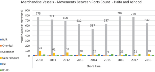
Given the significance of this topic, this paper presents a review case study of daily port and shoreline emission inventory arising from shipping activity operating in same sea area. The main criterion considered when choosing ports (Ashdod and Haifa) was a combination of sea location, ports trade reciprocity, and data availability. The aim of case study is to describe and demonstrate the model capabilities for measurements of the environmental impacts of shipping activity along port cities and shoreline. Findings from the model framework analysis show that the vast majority of vessel movements between Israel’s main ports (within Israel’s 24 NM zone) are done by the liner shipping sector, with an average of 707⁹ annual movements, which can be translated to 14 weekly movements, as shown in Figure 7.

Figure 7. ASP Survey - ME, AE and Boiler - FC by Type and Class (in %).

Source: Own calculation

AE and Boiler FC figures—based on Israel ASP FC at port survey—own analysis (figures collected onboard by ASP inspection team and/or reported by vessel master)

ME FC based on DTU 2016 FC at port analysis for port that is seaside located (i.e. maneuvering duration of 10–15minutes)

FC figures for Passenger/Cruise vessels were provided by a major vessel charter agency specializing in Passenger/Cruise vessels from the Aegean Sea (without classification of ME, AE and Boiler).

All FC figures were validated with major liner shipping company, vessel charter agency and known Capt. in Israel maritime sector.

Due to technical limitations, the category Passengers (cruise) vessels were shortened to PASS.

Reliable FC data for steaming operation per knots and per vessel class was available only for the liner shipping (i.e. Container). Therefore, this case study has included only the liner shipping vessels in its computation procedure for vessel steam time, vessel FC and vessel voyage emission inventory along Israel’s shoreline. According to the above case study guideline, the daily port emission inventory capability in this paper will be demonstrated for liner shipping only. The case study estimates and demonstrate the model capabilities for daily emission inventory of Haifa Port and Ashdod Port and the Israel Shoreline P2P vessel’s movements for the period 2010–2018. The main CACs emissions targeted in this case study are SOx, NOx, CO, HC and PM (SOx, NOx for the port, all CAC for the shoreline model).

Emission factors baselines, SFOC, Fuel Type, Engine spec, SC and other assumptions and information for the Israel daily ports and shoreline shipping case study can be found in BenHakoun (2020).

4.2. Israel Port - Fuel Type in Use

HFO is the most commonly used fuel in Israel ports (pre-2020). This assumption is logical and economically wise for all vessels within ports as Israel does not have a local set of limitations for SC in bunker fuels, since Israel’s current policy is to be in line with IMO global regulation. Yet, to strengthen this assumption, the data samples of the FC survey was analyzed by fuel type for ME, AE and boilers, thereby removing any uncertainty in the model for this issue. As expected, findings show that HFO was the most common fuel in use for OGV vessels within Israeli ports for both ME, AE and boilers alike.

4.2.1. Sailing speed around Israel shoreline

To better answer questions regarding emission inventories levels along Israel shoreline, the sailing speed between P2P was investigated. Findings from the model show that each event where a single vessel calls on more than one port in the same territorial waters in Israel, indicates that this vessel’s journey included movements between ports (Haifa and Ashdod) with a gap of 24 hours or less. Analysis of the average voyage duration time between Israel ports was found to be significantly lower at an average of 6 hours. Another scenario that was considered describes vessel departure/arrival from/in one port and staying at anchorage outside the port area for more than 24 hours and then continuing its journey towards the next port (within Israel) while sailing in the territorial waters. This type of movement is cover under the navy registration movements ID visits. Nevertheless, the data was searched for movements between ports with a time gap greater than 24 hours (i.e. − 36, 48 and 72 hours), but not a single record that matched this movement description was found. As only container vessels have been included in the computation procedure for vessel steam time, FC and emission inventories around Israel shoreline. As each P2P movement was lacking information regarding speed and duration, additional data were needed. Data collected from one of the major shipping companies in the liner sector regarding speed, length and duration of movements between ports, per unique trade lanes was used to investigate speed, distance and steam duration as summarized in Tables 1 and 2. Findings from the analysis indicate variations in speed depend on sail direction, as North to South voyage speed is slower than South to North voyage speed (North to South—i.e. ILHFA to ILASH or South to North—i.e. ILASH to ILHFA).

Table 1. ILASH-ILHFA weighted sample average for sailing speed, steam hours and distance cross.

ILASH-ILHFA (2014–2019. Aug)	Sailing Speed (Kn)	Steam Hours (Hr)	Distance (NM)
Sample Size (No. Passes)	810	810	810
No. of Trade lanes in Sample (unique)	13	13	13
Weighted sample average	14.40	5.57	73.68
Weighted sample variance	0.71	0.44	2.99
Weighted sample standard deviation	0.84	0.66	1.73
Coefficient of variation	5.8%	11.9%	2.3%

Table 2. ILHFA-ILASH weighted sample average for sailing speed, steam hours and distance cross.

ILHFA-ILASH (2014–2019. Aug)	Sailing Speed (Kn)	Steam Hours (Hr)	Distance (NM)
Sample Size (No. Passes)	865	865	865
No. of Trade lanes in Sample (unique)	13	13	13
Weighted sample average	14.1	5.4	73.00
Weighted sample variance	1.62	0.46	1.72
Weighted sample standard deviation	1.27	0.68	1.31
Coefficient of Variation	9.0%	12.5%	1.8%

Source: This study, based on data received from a major shipping company in the liner sector.

This variation for liner shipping, can be explained by two main factors:

1. Vessels sailing from south to north, most likely have crossed the Suez Canal (i.e. returning from Asia) and are loaded with full containers onboard, and as such, supply time is now crucial.

2. Vessels sailing from north to south are not on a tight schedule to catch its reserved slot for passage through the Suez Canal, since it is scheduled to call one last port before reaching the canal.

To provide conservative figures, the lower boundary of a weighted sample average for sailing speed was chosen to describe the average speed (Kn) for liner vessels; movements between Israel ports ILHFA to ILASH—is 14.1 Kn and ILASH to ILHFA—is 14.4 Kn.

4.2.2. Accuracy and Reliability

Vessels movement data and FC data are the pillars of the port and shoreline emission inventory model frameworks. The strength of the first pillar, vessel movement data, relies on the fact that it comes from official sources. The Israeli Navy and the Israeli ASP are two different entities with separate and different methods for collecting and documenting vessel movements within Israel. Nevertheless, the accuracy of the datasets received from the Israel Navy and Israel ASP, is considered extremely high, as both serve as ‘watch dogs’ for maritime movements.

The strength of the second pillar, FC data, relies on the fact that the data comes from an official survey conducted by the ASP Department of Supervision and Control in ports. FC for steam was based on data provided by major liner shipping company. All FC figures in this study were validated by recognized professional sources.

4.3. Israel Shore line

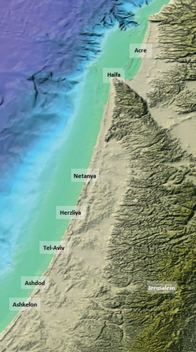
Located on the eastern side of the Mediterranean, Israel shares a long shoreline with known corridor trade lanes that go in and out of the Suez Canal from Turkey, Cyprus, and the Balkan. The majority of Israel’s residential areas and population are concentrated along a narrow strip along the Israel shoreline (as shown in Figure 8).

Figure 8. Merchandise Vessels - Movements Between Ports Count - Haifa and Ashdod - for Years 2010–2018.

Source: Own composition, based on the model logic.

This narrow strip surface can be described as a plateau with dense residential areas, and as such serves as an important area for investigation.

4.3.1. P2P – vessels movements emission inventory (Total)

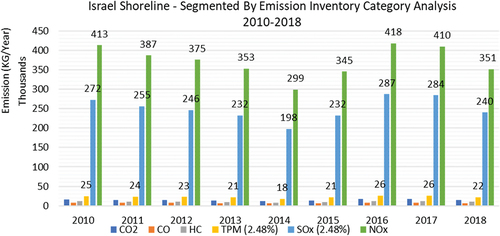
Findings from the model show that the estimated total emission inventory emitted along Israel’s shoreline by container vessels is an average between 345 to 418 tons of NOx and annual average between 232 to 287 tons of SOx. This can be translated to a weekly average of 6.8–8.2 tons of NOx and 4.5–5.6 tons of SOx, as shown in Figure 9.

Figure 9. Israel shoreline - shaded relief map.

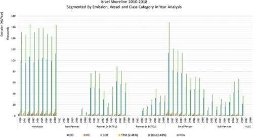
Container vessel movements between two ports that are close to each other (i.e. under the same cluster trade definition) usually occur due to the need to reposition cargo by a logistic balancing operation of empty boxes and to other freight movements such as load and unload of cargo (local and transshipment). From the analysis of nine years of historical vessel movements, voyages and emission inventory performance, the small/feeder container vessels’ contribution to the estimated annual total emission inventory is decreasing. While findings from the model indicate that the contribution of the Panamax (>8K TEU) and Neo Panamax (>12.5K TEU) to the annual estimated total emission inventory have increased significantly, as shown in Figure 10.

Figure 10. Cumulative Emissions at Israel Shoreline by Container Vessels - Segmented by Emission Type in Year Performance Analysis.

The following figures present different aspects of the findings from the Shoreline emission inventory’s calibrated model framework. Aspects such as vessel FC in daily performances, FC ratio distribution in quarter performances and estimated inventory for different types of CAC and GHG emission in daily and quarter performances analyses. All findings are shown in the stacked column chart analysis in order to track trend changes over time and comparing different periods and different vessel class contributions. The horizontal axis shows the performances of different vessel classes in daily, monthly, and/or quarterly and/or yearly analysis level. The vertical axis shows the sum of performances archived. The vertical axis shows different units of measure, from Metric Ton (MT) to percentage ratio, etc.

4.3.2. NOx

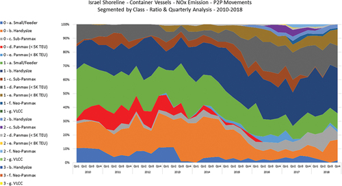
In estimating NOx emissions from P2P vessel movements, this study assumed that vessel age is an important component in defining engine Tier grade. Therefore, this study addressed the selected Tiers: 0, 1, 2, and 3, which serve as indicators for NOx emission standards for SSD, MSD and HSD engines depending on the engine design efficiency for maximum operating speed (n, rpm). Figure 11 shows the shift in class and in Tier engine grade trends. The shift in trends shows a decrease in contribution from vessels from engine grade Tier 0 (i.e. Small/Feeder, Handy Size, Panamax (<5K TEU)) and Tier 1 (i.e. Small/Feeder, Sub- Panamax). In contrast, the trend shifts reveal an increase in the contribution from vessels of engine Tier 0 (i.e. Sub-Panamax), Tier 1 (i.e. Handy Size, Panamax < 5K TEU and Panamax < 8K TEU) and vessels of Tier 2 (i.e. Handy Size, Sub-Panamax and Neo Panamax < 12.5K TEU). Other vessels from Tier 3 engine grade were found to be insignificant in frequency of P2P vessel movements, therefore were insignificant in their contribution. These findings are within normal expectations as the current liner fleet is being renewed worldwide.

Figure 11. Cumulative emissions at israel shoreline by container vessels - segmented by emission type, class category in year performance analysis.

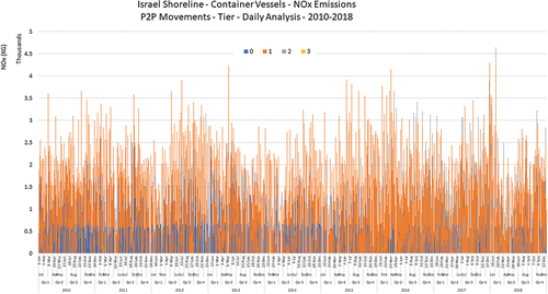
In terms of daily average NOx emission, Container vessels along the Israel shoreline are estimated to be responsible for a daily average of ~ 2–2.5 tons for 2010–2017 and a daily average of ~ 1.6–2 tons for 2017–2018. In terms of Tier grade level analysis, as expected, Tier 1 engine grade vessels are dominant, as shown in Figure 12.

Figure 12. Nox emissions by container vessels across israel shoreline - segmented by engine tier grade, category and class in ratio and quarter analysis.

4.3.3. SOx

In terms of SOx emission, findings from the model, Figure 13 shows that the average daily SOx emissions along the Israel shoreline range between ~ 1 to ~ 1.5 MT for years 2010– 2018. An average increase in trend for the upper boundary to ~ 1.8–2 MT for years 2015–2018 can be seen due to an increase in P2P movements frequency of vessels size 5K TEU and above.

Figure 13. Nox emissions by container vessels across israel shoreline - segmented by engine tier grade, in cumulative daily analysis.

4.4. Israel main ports overviews

Israel seaports are responsible for more than 99% of Israel international trade in terms of export and import and around 80% in terms of value.¹⁰ Israel’s main international trade ports are Haifa and Ashdod and are currently public owned port. Haifa and Ashdod Ports are considered ports that are highly connected to other international maritime transportation trade lanes.

The following sections present the analysis results of the daily Port Emission Inventory Model. To present the total emission contribution of the single vessel voyage while in port and port-related area, it is necessary to include the ME, AE and boiler FC contribution to the analysis. The estimated contribution of the ME requires a complex analysis based on engine power, vessel size, type of vessel and other parameters such as propeller efficiency, numbers of propeller blades, water and air resistance, etc., as mentioned in the Danish model. In addition, other factors that may effect ME FC are needed to be considered; factors such as maneuvering duration (i.e. low sail speed of ~ 4-6 NM in/out anchorage circles/port, stopping operation, anchor lifting, etc. Findings from the analysis indicate that the ME FC contribution to the total port FC, are estimated at ~ 2.6%-4.8% of the total annual port FC (depending on port and year), i.e. the ME FC contribution to the Port Emission Inventory Model are not significant to the model results. Therefore, to present conservative figures, the following analysis sections were based only on AE and Boiler FC performance, as the ME FC figures were not included in the original ASP FC survey.

4.4.1. Haifa - containers shipping emission inventory

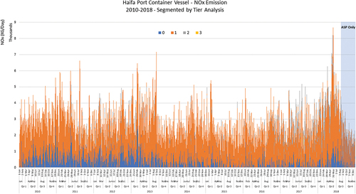
Haifa Port serves as one of the two main significant ports and economic bridge of Israel with the outside world. Haifa Port facilities handled an average annual of ~ 1.26 Million TEU (Export & Import) for the pre-2017 period and for ~ 1.38 Million TEU afterwards, as shown in Figure 14. Haifa Port showed an average annual growth of 2% for all periods. Findings from the Port Emission Inventory Model framework show that Handysize, Panamax (<5K TEU), and Panamax (<8K TEU) classes dominate Haifa Port Container vessel statistics. As illustrated in Figure 15, shifting class trends can clearly be seen from 2016 and afterwards, which show an increase in frequency of call for the Neo-Panamax (<12K TEU) and the VLCS (>14.5K TEU) vessels. Which comes at the cost of frequency of call for Handysize (<2K TEU) and small/feeder (<1K TEU) vessels. In terms of daily average NOx emission, Container vessels in Haifa Port are estimated to be responsible for a daily average of ~ 2–2.7 tons for 2010–2017 and a daily average of ~ 2.6–3.2 tons for 2017–2018. In terms of Tier grade level analysis, as expected, Tier 1 engine grade vessels are dominant, as shown in Figure 16. In term of daily average SOx emission, Containers vessels in Haifa Port are estimated to be responsible for a daily average of ~ 0.2–0.24 tons for 2010–2016 and a daily average of ~ 0.24–0.3 tons for 2017–2018, as shown in Figure 17. This increase in daily emission inventory can be explained by two main reasons: (a) An increase in frequency calls of the Neo-Panamax (<12K TEU) and Very Large Container Ship (VLCS), which carry 12K TEU and above. These vessels are known for their high FC performance while at port. (b) An increase in waiting and operation time (i.e. employee’s sanctions, which started to increase in frequency since the announcement of the port structure reform in 2013 and gradually reached a peak in 2018 as the decision date approached).

Figure 14. SOx Emissions by Container Vessels Across Israel Shoreline - Segmented by Class Category in Daily Performance Analysis.

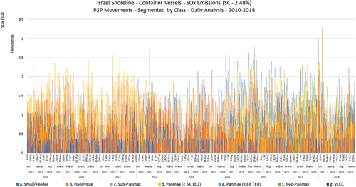
Figure 15. Container Vessels - Total Export & Import (TEU) at Haifa Port - Segmented by Class Category in Year Performance Analysis.

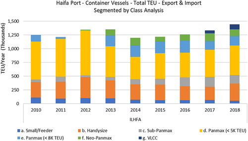
Figure 16. Container Vessels - Visit Count at Haifa Port - Segmented by Class Category in Year Trend Analysis.

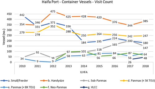
Figure 17. NOx Emissions by Container Vessels at Haifa Port - Segmented by Engine Tier Grade in Daily Performance Analysis.

Additional findings indicate that upon arrival to the port jurisdiction areas, vessels above 8K TEU were very frequently found to be responsible for half of the daily total port emissions in comparison to the total existing OGV fleet in Haifa Port at that day. This analysis would be subject to change if each vessel’s operational reefers (i.e. refrigerated containers) onboards were to be incorporated in this analysis (as they are expected to increase vessel FC).

4.4.2. Ashdod - Containers Shipping Emission Inventory

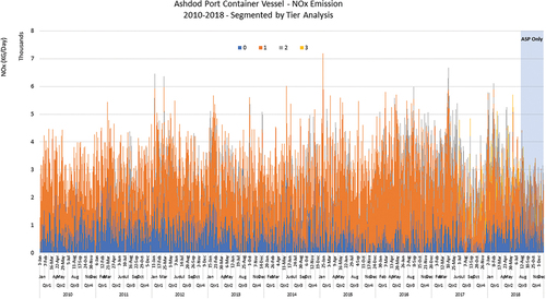
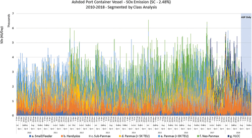
Ashdod Port facilities handled an average annual of ~ 1.16 Million TEU (Export & Import) for the pre-2016 period and for ~ 1.4 Million TEU afterwards, as shown in Figure 18. Despite a decline in the total annual throughput in 2014–2015 and 2018, Ashdod Port showed an average annual growth of ~ 3.4% for all periods. Findings from the Port Emission Inventory Model framework show that the Handysize, Panamax (<5K TEU), Panamax (<8K TEU), and Neo-Panamax (<12K TEU) classes dominate Ashdod Port Container vessel statistics. As illustrated in Figure 19, shifting class trends can clearly be seen from 2012 and afterwards, which show an increase in frequency of call for the Neo-Panamax (<12K TEU) which carries 8K TEU and above and from 2017 the VLCS (>14.5K TEU) vessels. This comes at the cost of frequency of call for the small/feeder (<1K TEU) and the Panamax (which carry from 5K TEU to 8K TEU) vessels. In terms of daily average NOx emission, Container vessels in Ashdod Ports are estimated to be responsible for a daily average of 2.6–2.8 tons for 2010–2017 and a daily average of 3.1–3.6 tons for 2017–2018. In terms of Tier grade level analysis, as expected, with Tier 1 engine grade are dominant, as shown in Figure 20. In terms of daily average SOx emission, Containers vessels in Ashdod Port are estimated to be responsible for a daily average of 2.4–2.7 tons for 2010–2016 and a daily average of 2.9–3.4 tons for 2017–2018, as shown in Figure 21. This increase in daily emission inventory can be explained by two main reasons: (a) An increase in call frequency of the Sub-Panamax (<3K TEU), Neo-Panamax (<12K TEU) and VLCS (>14K TEU). These vessels are known for their high FC performance while at port. (b) An increase in waiting and operation time (i.e. employee’s sanctions,).

Figure 18. SOx Emissions by Container Vessels at Haifa Port - Segmented by Class Category in Daily Performance Analysis.

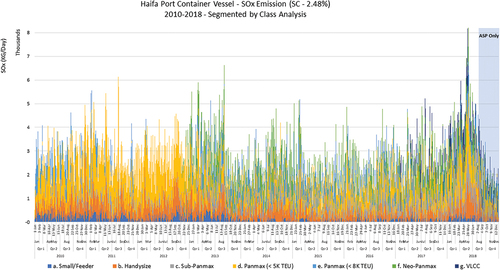
Figure 19. Container Vessels - Total Export & Import (TEU) at Ashdod Port - Segmented by Class Category in Year Performance Analysis.

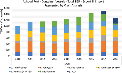
Figure 20. Container Vessels - Visit Count at Ashdod Port - Segmented by Class Category in Year Performance Analysis.

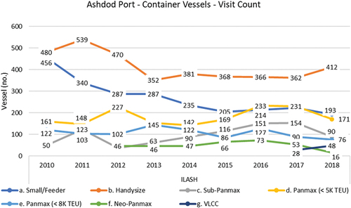
Figure 21. NOx Emissions by Container Vessels at Ashdod Port - Segmented by Engine Tier Grade in Daily Performance Analysis.

Additional findings indicate that upon arrival to the port jurisdiction areas, vessels above 8K TEU were very frequently found to be responsible for half of the daily total port emissions in comparison to the total existing OGV fleet in Ashdod Port at that day as shown in Figure 22. This is similar to Haifa Port, but with an even higher magnitude. This analysis would be subject to change if each vessel’s operational reefers (i.e. refrigerated containers) onboards were to be incorporated in this analysis.

Figure 22. SOx Emissions by Container Vessels at Ashdod Port - Segmented by Class Category in Daily Performance Analysis.

5. Discussion

International shipping is one of the key components in our world economy and has a significant role in the ‘globalization’ effort. Today as environmental awareness is increasing worldwide, there has been an increased concern for environmental issues related to the global supply chain (UNCTAD, United Nations Conference on Trade and Development 2018). The worldwide awareness for shipping and port environmental effects has led to an increase in academic case studies of ports’ emissions effect on residential areas in the last decades. Many of these studies are based on activity-based methods, either by the top-down approach or by the full bottom-up approach. The majority of these studies based their analyses on Engine Power (EP), load factors assumptions for ME and AEs in relation to a vessel’s activity-based profile. This resulted in a limited availability of vessel FC data in the literature or in any official publication of the IMO. Due to the sensitive nature of the issue, some ports tend to take preventive steps and measure their own emissions, creating annual emission inventories for all port sources of related emissions. These ports publish numerous reports (on an annual basis). This study develops a theoretical generic model framework for the assessment of daily port and shoreline (P2P) emission inventory, a multi-day inventory for GHG and CAC emissions based on observed FC figures. The model framework is based on a full bottom-up approach in emission inventory estimation that examines the single vessel’s duration of stay. The output analysis received, after validation and the matching process of allocation information combined with vessel fleet technical data per vessel (i.e. per IMO number, Vessel Type category, Class, Tier, DWT and/or TEU, LOA, etc.) and FC, provides the total fuel consumption in port and port-related area per vessel visit in minutes (i.e. duration of stay per day). The FC figures were collected and analyzed from an official Israel ASP FC at port survey sample. Nevertheless, there is still a chance that the FC figures may be subject to change for the following reasons:

• Change in FC per experience of crew, since unexperienced crew may unnecessarily operate additional machinery (i.e. operation of an additional auxiliary engine in the maneuvering stage for additional throw buster power) and as a result increase the power load and FC.

• Low-quality FC figures of non- reported counters reading for auxiliary engine (AE) and boiler FC performance.

• Low-quality FC figures that were based on partial time of vessel presence at port according to the ASP events code.

• Low-quality FC figures based on estimations and not on an actual reading as it may have been provided by low-ranking crew staff.

These scenarios are likely, but do not harm the model logic strength as all figures were validated by professionals in the maritime industry and an additional sample survey of FC can only improve the model accuracy. The results of this study show that the current view on port time perspective according to the examined scenarios and stages has a crucial and significant gap in knowledge, which is significantly important for public and policy decision makers. This study claims that in terms of port emission inventory, the port and port-related area should be looked at in a more comprehensive way. Therefore, this study claims that ports, should include within the vessel port call journey (cargo and/or anchorage) documentation for the enter/exit country territorial zone stages (with relation to relative distance), which include both of the internal stages ‘stand by engine’ and ‘full away.’ The results of this study show that boiler FC share in the daily port FC (i.e. full day excluding maneuvering FC contribution) is significant and cannot be overlooked as it is currently done by the IMO in all of its GHG reports. The boiler FC ratio was found to be constant to within ~ 30–40% over the entire FC range for a 24-Hour port stay, as illustrated in Figure 6.

The high Boiler FC findings for the Container and Oil Tanker vessels are significantly important as these vessels are known for their high FC performance while at port. Therefore, these findings are sufficiently significant to affect the daily and yearly port emission inventory levels and consequently affect all previous IMO GHG reports findings regarding GHG and CAC emission in hotelling and berth times. Findings from the case study of nine years of historical vessel movements, voyages and emission inventory performance analysis along Israel shoreline, shows that the small/feeder container vessels’ contribution to the estimated annual total emission inventory is decreasing. While the contribution of the VLCS (i.e. Panamax 8K TEU and above) to the annual estimated total emission inventory have increased significantly.

To implement this generic bottom-up model framework on ports worldwide, it will require datasets such as (1) Vessel fleet. (2) Arrival and departure records within port area (where for port with AMP also berth time should be included). (3) Duration pf the maneuvering/towage stage (i.e. for port river located/locks passing or ocean located). Therefore, this analysis tool provides an opportunity to better understand the magnitude of daily emissions arising from OGVs movements in the port and the shoreline area, and thereby identify main pollutant contributors in a given area over a designated period of time. Thereby provide estimates on efficiency for each environmental emissions reduction policy under future scenarios and their potential effect on local economic growth.

This study’s uniqueness and its central innovation lie in the description of the generic framework models for the daily port/shoreline emission inventory. As this generic framework models are flexible and can be easily adjusted to other ports worldwide to be used for analysis of their current situation and for analysis of future regulation economic impact along with an analysis of regulation effectiveness (i.e. emission levels emitted/reduced and external socio-cost it provides).

Another uniqueness and innovation demonstrated in this study lies in its ability to add to understanding the environmental impact of the single vessel on the local emission inventory when calling at port for cargo operations and/or for berth visit in (in each stage) or even when sailing between ports. This can open a new era for ports and city councils for externalities billing (adequate pricing system—i.e. ‘emission tariff’) for emissions arising from the port activity based on the single vessel’s daily emission contribution. Thus, expanding the debates for emission abatement programs and serve as a decision-making support tool, for decision makers’ assessment of the single vessel’s contribution to the emission level in port and port-related areas worldwide. This will allow ports worldwide to identify the main pollution contributors, based on a daily FC and emission calculation performance, while sustaining local and global economic growth, improving air quality around ports and trade lanes across the shoreline.

Disclosure statement

No potential conflict of interest was reported by the author(s).

Notes

1. Port Emissions Toolkit—is a collaboration between the GEF-UNDP-IMO Global Maritime Energy Efficiency Partnerships (GloMEEP) Project and the International Association of Ports and Harbors (IAPH).

2. ISPS—International Ship and Port Facility Security code.

3. SOLAS—Safety of Life at Sea.

4. FAL—Felicitation of International Maritime Traffic.

5. Vessels without valid clearance invitation from any port inside the Navy system, are not allowed to enter the territorial water but nevertheless, can sail in the continuous water zone and/or the economic water zone.

6. Where i describe port visited and k describe the number of visits in same territorial water zone.

7. HFO—Heavy Fuel Oil, MGO—Marine Gas Oil, VLSFO—Very Low Sulfur Fuel Oil.

8. Slow Speed Diesel (SSD), Medium Speed Diesel (MSD) or High-Speed Diesel (HSD).

9. Annual average for 2010–2013 and 2015–2018, as year 2014 performance was excluded from the average calculation due to defense issues that occurs that year and effect also Ashdod port performance statistics.

10. Maritime Policy for Israel’s Mediterranean Waters 2018 - https://www.gov.il/BlobFolder/generalpage/policy_maritime/he/Water_Energy_Communication_merhav_yami_english_v5.pdf, - Retrieved November 21th 2019.

References

- Archana, Agrawal, Aldrete Guiselle, Anderson Bruce, Muller Rose, Ray Joseph, and Starcrest Consulting Group, LLC. 2016. “Port of Long Beach Air Emissions Inventory - 2015.“ In The Port of Long Beach and Starcrest, edited by Anderson, Denise. Long Beach: Port of Los Angeles.
- BenHakoun, E. 2020. Marine Environmental Emission Reduction Policy, Economic and Emission Impact. Technion - Israel Institute of Technology. http://web.archive.org/web/20221005080519/https://www.graduate.technion.ac.il/Theses/Abstracts.asp?Id=31376.
- Bilgili, L., U. Bugra Celebi, and T. Mert. 2015. “Estimation of Ship Exhaust Gas Emissions.” Academic Journal of Science 4 (01): 107–114. http://www.universitypublications.net/ajs/0401/pdf/DE4C437.pdf.
- Entec. 2002. Quantification of Emissions from Ships Associated with Ship Movements Between Ports in the European Community. Cheshire, England. https://ec.europa.eu/environment/air/pdf/chapter2_ship_emissions.pdf.
- EPA. 2009. “Current Methodologies in Preparing Mobile Source Port-Related Emission Inventories.”
- EPA. 2016. “National Port Strategy Assessment: Reducing Air Pollution and Greenhouse Gases at U.S. Ports.” https://www.epa.gov/ports-initiative/national-port-strategy-assessment-reducing-air-pollution-and-greenhouse-gases-us.
- GEF-UNDP-IMO GloMEEP Project and IAPH. 2018. “Port Emissions Toolkit Guide No.2: Development of Port Emissions Reduction Strategies.” In: London SE1 7SR United Kingdom. GloMEEP Project Coordination Unit International Maritime Organization. https://www.uncclearn.org/sites/default/files/inventory/port-emissions-toolkit-g2-online.pdf.
- IAPH, GEF-UNDP-IMO GloMEEP Project and IAPH. 2018. “Port Emissions Toolkit Guide No.1: Assessment of Port Emissions.” In: GloMeep Project Coordination Unit International Maritime Organization. Vol. 1. London: SE1 7SR United Kingdom. https://doi.org/10.1017/CBO9781107415324.004.
- IMO. 2020. “Fourth IMO GHG Study 2020.” In: Mepc 75/7/15. Vol. 74. London: https://safety4sea.com/wp-content/uploads/2020/08/MEPC-75-7-15-Fourth-IMO-GHG-Study-2020-Final-report-Secretariat.pdf?__cf_chl_jschl_tk__=P_CAHEjsd7ASL9P4hYDsIvCDAh1WBDKyOzeVwLWMj9I-1636269035-0-gaNycGzNCL0.
- Merk, O. 2014. “Shipping Emissions in Ports.” The International Transport Forum’s Discussion Paper 20:37. https://doi.org/10.1787/5jrw1ktc83r1-en.
- Nunes, R. A. O., M. C. M. Alvim-Ferraz, F. G. Martins, and S. I. V. Sousa. 2017. “Assessment of Shipping Emissions on Four Ports of Portugal.” Environmental Pollution 231:1370–1379. https://doi.org/10.1016/j.envpol.2017.08.112.
- Shetty, K. D., and G. S. Dwarakish. 2018. “Measuring Port Performance and Productivity.” ISH Journal of Hydraulic Engineering 1–7. https://doi.org/10.1080/09715010.2018.1473812.
- Smith, T. W. P., J. P. Jalkanen, B. A. Anderson, J. J. Corbett, J. Faber, S. Hanayama, E. O’Keeffe, et al. 2014. “Third IMO Greenhouse Gas Study 2014.” In: International Maritime Organization (IMO). London: http://www.imo.org/en/OurWork/Environment/PollutionPrevention/AirPollution/Documents/Third.Greenhouse.Gas.Study/GHG3.Executive.Summary.and Report.pdf.
- Starcrest Consulting Group. 2016. “Port Everglades 2015 Baseline Air Emissions Inventory.” https://res.cloudinary.com/simpleview/image/upload/v1/clients/porteverglades/WV_FINAL_Port_Everglades_2015_Baseline_EI_Report_26_Dec_16_scg_b68278da-779e-4c40-92ab-ea940b2b3f99.pdf.
- Tichavska, M., and B. Tovar. 2015. “Port-City Exhaust Emission Model: An Application to Cruise and Ferry Operations in Las Palmas Port.” Transportation Research Part A: Policy & Practice 78:347–360. https://doi.org/10.1016/j.tra.2015.05.021.
- Tichavska, M., and B. Tovar. 2017. “External Costs from Vessel Emissions at Port: A Review of the Methodological and Empirical State of the Art†.” Transport Reviews 37 (3): 383–402. https://doi.org/10.1080/01441647.2017.1279694.
- Trozzi, C. 2010. “Emission Estimate Methodology for Maritime Navigation.” In US EPA 19th International Emissions Inventory Conference, 6. http://www.epa.gov/ttnchie1/conference/ei19/session10/trozzi.pdf.
- UNCTAD, United Nations Conference on Trade and Development. 2018. Review of Maritime Transport 2018. Geneva. https://unctad.org/en/PublicationsLibrary/rmt2018_en.pdf.
- Winnes, H., E. Fridell, K. Yaramenka, D. Nelissen, J. Faber, and S. Ahdour. 2016. Transport & Environment Report, U 5552. IVL Swedish Environmental Research Institute Ltd.