Analysis and forecasting of the dry bulk shipping market: structural VAR models using FFA-spot-time charter rates

ABSTRACT

This study investigates dynamic interactive patterns of the dry bulk shipping markets through the lens of structural vector autoregression (VAR) models. There are two distinct hypotheses in the extant literature. One is that asymmetry between spot and forward freight agreement (FFA) markets causes FFA prices to respond more rapidly to new information than spot prices, termed the Physical-Paper Hypothesis in this paper. The other hypothesis is that there are some diverse shocks with different propagation mechanisms, termed the Shock-Diversity Hypothesis. This paper combines these two seemingly separate hypotheses at one time in two illustrative structural VAR models, based on a dataset of weekly spot, FFA, and time charter (TC) rates in the dry bulk shipping markets. The two structural VAR models show that spot, FFA, and TC rates have different, particularly dynamic responses to identified permanent shocks. Furthermore, they show that the reduced-form tri-variate FFA-Spot-TC VAR model produces more accurate forecasts of future spot rates than the bi-variate FFA-Spot and TC-Spot VAR models. Therefore, market participants can use VAR models as an information-processing tool for understanding of (e.g. data descriptions and structural inferences), and forecasting in, dry bulk shipping markets.

KEYWORDS:

• Structural vector autoregression (VAR)
• dry bulk shipping forecasting
• forward freight agreement (FFA)
• time charter (TC)

1. Introduction

While numerous studies have employed VAR and VECM models to analyze shipping dynamics, structural models have been relatively underexplored. Nonetheless, the structural VAR (vector autoregression) model stands out as a coherent and credible approach for data description and structural inference in macroeconomics (Stock and Watson 2001, 101). Building on this perspective, our present paper demonstrates that structural VAR models, incorporating acceptable structural restrictions on the structural shocks, can offer valuable and insightful information regarding the dynamics of shipping markets. Additionally, we find utility in VAR models for forecasting future spot rates. To achieve this objective, our study concentrates on the dry bulk shipping market among various shipping segments.

Particularly for international trade, the shipping sector transports over 80% in physical terms and over 70% of its value. Among various shipping subsectors, dry bulk shipping delivers a vast amount of raw material, such as iron ore, coal, and grain. Functioning as a lifeline of our global economy, the dry bulk shipping market always shows high volatility, especially in freight rates. Coping with these market risks, market participants actively use a variety of risk management tools, such as the contract of affreightment (COA), the time charter (TC), the forward freight agreement (FFA), etc. In particular, for the use of marking-to-market FFA positions by clearing houses, the Baltic Exchange publishes the Baltic Forward Assessments (BFAs) which are based on mid-FFA prices for the corresponding routes (Kavussanos, Tsouknidis, and Visvikis 2021).

For dry bulk shipping markets, several information providers such as Baltic Exchange and Clarksons Research have been producing market indicators for assumed standard ships. Though these markets have their unique characteristics (termed preferred habitat; see Wright 2007, 249), many research papers have shown that these markets are interconnected, especially through expectations. That is, while the COAs, TC contracts, and FFAs have different contract periods, price settlements, and main principals (shippers, shipowners, ship-operators, investors, etc), their price determination mechanisms are mutually influenced through various factors, e.g. term structures of relevant rates. For example, if shipping markets were efficient, the prices of shipping markets would also reflect all available information, which is connected with the current spot rate, FFA rates and TC rates (see Subsection 3.2). As shown in the below discussions, this present paper shows the propagation mechanism of the identified shocks through the impulse response analysis and decomposes the sources of unpredictability through the forecast error variance decomposition in dry bulk shipping markets. However, it is notable that the futures shipping market responds more rapidly to new information than spot market, mainly due to their differences in transaction costs. That is, the futures price incorporates new information more quickly than the spot rate. While the promptness of futures prices makes it difficult to predict their future values by using the past observed information, the gradual response of spot prices would enable us to predict their future values by using the past observations and relevant models. This predictability of future spot rate is due to the fact that the futures rate contains the information on the future spot rate and its expected value. However, in bulk shipping markets, the market efficiency is enhanced, especially through the shipbroker function.

In the extant literature, regarding the dynamic interrelationships of the spot and FFA markets, there have been two distinct hypotheses. The first is that FFA prices respond more rapidly to new information than spot prices (Kavussanos and Nomikos 2003). The rationale for this hypothesis is that it is more difficult to establish a short position in the spot market (by employing physical vessels) than in the FFA market (i.e. not employing vessels), which has been called asymmetry between spot and FFA markets. We call this argument as the Physical-Paper Hypothesis because the physical market, with relatively high transaction costs, behaves differently from the paper market with relatively low transaction costs. The second hypothesis is that there are diverse shocks with different propagation mechanisms (Ko 2018, 324–325). For example, the rise of grain volume in harvest season will have a transitory impact on shipping market but the rise of long-term infrastructure investment in China will also have a long-term effect. Although the first hypothesis shows that the two prices respond differently to the same shocks, this second hypothesis states that there are intrinsically diverse shocks in shipping markets. In this paper, this latter hypothesis is termed the Shock-Diversity Hypothesis because the diverse shocks have their unique dynamic patterns. To the best of authors’ knowledge, there have been no studies investigating the different dynamic responses of shipping market variables to the structurally identified diverse shocks in the literature. As will be discussed below, these two seemingly separate hypotheses are combined at one time in the structural VAR analyses of this study by showing that the FFA rate responds more rapidly than spot rate (Physical-Paper Hypothesis) to the structurally identified permanent shock (Shock-Diversity Hypothesis).

Furthermore, few studies have used structural vector autoregression models in the approach to using multivariate time-series analysis such as the VAR model for understanding the shipping sub-markets of FFA and TC contracts. In particular, to the best of authors’ knowledge, only Zhang, Zeng, and Zhao (2014) have incorporated FFA and TC rates simultaneously for econometric shipping market analysis and forecasting of future spot rates which was not a structural VAR model. Their paper showed the lead–lag relationships among spot, FFA, and TC rates for Capesize dry bulk markets by using a vector error correction model (VECM). In addition, they showed the forecasting accuracies of their proposed VECM.

While distinct from their study, our study’s contribution, utilizing the same kind of dataset, is fourfold. First, variables such as the spot and TC rates are simpler and easier to transform into stationary variables than FFA prices. That is, simply log-differencing the spot and TC rates gives them stationarity. But the method to transform the FFA variable into a stationary one is debatable. For example, near the end of January, the FFA rate 1 month before maturity will change from FFA February to FFA March. In other words, the underlying asset will change for the FFA 1 month before maturity. Therefore, this change in the underlying asset makes the structural breaks in the FFA time-series data variable. To avoid this problem, Kavussanos and Visvikis (2004) used a perpetual FFA contract, which is an artificial weighted average of near and distant FFA contracts. In contrast, Zhang, Zeng, and Zhao (2014), did not explain the transformation method explicitly. So, our study suggests an innovative and simple method to address this structural problem and transform FFA data into stationary data, which is different from the artificial perpetual method.

Second, the extant literature has not paid enough attention to the nature of structural shocks in the VAR models. To understand structural shocks and their dynamic properties, it is necessary to impose some identification restrictions on VAR models. Though the exact identifying assumptions for the structural inference on VAR models are difficult to impose, some acceptable structural argument on shipping markets can lead to several reasonable rationales for identification. This paper suggests some strategies for imposing these structural restrictions on VAR models.

Third, applying structural VAR approach to shipping markets, this study enables us to combine the Physical-Paper Hypothesis and Shock-Diversity Hypothesis using one structural VAR model. This study derives the dynamic interrelationships of dry bulk shipping markets based on two illustrative structural VAR models. In particular, the impulse response analyses of these VAR models can combine the seemingly separate Physical-Paper Hypothesis and Shock-Diversity Hypothesis at one time by showing that the FFA rates respond more rapidly to the permanent shock identified by structural VAR model than spot and TC rates. Furthermore, following Zhang, Zeng, and Zhao (2014), our study shows that the tri-variate FFA-Spot-TC VAR model yields more accurate forecasts of future spot rates than the bi-variate FFA-Spot and TC-Spot VAR models. In addition, some signals conditional on the forecasts generated by VAR models can provide future directions on spot rates with a relatively high probability of success.

Fourth, this paper shows the usefulness of VAR models in forecasting task, especially in weekly basis where there is no corresponding FFA rate as a predictor as in monthly or quarterly cases. In practice, the analyses in our study can help market participants, especially in weekly forecasting. In monthly forecasting, it has been reported that FFA and/or TC rates can be used as a predictor of future spot rates (Alizadeh, Adland, and Koekebakker 2007; Kavussanos, Visvikis, and Menachof 2004). In addition, Kavussanos and Nomikos (1999) showed that freight futures, such as Baltic International Freight Futures Exchange (BIFFEX) contracts, could be used as a more accurate, unbiased predictor of future spot rates than forecasts generated from a VECM. But in weekly (or daily) forecasting, there are no corresponding FFA rates to the weekly (or daily) spot rates. So, instead of using FFA and TC rates, market participants need some alternative prediction tools. In other words, the weekly forecasting model proposed by our study can be a useful tool for predicting the future spot rates.

This paper is organized into five sections. Section 2 reviews the relevant literature. Section 3 describes the empirical models, and Section 4 explains the dataset, the empirical results, and their implications. Finally, Section 5 concludes this paper by suggesting future research topics.

2. Literature review

This section reviews major works related to the developments of VAR model in general econometrics, then focuses on the extensive applications of VAR and VECM approaches to the shipping markets.

2.1. VAR model development in econometrics

The dynamic simultaneous equations models (DSEMs) had been widely used in macroeconometrics until 1970s. The Lucas critique, however, showed that the assumed invariance of the estimation of structural DSEMs to policy intervention could be problematic, which led to the demise of DSEMs at least in academic research (Kilian and Lűtkepohl 2017, 172). Moreover, DSEMs’ using a number of identification assumptions was criticized as they were not based on rigorous empirical foundations. This criticism urged researchers to seek alternative approaches.

Considering the complexities stemming from behavioral patterns, dynamic effects, and difficulties in treating expectations, Sims (1980) proposed a VAR model as an alternative methodology for macroeconometrics, because the VAR model is able to capture rich dynamics in multiple time series without incredible identification assumptions. Following his recommendation to use VAR models, many researchers have applied this method in numerous economic areas. The VAR methodology has been appreciated as ‘providing a coherent and credible approach to data description, forecasting, structural inference and policy analysis’ (Stock and Watson 2001, 101). In addition, the VAR methodology has been extended to the vector error correction model (Engle and Granger 1987).

The VAR models not only provide powerful statistical tools, but also open new methods to infer on the underlying economic structures. According to Amisano and Giannini (1997), there are three ways of structuring the VAR models, i.e. K-model, C-model, and AB-model. These structuring methods differ with each other in their modelling approach to the contemporaneous correlations in the VAR variables and their shocks. The K-model imposes some linear restrictions on the VAR endogenous variables and its structural shocks by using the matrix K. The C-model imposes the restrictions only on the structural shocks. The AB-model is a generalized method to model explicitly the contemporaneous relationships among both the VAR variables and the structural shocks by using the separate restrictions, respectively. That is, the AB-model imposes the A matrix on the VAR variables and the B matrix on the structural shocks. K-model was used by Blanchard and Watson (1986) and AB-model was used by Bernanke (1986) (refer to Amisano and Giannini 1997, ix).

C-model’s imposing the identification restrictions on structural shocks is well illustrated by Blanchard and Quah (1989), who introduced the long-run neutrality restriction such that the accumulated effect of demand shock on the output level becomes zero in the long-run. Further, Galí (1992) extended the approach of Blanchard and Quah (1989) to the VAR macro model with both long-run neutrality restriction and short-run contemporaneous restrictions. The estimation results of his structural VAR model matched the so-called Keynesian IS-LM macroeconomic model. Our study also belongs to C-model. We use two structural VAR models (i.e. C-model), one is the so-called recursive VAR and the other is a variant of the model of Galí (1992).

As the number of VAR model variables increases, the number of VAR parameters increases as much as the square of the number of variables known as ‘the curse of dimensionality.’ To overcome this problem, Leeper, Sims, and Zha (1996) used Bayesian methods (Faust 1998, 208). Most VAR models have imposed the restrictions on the parameter values, whereas Faust’s (1998) seminal work showed that we can also structure the VAR models by sign restriction. Baumeister and Hamilton (2015) recently developed a simpler analytical characterization and numerical algorithm for Bayesian inference in structural VAR with sign identification restrictions. Stock and Watson (2001) and Kilian and Lűtkepohl (2017) presented the usefulness of VAR approaches including structural inference. Readers interested in a more general time-series model can refer to Hamilton (1994).

Many variables in the shipping market exhibit high persistence, meaning that their current values are significantly influenced by their previous values. This suggests that shocks are transmitted over extended periods due to the presence of high autoregressive coefficients (see Figures 2 and 3). This high persistence can be modeled as an integrated time-series model. Beveridge and Nelson (1981) suggested an econometrically founded method to decompose these integrated data into permanent and transitory components, which is called Beveridge-Nelson decomposition (hereafter, B-N decomposition) (Morley 2002, 123). However, while the estimated transitory part of B-N decomposition dies out, it is still valid to use this cyclical measure as a forecasting indicator.

2.2. Use of VECM as an extended VAR model in shipping research

VAR and/or VECM methodologies have been increasingly used in shipping sectors. Because FFA and TC rates are the average of the expected future spot rates (for example, the FFA rate one-quarter before maturity is the average of the expectations of three future monthly spot rates and the six-month TC rate is the average of the expected rates of six individual future monthly spot rates), these variables are closely interconnected. Numerous studies using VAR and VECM models examined the relationships among spot, futures (e.g. FFA), and TC prices. This literature review focuses mainly on the VECM as an extended VAR approach to FFA and TC markets, because the VECM can characterize their long-run relationships among the considered prices, which share the common stochastic trend(s), by estimating cointegrating vector(s) (see Stock and Watson 1988). In particular, structural linkages in different shipping markets such as spot, FFA, and TC imply that there should be some long-run equilibrium relationships among the market price variables. These linkages or relationships can be tested via the cointegration tests in the VECM framework. Readers interested in understanding the FFA markets can refer to Kavussanos, Tsouknidis, and Visvikis (2021).

The shipping literature considers freight futures as either BIFFEX futures (e.g. Kavussanos and Nomikos 1999) or FFA contracts (e.g. Kavussanos and Visvikis 2004). The literature on freight futures can be classified into four types of studies, namely: (1) unbiasedness hypothesis of freight futures; (2) the Physical-Paper Hypothesis; (3) forecasting performance by VECM models; and (4) transformation method of freight futures prices. First, the unbiasedness hypothesis of the FFA market states that the FFA rate can provide an unbiased forecast of future spot rates. Various empirical results support the unbiasedness hypothesis of freight futures (e.g. Kavussanos and Nomikos 1999; Kavussanos, Visvikis, and Menachof 2004). Owing to the non-storability characteristics of shipping services, there appears no cost-of-carry relationship between the spot and futures markets. That is, the non-storable property of a shipping service implies that spot and futures prices are not linked by a cost-of-carry, no-arbitrage relationship, which functions in other financial and commodity derivative markets (Kavussanos and Visvikis 2004, 2017). While all available information is assimilated into the market prices in the various shipping markets, numerous studies have focused separately on the unbiasedness hypothesis or the price discovery function of FFA prices or TC rates. No cost-of-carry relationship implies that, for example, the FFA price at time t for delivery at time T in the future may not equal the price of the underlying asset today (plus all the costs of purchasing and holding the underlying asset from time t to T). However, the FFA or TC rates should incorporate the expectations of market agents regarding the spot prices that will prevail at the expiry of the contract (see the Subsection 3.2 of this paper). Kavussanos, Visvikis, and Menachof (2004) showed that FFA prices one and 2 months before maturity can be used as unbiased predictors of future spot prices, and Alizadeh, Adland, and Koekebakker (2007) showed that the six-month implied forward time charter (IFTC) rate is an unbiased predictor of future TC rates. These findings mean that while every time there is a forecasting error, the FFA or IFTC rates are, on average, equal to the future rates. Furthermore, these predictive patterns recommend that the participants in shipping markets should use FFA and TC information as well as spot rate information in order to manage their market performance in relation to revenue, cost, risk, etc.

Second, the Physical-Paper Hypothesis, i.e. asymmetry between spot and FFA markets, has been tested. According to Kavussanos and Nomikos (2003) and Kavussanos and Visvikis (2004), this hypothesis is well explained by showing that the BIFFEX or FFA rates respond more rapidly to new information than the spot rates. In addition, Kavussanos and Nomikos (2003) depicted the so-called overshooting in the bulk shipping market, which was suggested as the elastic expectation hypothesis by Zannetos (1966). This hypothesis states that given the expectation of a spot rate increase, shipowners withhold tonnage, and charterers rush to fix ships, which creates further shortages, and pushes spot rates beyond their equilibrium level. For these expositions, most of the reviewed papers have used the so-called Generalized Impulse Response (GIR) analysis, proposed by Pesaran and Shin (1998) (for more details, see Subsection 3.1).

Third, the forecasting performance by VECM models has been evaluated, especially using a daily dataset. Kavussanos and Nomikos (2003) showed that a VECM outperforms such alternative models as the VAR, ARIMA, and random-walk models based on BIFFEX data. In addition, Zhang, Zeng, and Zhao (2014) showed that the tri-variate Spot-TC-FFA VECM provides more accurate forecasts than the bi-variate Spot-TC and Spot-FFA VECMs. Furthermore, Kavussanos and Nomikos (1999) showed that BIFFEX futures prices provide more accurate forecasts than forecasts generated from a VECM.

Fourth, the transformation method of freight futures prices has been spotlighted. One interesting method is using a perpetual futures contract (e.g. Kavussanos and Nomikos 2003; Kavussanos and Visvikis 2004), which is an artificial weighted average of near and distant futures contracts (see Subsection 4.1).

In addition to the four types of freight futures research, various studies have been also conducted addressing other issues. First, it is notable that Michail and Melas (2020) applied the Bayesian VAR model to the shipping markets. In particular, they conducted impulse-response analyses based on the annual and monthly dataset consisting of cargo demands, ship supplies, and freight rates. Their model is one kind of recursive VAR model, whose order of endogenous variables is 1) cargo demand, 2) ship supplies, and 3) freight rates. This ordering means that there are cargo, ship, and freight rate structural shocks, respectively. It also indicates that the freight rate is a function of these three structural shocks, which is the same as the arguments of this present paper (3.2 subsection of this paper). Similarly, Nomikos and Tsouknidis (2023) applied a structural VAR model to the dry bulk and tanker shipping markets, where they showed impulse-response analysis and forecasting scenarios analysis. Yin, Luo, and Fan (2017) showed that using monthly data for spot and FFA rates with supply-and-demand explanatory variables, the adjustment speeds of a VECM have asymmetric impacts when the error correction term is positive or negative. Kavussanos, Visvikis, and Dimitrakopoulos (2010) showed that information in the returns and volatilities of commodity futures markets spills over into the FFA markets based on a bi-variate VECM-GARCH model. While simultaneously using some trading strategies suggested by, for example, Adland, Anestad and Abrahamsen (2023), this kind of analysis with a conditional heteroskedasticity might be used for the risk management of market participants.

As to the TC markets, Alizadeh, Adland, and Koekebakker (2007) showed that the six-month implied forward time charter rates (IFTC) are unbiased predictors of future time charter rates in the dry bulk shipping markets based on a co-integration test. Furthermore, IFTC rates provide more accurate forecasts than random walk, ARIMA, VAR, and the VECM. Kavussanos and Alizadeh (2002) tested the expectations hypothesis of the term structure (EHTS) by using a co-integration test. On rejecting this hypothesis, they attributed the failure to the shipowners’ perceptions of time-varying risks. Regarding time-varying risks in shipping markets, Adland and Cullinane (2005) alternatively explained the rejection of EHTS based on a simple and logical argument, which suggested several factors of time-varying risks, such as: (1) spot market volatility; (2) utilization risk; (3) risk of transport shortage; (4) default risk; (5) liquidity risk; and (6) technological or regulatory obsolescence. Adland and Alizadeh (2018) examined the statistical relationship between physical TC and FFA rates based on the VECM methodology, which showed that TC rates and FFA prices are co-integrated. In addition, they argued that the price differential between TC and FFA rates can be described by an ARMA-X, and the premium for this differential in the TC rate against the FFA price can be explained by compensation inherent in TC contracts, and the convenience of giving access to transportation.

In spite of various studies on VAR models in shipping industry, there is still a significant gap in the literature. Specifically, the extant literature rarely used structural VAR models in shipping research. In addition, no studies have investigated the two distinctive hypotheses (i.e. Physical-Paper Hypothesis and Shock-Diversity Hypothesis) regarding the dynamic interrelationship among the spot, FFA, and TC markets. Never was investigated different dynamic responses of shipping market variables to the structurally identified diverse shocks. Furthermore, insufficient attention has been paid to the nature of structural shocks in the VAR models. Finally, to the best of authors’ knowledge, only Zhang, Zeng, and Zhao (2014) incorporate FFA and TC rates concurrently to analyse shipping market and forecast future spot rates and it is necessary to use these variables without exception. Our study fills the gap by addressing all these missing issues in the literature.

3. Methodology

3.1. Structural and reduced-form VAR models

Stock and Watson (2001) classified VAR models into three types: reduced-form, recursive, and structural. However, a recursive VAR model can be regarded as one kind of structural VAR model, because it simply assumes the recursive structure as a structural identification restriction. Thus, this paper classifies the VAR models into two types: reduced-form and structural VAR models. Based on this classification, we consider two illustrative structural VAR models. One is to impose only short-run restrictions, and the other is to impose short-run and long-run restrictions simultaneously. In particular, the examinations of two distinct structural models allow us to confirm that the argument supporting the Physical-Paper and Shock-Diversity hypotheses remains robust across different model specifications when utilizing a single structural VAR model. However, the order shuffling of endogenous variables is not considered, because the different ordering requires the corresponding different identification rationales, which would not be acceptable for this study. The short-run restrictions impose the contemporary relationships among the considered variables or shocks. For example, the transitory seasonal shock may influence spot prices, but may not influence FFA prices (i.e. expectation of future spot rates), which can be incorporated into the VAR models. The long-run restriction imposes a permanent property among the variables. For instance, the transitory seasonal shock may not influence the FFA variable in the long run, which can also be modeled in the VAR methodology.

Consider the following dynamic simultaneous equations model:

(1) $\mathrm{B}\mathrm{\Delta }{\mathrm{Y}}_{\mathrm{t}}=\mathit{\hspace{0.17em}}{\sum }_{i=1}^p{\mathrm{\Gamma }}_i\mathrm{\Delta }{\mathrm{Y}}_{\mathrm{t}-\mathrm{i}}+\mathit{\hspace{0.17em}}{\mathrm{E}}_{\mathrm{t}},$(1)

where $\mathrm{B}\equiv \left[\begin{array}{ccc}{\mathrm{b}}_{11}& {\mathrm{b}}_{12}& {\mathrm{b}}_{13}\\ {\mathrm{b}}_{21}& {\mathrm{b}}_{22}& {\mathrm{b}}_{23}\\ {\mathrm{b}}_{31}& {\mathrm{b}}_{32}& {\mathrm{b}}_{33}\end{array}\right],\mathrm{\Delta }{\mathrm{Y}}_{\mathrm{t}}\equiv \left[\begin{array}{c}\mathrm{\Delta }{\mathrm{y}}_{1\mathrm{t}}\\ \mathrm{\Delta }{\mathrm{y}}_{2\mathrm{t}}\\ \mathrm{\Delta }{\mathrm{y}}_{3\mathrm{t}}\end{array}\right],\mathit{\hspace{0.17em}}{\mathrm{\Gamma }}_i\equiv \left[\begin{array}{ccc}{\gamma }_{11}^i& {\gamma }_{12}^i& {\gamma }_{13}^i\\ {\gamma }_{21}^i& {\gamma }_{22}^i& {\gamma }_{23}^i\\ {\gamma }_{31}^i& {\gamma }_{32}^i& {\gamma }_{33}^i\end{array}\right]$, and

${\mathrm{E}}_{\mathrm{t}}\equiv \left[\begin{array}{c}{\mathit{\epsilon }}_{1\mathrm{t}}\\ {\mathit{\epsilon }}_{2\mathrm{t}}\\ {\mathit{\epsilon }}_{3\mathrm{t}}\end{array}\right]\sim \mathrm{i}.\mathrm{i}.\mathrm{d}.\left[\begin{array}{cc}\left(\begin{array}{c}0\\ 0\\ 0\end{array}\right),& \left(\begin{array}{ccc}1& 0& 0\\ 0& 1& 0\\ 0& 0& 1\end{array}\right)\end{array}\right].$

In this paper, $\left[\begin{array}{ccc}\mathrm{\Delta }{\mathrm{y}}_{1\mathrm{t}}& \mathrm{\Delta }{\mathrm{y}}_{2\mathrm{t}}& \mathrm{\Delta }{\mathrm{y}}_{3\mathrm{t}}\end{array}\right]=\mathit{\hspace{0.17em}}\left[\begin{array}{ccc}\Delta \mathit{lnFF}{A}_t& \Delta \mathit{lnSpo}{t}_t& \Delta \mathit{lnT}{C}_t\end{array}\right]$. In the time-series literature, this model is also called a VAR model. Pre-multiplying both sides of Equation (1)(1) $\mathrm{B}\mathrm{\Delta }{\mathrm{Y}}_{\mathrm{t}}=\mathit{\hspace{0.17em}}{\sum }_{i=1}^p{\mathrm{\Gamma }}_i\mathrm{\Delta }{\mathrm{Y}}_{\mathrm{t}-\mathrm{i}}+\mathit{\hspace{0.17em}}{\mathrm{E}}_{\mathrm{t}},$(1) by ${\mathrm{B}}^{-1}$ yields the following reduced-form VAR model:

(2) $\mathrm{\Delta }{\mathrm{Y}}_{\mathrm{t}}=\mathit{\hspace{0.17em}}{\sum }_{i=1}^p{\mathrm{\Phi }}_i\mathrm{\Delta }{\mathrm{Y}}_{\mathrm{t}-\mathrm{i}}+\mathit{\hspace{0.17em}}{\mathrm{U}}_{\mathrm{t}}$(2)

where ${\mathrm{\Phi }}_i\equiv {\mathrm{B}}^{-1}{\mathrm{\Gamma }}_i,$ and ${\mathrm{U}}_{\mathrm{t}}\equiv {\mathrm{B}}^{-1}{\mathrm{E}}_{\mathrm{t}}\sim \mathrm{i}.\mathrm{i}.\mathrm{d}.\left[\begin{array}{cc}\left(\begin{array}{c}0\\ 0\\ 0\end{array}\right),& \left(\begin{array}{ccc}{\sigma }_1^2& {\mathit{\sigma }}_{12}& {\mathit{\sigma }}_{13}\\ {\mathit{\sigma }}_{21}& {\sigma }_2^2& {\mathit{\sigma }}_{23}\\ {\mathit{\sigma }}_{31}& {\mathit{\sigma }}_{32}& {\sigma }_3^2\end{array}\right)\equiv \mathrm{\Omega }\end{array}\right]$

However, we should transform a reduced VAR model estimated by the OLS method into a structural VAR model like Equation (1)(1) $\mathrm{B}\mathrm{\Delta }{\mathrm{Y}}_{\mathrm{t}}=\mathit{\hspace{0.17em}}{\sum }_{i=1}^p{\mathrm{\Gamma }}_i\mathrm{\Delta }{\mathrm{Y}}_{\mathrm{t}-\mathrm{i}}+\mathit{\hspace{0.17em}}{\mathrm{E}}_{\mathrm{t}},$(1) (inter alia, see Kilian and Lűtkepohl 2017). For this transformation, we can use $(n^2-\mathit{n})2$ identifying restrictions, where n is the number of VAR’s endogenous variables. That is, if we know $B^{-1}$, then we can do the transformation. For a formal explanation, let us define $B^{-1}$ as follows:

(3) $B^{-1}\equiv \left[\begin{array}{ccc}{b}_{11}^{-1}& b_{12}^{-1}& b_{13}^{-1}\\ b_{21}^{-1}& b_{22}^{-1}& b_{23}^{-1}\\ b_{31}^{-1}& b_{32}^{-1}& b_{33}^{-1}\end{array}\right]$(3)

For example, $b_{12}^{-1}$ is the influence of structural shock 2 on the first variable, FFA; and $b_{23}^{-1}$ is the influence of structural shock 3 on the second variable, the spot rate. However, as mentioned above, this paper adopts two approaches to the identification of structural VAR models. The first structural VAR model with short-run restrictions is also called a recursive VAR model. This recursive VAR model imposes some prior relationships among the contemporary variables or shocks.

This paper assumes that shock 2 (${\mathit{\epsilon }}_{2\mathrm{t}}$) and shock 3 (${\mathit{\epsilon }}_{3\mathrm{t}}$) cannot influence the first variable (the FFA rate) contemporaneously, and shock 3 (${\mathit{\epsilon }}_{3\mathrm{t}}$) cannot influence the second variable (the spot rate) contemporaneously (The meaning of these assumptions is explained in Subsection 3.2.). This assumption yields the following $B^{-1}$:

(4) $B^{-1}=\left[\begin{array}{ccc}{b}_{11}^{-1}& 0& 0\\ b_{21}^{-1}& b_{22}^{-1}& 0\\ b_{31}^{-1}& b_{32}^{-1}& b_{33}^{-1}\end{array}\right]$(4)

When $B^{-1}$ is a lower triangular matrix, matrix $\mathrm{B}$ is also a triangular matrix. So, the first variable depends on the lagged values of all three variables. The second variable depends on the lagged values of all three variables and the current value of the first variable. The third variable depends on the lagged values of all three variables and the current values of the first and second variables. Therefore, these assumptions mean that the first variable (FFA) is most exogenous, the third (TC) is most endogenous, and the second (spot) is in the middle. This recursive order makes the orthogonalization of structural shocks by using Cholesky decomposition, which was the method used by Sims (1980). Orthogonalization enables some structural inferences, such as impulse response analysis. However, there are $3!\left(=6\right)$possible ordering methods of endogeneity, which can lead to six recursive VARs. If there are no credible identifying assumptions for this recursive structure, then the selected ordering would face serious criticism, for instance, as cobbled-together theories from a researcher’s subjective arbitrariness (Stock and Watson 2001, 112). Because of this arbitrariness, Pesaran and Shin (1998) proposed GIR analysis, which is invariant to the ordering of the variables in the VAR system. The basic idea of GIR analysis is to integrate out the effects of other shocks using an assumed or the historically observed distribution of the errors. However, this generalization makes it hard to suggest some structural interpretations for the identified shocks.

In the context of structural inferences, this paper employs a detailed structural argument to elucidate how the dependent variables of dry bulk shipping markets respond to assumed structural shocks. This serves as an identification scheme for the proposed recursive VAR model (For similar arguments about using structural argument in a VAR model, see Stock and Watson 2001, 111–112.). The first shock (${\mathit{\epsilon }}_{1\mathrm{t}}$), which contemporaneously influences all three variables, could be news of the launch of a large investment in infrastructure or in residential construction (a permanent shock). The second shock (${\mathit{\epsilon }}_{2\mathrm{t}}$), which does not contemporaneously influence the FFA variable, can be news of a seasonal demand shock (a transitory shock). A typical example of seasonal shock is an increase of crop harvest in a specific time, e.g. in Panamax and Supramax markets. The third shock (${\mathit{\epsilon }}_{3\mathrm{t}}$) can be a kind of permanent shock. This shock cannot contemporaneously influence FFA and spot rates, but influences only TC rates, which means it can influence only the somewhat distant future rates (for example, after two or more periods). So, it can be called a post-two-period permanent shock. An example of this kind of shock is the change of the expectations of the first structural shock ${\mathit{\epsilon }}_{1\mathrm{t}+\mathrm{J}}$ or the second structural shock ${\mathit{\epsilon }}_{2\mathrm{t}+\mathrm{J}}$, where J is a relevant future time period. For this recursive VAR model, we can estimate its parameters in the following way. First, we estimate Equation (2)(2) $\mathrm{\Delta }{\mathrm{Y}}_{\mathrm{t}}=\mathit{\hspace{0.17em}}{\sum }_{i=1}^p{\mathrm{\Phi }}_i\mathrm{\Delta }{\mathrm{Y}}_{\mathrm{t}-\mathrm{i}}+\mathit{\hspace{0.17em}}{\mathrm{U}}_{\mathrm{t}}$(2) as the reduced-form VAR model. Then, via Cholesky decomposition of covariance matrix $\mathrm{\Omega }$, we can calculate matrix $B^{-1}$.

The second structural VAR model with short-run and long-run restrictions is also considered. The contemporary correlations among the variables are explained as follows. Shock 1 (${\mathit{\epsilon }}_{1\mathrm{t}}$) can contemporaneously influence all three variables as the first structural VAR model. Shock 2 (${\mathit{\epsilon }}_{2\mathrm{t}}$) cannot influence the first variable (the FFA rate) contemporaneously ($b_{12}^{-1}=0).$ Shock 3 (${\mathit{\epsilon }}_{3\mathrm{t}}$) cannot influence the second variable (the spot rate) contemporaneously ($b_{23}^{-1}$ = 0). The different long-run restriction is that shock 2 (${\mathit{\epsilon }}_{2\mathrm{t}}$) cannot influence the first variable (the FFA rate) in both long run and short run but shock 3 (${\mathit{\epsilon }}_{3\mathrm{t}}$) can influence the first variable FFA. So, shock 2 (${\mathit{\epsilon }}_{2\mathrm{t}}$) can influence only the current spot rate but cannot influence the FFA variable in both long run and short run. A possible example of this shock is a strategic adjustment of hiring voyage charters of shippers. Given the total demand of voyage charters, e.g. 10 contracts, if the shippers put forth 5 contracts in this week, then the future contracts will decrease at the same amount. This means that the increase of cargo transportation demand in this week will offset the future transportation demand, which imply that the long-run impact becomes zero (long-run neutrality restriction). This kind of long-run restriction was used by Blanchard and Quah (1989). This identification scheme transforms the shocks of a reduced-form VAR into 1) a permanent shock, 2) a transitory shock, and 3) a post-one-period permanent shock. Regarding the third shock (${\mathit{\epsilon }}_{3\mathrm{t}}$), it should be understood that, because it cannot contemporaneously influence spot rates, but influences FFA and TC rates, it can be called a post-one-period permanent shock. This simultaneous use of short-run and long-run restrictions is similar to the work of Galí (1992).

The formal expressions for these short-run and long-run restrictions are as follows. First, the short-run restrictions result in the following $B^{-1}$:

(5) $B^{-1}=\left[\begin{array}{ccc}{b}_{11}^{-1}& 0& b_{13}^{-1}\\ b_{21}^{-1}& b_{22}^{-1}& 0\\ b_{31}^{-1}& b_{32}^{-1}& b_{33}^{-1}\end{array}\right]$(5)

The long-run neutrality restriction, that shock 2 (${\mathit{\epsilon }}_{2\mathrm{t}}$) cannot influence the first variable (FFA rate) in the long run, requires that the (1,2)th element of $\mathrm{\Theta }\left(1\right)=0$. This leads to the following equation:

(6) $b_{32}^{-1}=-\left(\frac{1}{{\mathit{\psi }}_{13}}\right)\times \left({\psi }_{12}\times b_{22}^{-1}\right),$(6)

where $\mathrm{\Psi }\left(1\right)=\mathit{\hspace{0.17em}}{\left[\mathit{I}-\mathrm{\Phi }\right]}^{-1}\equiv \left[\begin{array}{ccc}{\psi }_{11}& {\psi }_{12}& {\psi }_{13}\\ {\psi }_{21}& {\psi }_{22}& {\psi }_{23}\\ {\psi }_{31}& {\psi }_{32}& {\psi }_{33}\end{array}\right]$

with $\mathrm{\Delta }{Y}_t=\mathrm{\Theta }\left(\mathit{L}\right)E_t$, where $\mathrm{\Theta }\left(\mathit{L}\right)\mathit{\hspace{0.17em}}\equiv {\mathrm{\Theta }}_0+{\mathrm{\Theta }}_1\mathrm{L}+\mathit{\hspace{0.17em}}{\mathrm{\Theta }}_2{L}^2+\mathit{\hspace{0.17em}}\cdots$ and

$\mathrm{\Delta }{Y}_t=\mathrm{\Phi }\left(\mathit{L}\right)U_t$, where $\mathrm{\Phi }\left(\mathit{L}\right)\mathit{\hspace{0.17em}}\equiv \mathit{I}+\mathit{\hspace{0.17em}}{\mathrm{\Phi }}_1\mathrm{L}+\mathit{\hspace{0.17em}}{\mathrm{\Phi }}_2{L}^2+\mathit{\hspace{0.17em}}\cdots$.

For this structural VAR model, we can estimate its parameters by using the maximum likelihood estimation method. As we obtain $B^{-1}$ now, we can make structural inferences for two structural VAR models: the impulse response analysis and forecast error variance decomposition.

3.2. Economic theory-based rationales for identification restrictions

It is necessary to provide some economic theory-based rationales for the identification restrictions of structural VAR models. To this end, this study begins with formalizing the interactive dynamics of relevant demand, supply, and price (i.e. freight rate) variables and the determinant function of freight rate as a long-run cointegrating relationship. Then, empirical supports using actual data are presented for the formal economic rationales.

In shipping markets, it is well known that the cargo transportation demand is determined by the (global) economic conditions or international trade (Stopford 2009, 136). In addition, it is reported that there are interactions among cargo demand, fleet supply, and freight rates in dry bulk shipping markets (Michail and Melas 2020).

Consider the following VAR(2) model:

(7) $\mathrm{B}{\mathrm{Y}}_{\mathrm{t}}=\mathit{\hspace{0.17em}}{\mathrm{\Gamma }}_1{\mathrm{Y}}_{\mathrm{t}-1}+\mathit{\hspace{0.17em}}{\mathrm{\Gamma }}_2{\mathrm{Y}}_{\mathrm{t}-2}+\mathit{\hspace{0.17em}}{\mathrm{E}}_{\mathrm{t}},$(7)

where $\mathrm{B}\equiv \left[\begin{array}{ccc}{\mathrm{b}}_{11}& {\mathrm{b}}_{12}& {\mathrm{b}}_{13}\\ {\mathrm{b}}_{21}& {\mathrm{b}}_{22}& {\mathrm{b}}_{23}\\ {\mathrm{b}}_{31}& {\mathrm{b}}_{32}& {\mathrm{b}}_{33}\end{array}\right],{\mathrm{Y}}_{\mathrm{t}}\equiv \left[\begin{array}{c}\mathit{carg}{o}_{\mathrm{t}}\\ \mathit{flee}{t}_t\\ \mathit{rat}{e}_t\end{array}\right],\mathit{\hspace{0.17em}}{\mathrm{\Gamma }}_i\equiv \left[\begin{array}{ccc}{\gamma }_{11}^i& {\gamma }_{12}^i& {\gamma }_{13}^i\\ {\gamma }_{21}^i& {\gamma }_{22}^i& {\gamma }_{23}^i\\ {\gamma }_{31}^i& {\gamma }_{32}^i& {\gamma }_{33}^i\end{array}\right]$, and

${\mathrm{E}}_{\mathrm{t}}\equiv \left[\begin{array}{c}{\mathit{\epsilon }}_{\mathrm{c},\mathrm{t}}\\ {\mathit{\epsilon }}_{\mathrm{f},\mathrm{t}}\\ {\mathit{\epsilon }}_{\mathrm{r},\mathrm{t}}\end{array}\right]\sim \mathrm{i}.\mathrm{i}.\mathrm{d}.\left[\begin{array}{cc}\left(\begin{array}{c}0\\ 0\\ 0\end{array}\right),& \left(\begin{array}{ccc}1& 0& 0\\ 0& 1& 0\\ 0& 0& 1\end{array}\right)\end{array}\right].$

It should be noted that ${\epsilon }_{\mathit{c},\mathit{t}}$ is the cargo shock, ${\epsilon }_{\mathit{f},\mathit{t}}$ is the fleet shock, and ${\epsilon }_{\mathit{r},\mathit{t}}$ is the rate shock, which are all the hypothetically-set structural shocks. Manipulating the Equation (7)(7) $\mathrm{B}{\mathrm{Y}}_{\mathrm{t}}=\mathit{\hspace{0.17em}}{\mathrm{\Gamma }}_1{\mathrm{Y}}_{\mathrm{t}-1}+\mathit{\hspace{0.17em}}{\mathrm{\Gamma }}_2{\mathrm{Y}}_{\mathrm{t}-2}+\mathit{\hspace{0.17em}}{\mathrm{E}}_{\mathrm{t}},$(7) yields the following VECM model:

(8) $\mathrm{\Delta }{\mathrm{Y}}_{\mathrm{t}}=\mathrm{\Pi }{\mathrm{Y}}_{\mathrm{t}-1}+\mathit{\hspace{0.17em}}{\mathrm{\Pi }}_1{\mathrm{\Delta }\mathrm{Y}}_{\mathrm{t}}+\mathit{\hspace{0.17em}}{U}_{\mathrm{t}}.$(8)

Given the cargo demand and fleet supply, the freight rate (price) is determined by balancing the demand and supply, as in the usual markets (e.g. Michail and Melas 2020; Yin, Luo, and Fan 2017). Therefore, this paper models the price determination as the following equation:

(9) $\mathrm{rat}{\mathrm{e}}_t=\mathit{c}+{\beta }_c\times \mathrm{carg}{\mathrm{o}}_t+{\beta }_f\times \mathrm{flee}{\mathrm{t}}_t+z_t.$(9)

The aforementioned shipping market model consisting of Equations (7)(7) $\mathrm{B}{\mathrm{Y}}_{\mathrm{t}}=\mathit{\hspace{0.17em}}{\mathrm{\Gamma }}_1{\mathrm{Y}}_{\mathrm{t}-1}+\mathit{\hspace{0.17em}}{\mathrm{\Gamma }}_2{\mathrm{Y}}_{\mathrm{t}-2}+\mathit{\hspace{0.17em}}{\mathrm{E}}_{\mathrm{t}},$(7) –(9(9) $\mathrm{rat}{\mathrm{e}}_t=\mathit{c}+{\beta }_c\times \mathrm{carg}{\mathrm{o}}_t+{\beta }_f\times \mathrm{flee}{\mathrm{t}}_t+z_t.$(9) ) means that the spot rate is influenced by ${\epsilon }_{\mathit{c},\mathit{t}}$, ${\epsilon }_{\mathit{f},\mathit{t}}$, and ${\epsilon }_{\mathit{r},\mathit{t}}$. 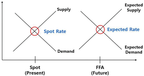The FFA rate is also influenced by the expectation of spot rate at the expiry date. Figure 1 shows this determination mechanism. The TC rate is the average of the current spot rate and the expectations of future spot rates. All these arguments can be formalized as the following equations:

Figure 1. Determination of spot and FFA rates.

Source: Authors

(10) $\mathrm{spot}\mathrm{rat}{\mathrm{e}}_t=\mathit{f}\left({\epsilon }_{\mathit{c},\mathit{t}},{\epsilon }_{\mathit{f},\mathit{t}},{\epsilon }_{\mathit{r},\mathit{t}}\right),$(10)

(11) $\mathrm{FF}{\mathrm{A}}_t=\mathrm{E}[\mathrm{spot}\mathrm{rat}{\mathrm{e}}_T|{\mathrm{I}}_t]$(11)

where ${\mathrm{I}}_t$ means the available information up to the time t

(12) $\mathrm{T}{\mathrm{C}}_t=1/1\mathit{T}\left(\mathrm{spot}\mathrm{rat}{\mathrm{e}}_t+{\sum }_{\tau =t+1}^T\mathrm{E}\left[\mathrm{spot}\mathrm{rat}{\mathrm{e}}_{\tau }|{\mathrm{I}}_t\right]\right)$(12)

where discount rate is assumed to be zero.

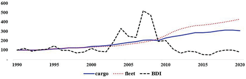
For the empirical examinations of the above theoretical arguments, this study uses the yearly dataset consisting of cargo transportation demand, ship supply, and freight rate in dry bulk shipping markets. It should be noted that, while the freight rate and ship supply variables are available at least on monthly frequency, the cargo demand variable (i.e. shipping amount of cargo) is available on yearly basis. So, this study assumes that the market mechanism observed on yearly dataset would function as well on more short frequencies, e.g. weekly case. In particular, the cargo volume data is world seaborne dry bulk trade in terms of metric ton, the ship supply is total bulk carrier fleet in terms of DWT (deadweight tons), and the freight rate is the BDI (Baltic Dry Index) published by the Baltic Exchange (Table 1).

Table 1. Summary of yearly dataset.

Cargo volume	Fleet	BDI (Freight rate)
World seaborne dry bulk trade (unit: ton)	Total bulk carrier fleet (unit: DWT)	Baltic Dry Index (unit: index)
Sample period: 1990 to 2020. Number of observations: 31

Source: Clarksons.

Figure 2 shows the movements of the three demand, supply, and price variables. The cargo volume and fleet size have increased continuously but the freight rate (BDI) have fluctuated responding to the balance between cargo demand and ship supply.

Figure 2. Movements of demand (cargo), supply (fleet), and price (BDI) in dry bulk shipping market.

Note: The values of the three variables in 1990 are set to be 100.

Source: Clarksons

Before the examination of the relationships among the three variables, this study conducts the unit root tests for the log-level and log-differenced data. The log-level data in Table 2 seem to be non-stationary, because the null hypothesis of unit root is not rejected at conventional significance levels, e.g. 1%, 5%, or 10%. However, the log-differenced data seem to be stationary at a significance level at least 13%. In short, the unit root tests allow us to use vector error correction model as an empirical estimation.

Table 2. Results of the unit root test for log-level and log-differenced data in yearly dataset.

log-level	Cargo volume	t-value	−0.46
		p-value	0.88
	Fleet	t-value	−0.31
		p-value	0.91
	BDI	t-value	−1.93
		p-value	0.31
log-differenced	Cargo volume	t-value	−4.57
		p-value	0.00***
	Fleet	t-value	−2.63
		p-value	0.09*
	BDI	t-value	−2.46
		p-value	0.13

Notes1) *, **, and *** indicate significance at the 10%, 5%, and 1% levels, respectively.

2) The t-statistic refers to the Augmented Dickey–Fuller test statistic.

3) For the log-level and log-differenced data, the test has a constant.

Source: Authors.

The cointegration test results in Table 3 mean that we cannot reject the null hypothesis that there is at most one cointegration relationship at the 1% significance level. Further, the estimated cointegrating vector shows that the increase of cargo demand leads to the BDI increase but the increase of ship supply leads to the BDI decrease. In addition, the estimation of adjustment coefficients implies that, when the BDI is above the long-run equilibrium level, the BDI and cargo volume decreases but the fleet increases. These properties mean that there are ‘long-run components of variables to obey equilibrium constraints’ (Engle and Granger 1987, 252).

Table 3. Results of cointegration tests and VECM estimation for yearly dataset.

Null hypothesis	Number of cointegration Relationship: none	Number of cointegration Relationship: at most 1
Cointegration rank test (trace)
Trace statistic	36.69	16.01
p-value	0.00***	0.04**
Cointegrating vector $\left[\begin{array}{cc}1& {\beta }_{\mathrm{\_}}\mathit{c}\end{array}\mathit{\beta }\_\mathit{f}\mathit{c}\right]$ such that $\left[1{\beta }_c{\beta }_f\mathit{c}\right]\left[\begin{array}{c}{b}_{\mathit{t}-1}\\ c_{\mathit{t}-1}\\ f_{\mathit{t}-1}\\ 1\end{array}\right]$	[1–3.73 0.34 2.03] (0.70) (0.55)
Adjustment coefficients
$b_t$	$c_t$	$f_t$
−0.73(0.27) ***	−0.07(0.02) ***	0.01(0.01)

Notes: 1) b_t means BDI, means cargo volume, and means fleet.

2) standard errors in parentheses.

3) *, **, and *** indicate significance at the 10%, 5%, and 1% levels, respectively.

Source: Authors.

The unit root tests confirm that the cargo, fleet, and rate variables follow random walk non-stationary stochastic process, which are modelled as the above Equations (7)(7) $\mathrm{B}{\mathrm{Y}}_{\mathrm{t}}=\mathit{\hspace{0.17em}}{\mathrm{\Gamma }}_1{\mathrm{Y}}_{\mathrm{t}-1}+\mathit{\hspace{0.17em}}{\mathrm{\Gamma }}_2{\mathrm{Y}}_{\mathrm{t}-2}+\mathit{\hspace{0.17em}}{\mathrm{E}}_{\mathrm{t}},$(7) and (8(8) $\mathrm{\Delta }{\mathrm{Y}}_{\mathrm{t}}=\mathrm{\Pi }{\mathrm{Y}}_{\mathrm{t}-1}+\mathit{\hspace{0.17em}}{\mathrm{\Pi }}_1{\mathrm{\Delta }\mathrm{Y}}_{\mathrm{t}}+\mathit{\hspace{0.17em}}{U}_{\mathrm{t}}.$(8) ). In addition, the estimated cointegrating vector confirms the price (freight rate) determination mechanism formalized in the Equation (9)(9) $\mathrm{rat}{\mathrm{e}}_t=\mathit{c}+{\beta }_c\times \mathrm{carg}{\mathrm{o}}_t+{\beta }_f\times \mathrm{flee}{\mathrm{t}}_t+z_t.$(9) .

The above theoretic and empirical examinations imply that the spot, FFA, and TC rates are the functions of ${\epsilon }_{\mathit{c},\mathit{t}}$, ${\epsilon }_{\mathit{f},\mathit{t}}$, ${\epsilon }_{\mathit{r},\mathit{t}}$ and $\mathrm{E}[{\epsilon }_{\mathit{c},\mathit{\tau }}|{\mathrm{I}}_t]$, $\mathrm{E}[{\epsilon }_{\mathit{f},\mathit{\tau }}|{\mathrm{I}}_t]$, $\mathrm{E}[{\epsilon }_{\mathit{r},\mathit{\tau }}|{\mathrm{I}}_t]$ for $\mathit{\tau }=\mathrm{t}+1,\mathit{\hspace{0.17em}}\dots ,\mathrm{J}$ where $\mathrm{J}$ is the end date of considered variables. The structural shocks of the first and second structural VAR models can be interpreted by using the elements of ${\epsilon }_{\mathit{c},\mathit{t}}$, ${\epsilon }_{\mathit{f},\mathit{t}}$, ${\epsilon }_{\mathit{r},\mathit{t}}$ and $\mathrm{E}[{\epsilon }_{\mathit{c},\mathit{\tau }}|{\mathrm{I}}_t]$, $\mathrm{E}[{\epsilon }_{\mathit{f},\mathit{\tau }}|{\mathrm{I}}_t]$, $\mathrm{E}[{\epsilon }_{\mathit{r},\mathit{\tau }}|{\mathrm{I}}_t]$. For the first structural VAR model, the permanent shock ${\epsilon }_{1\mathit{t}}$ influences all the shocks and their expectations such as ${\epsilon }_{\mathit{c},\mathit{t}}$, ${\epsilon }_{\mathit{f},\mathit{t}}$, ${\epsilon }_{\mathit{r},\mathit{t}}$ and $\mathrm{E}[{\epsilon }_{\mathit{c},\mathit{\tau }}|{\mathrm{I}}_t]$, $\mathrm{E}[{\epsilon }_{\mathit{f},\mathit{\tau }}|{\mathrm{I}}_t]$, $\mathrm{E}[{\epsilon }_{\mathit{r},\mathit{\tau }}|{\mathrm{I}}_t]$. As mentioned above, the long-term infrastructure investment decision can be this permanent shock ${\epsilon }_{1\mathit{t}}$, because it influences all the variables of FFA, spot, and TC rates. The second seasonal shock ${\epsilon }_{2\mathit{t}}$ influences only the current shocks such as ${\epsilon }_{\mathit{c},\mathit{t}}$, ${\epsilon }_{\mathit{f},\mathit{t}}$, ${\epsilon }_{\mathit{r},\mathit{t}}$. For example, the temporary rise of grain shipping volume in harvest season influences only the spot market so that this change can be this transitory shock ${\epsilon }_{2\mathit{t}}$. The third shock ${\epsilon }_{3\mathit{t}}$ influences the expectations of $\mathrm{E}[{\epsilon }_{\mathit{c},\mathit{\tau }}|{\mathrm{I}}_t]$, $\mathrm{E}[{\epsilon }_{\mathit{f},\mathit{\tau }}|{\mathrm{I}}_t]$, $\mathrm{E}[{\epsilon }_{\mathit{r},\mathit{\tau }}|{\mathrm{I}}_t]$. For the first structural VAR model, $\mathit{\tau }=\mathrm{t}+2,\mathit{\hspace{0.17em}}\dots ,\mathrm{J}$ and for the second VAR model, $\mathit{\tau }=\mathrm{t}+1,\mathit{\hspace{0.17em}}\dots ,\mathrm{J}$. These interpretations of ${\epsilon }_{1\mathit{t}}$, ${\epsilon }_{2\mathit{t}}$, and ${\epsilon }_{3\mathit{t}}$ allow us to use the two structural VAR models. For instance, the distant shock such as future large investment decision can be this structural shock ${\epsilon }_{3\mathit{t}}$.

However, the weekly variables should be checked to see if the use of VAR approach is appropriate. For this purpose, this study conducts the Granger causality test and the cointegration test. Table 4 shows the Granger–causality test results on log-level variables of spot, FFA, and TC rates (based on the dataset in Table 6). The results imply that there are dynamic interactions among the three variables. Further, although there is a jump problem in the FFA data, there are long-run equilibrium relationships among the variables (Table 5). In conclusion, the three variables VAR model of this present study is appropriate for the dry bulk shipping dataset. Further, all the theoretical and empirical examinations in the Subsections 3.1 and 3.2 show that the two structural VAR models of this study are exactly identified in the sense that the structural parameters can be recovered uniquely from the reduced-form parameters (Kilian and Lűtkepohl 2017, 173–174).

Table 4. Granger–causality test results of log-level FFA, spot, and TC rates.

-	Chi-sq. statistic	p-value
Spot → FFA	13.49	0.00***
TC → FFA	3.05	0.21
FFA → Spot	367.83	0.00***
TC → Spot	38.32	0.00***
FFA → TC	112.46	0.00***
Spot → TC	4.27	0.11

Note: *, **, and *** indicate significance at the 10%, 5%, and 1% levels, respectively.

Source: Authors.

Table 5. Results of cointegration tests for weekly dataset.

Null hypothesis	Number of cointegration Relationship: none	Number of cointegration Relationship: at most 1	Number of cointegration Relationship: at most 2
Cape
Trace statistic	89.44	31.64	4.03
p-value	0.00***	0.00***	0.04**
Panamax
Trace statistic	106.18	41.61	1.77
p-value	0.00***	0.00***	0.18
Supramax
Trace statistic	94.93	24.04	0.24
p-value	0.00***	0.00***	0.61

Note: *, **, and *** indicate significance at the 10%, 5%, and 1% levels, respectively.

Source: Authors.

3.3. Sizes of the variances of structural shocks

Equation (1)(1) $\mathrm{B}\mathrm{\Delta }{\mathrm{Y}}_{\mathrm{t}}=\mathit{\hspace{0.17em}}{\sum }_{i=1}^p{\mathrm{\Gamma }}_i\mathrm{\Delta }{\mathrm{Y}}_{\mathrm{t}-\mathrm{i}}+\mathit{\hspace{0.17em}}{\mathrm{E}}_{\mathrm{t}},$(1) assumes that the variances in structural shocks are all unity; that is, they are one. This means that normalization is done on the variances of the shocks. However, if one wants to calculate the size of the variances of structural shocks, then one can normalize on the dependent variables, which leads to the following equation:

(13) $B^{\ast }\mathrm{\Delta }{\mathrm{Y}}_{\mathrm{t}}=\mathit{\hspace{0.17em}}{\sum }_{i=1}^p{\mathrm{\Gamma }}_i^{\ast }\mathrm{\Delta }{\mathrm{Y}}_{\mathrm{t}-\mathrm{i}}\mathit{\hspace{0.17em}}+\mathit{\hspace{0.17em}}{E}_t^{\ast },$(13)

where $B^{\ast }\equiv \left[\begin{array}{ccc}1& {\mathrm{b}}_{12}^{\ast }& {\mathrm{b}}_{13}^{\ast }\\ {\mathrm{b}}_{21}^{\ast }& 1& {\mathrm{b}}_{23}^{\ast }\\ {\mathrm{b}}_{31}^{\ast }& {\mathrm{b}}_{32}^{\ast }& 1\end{array}\right],\mathrm{\Delta }{\mathrm{Y}}_{\mathrm{t}}\equiv \left[\begin{array}{c}\mathrm{\Delta }{\mathrm{y}}_{1\mathrm{t}}\\ \mathrm{\Delta }{\mathrm{y}}_{2\mathrm{t}}\\ \mathrm{\Delta }{\mathrm{y}}_{3\mathrm{t}}\end{array}\right],{\mathrm{\Gamma }}_i^{\ast }\equiv \left[\begin{array}{ccc}{\gamma }_{11,i}^{\ast }& {\gamma }_{12,i}^{\ast }& {\gamma }_{13,i}^{\ast }\\ {\gamma }_{21,i}^{\ast }& {\gamma }_{22,i}^{\ast }& {\gamma }_{23,i}^{\ast }\\ {\gamma }_{31,i}^{\ast }& {\gamma }_{32,i}^{\ast }& {\gamma }_{33,i}^{\ast }\end{array}\right],$ $\mathrm{and}$

$E_t^{\ast }\equiv \left[\begin{array}{c}{\epsilon }_{1t}^{\ast }\\ {\epsilon }_{2t}^{\ast }\\ {\epsilon }_{3t}^{\ast }\end{array}\right]\sim \mathrm{i}.\mathrm{i}.\mathrm{d}.\left[\begin{array}{cc}\left(\begin{array}{c}0\\ 0\\ 0\end{array}\right),& \left(\begin{array}{ccc}{\sigma }_1^2& 0& 0\\ 0& {\sigma }_2^2& 0\\ 0& 0& {\sigma }_3^2\end{array}\right)\end{array}\right]$

So, by using an estimated Equation (1)(1) $\mathrm{B}\mathrm{\Delta }{\mathrm{Y}}_{\mathrm{t}}=\mathit{\hspace{0.17em}}{\sum }_{i=1}^p{\mathrm{\Gamma }}_i\mathrm{\Delta }{\mathrm{Y}}_{\mathrm{t}-\mathrm{i}}+\mathit{\hspace{0.17em}}{\mathrm{E}}_{\mathrm{t}},$(1) , one can derive Equation (13)(13) $B^{\ast }\mathrm{\Delta }{\mathrm{Y}}_{\mathrm{t}}=\mathit{\hspace{0.17em}}{\sum }_{i=1}^p{\mathrm{\Gamma }}_i^{\ast }\mathrm{\Delta }{\mathrm{Y}}_{\mathrm{t}-\mathrm{i}}\mathit{\hspace{0.17em}}+\mathit{\hspace{0.17em}}{E}_t^{\ast },$(13) .

3.4. Beveridge-Nelson decomposition

Facing fluctuations in some variables, we often think these variabilities may stem from trends plus periodic cycles. In particular, the positive cycle term (above the assumed trend term) indicates there will be pressure for the variable to converge down to the trend, due to a boom cycle. In contrast, when the cycle term is negative below the trend term, the variable will converge up to the trend, due to a recession. Along with this logical thinking, B-N decomposition (into permanent trend and transitory cycle terms) can also provide significant information on the movement of the considered variables.

The optimal long-run forecast of B-N decomposition for the spot variables, i.e. $y_{2t}^p\mathit{\hspace{0.17em}}\equiv y_{2\mathit{t}}+\underset{\mathit{J}\to \mathrm{\infty }}{lim}{\sum }_{j=1}^J\mathit{E}[\mathrm{\Delta }{y}_{2\mathit{t}+\mathit{j}}|I_t]$, can be interpreted as an estimate of an unobserved permanent component of the considered integrated time series (the spot rates). For example, if this permanent term is greater than $y_{2\mathit{t}}$, then the future value is expected to increase. So, we can define the cyclical part of the time series as $y_{2t}^c\equiv \mathit{\hspace{0.17em}}{y}_{2\mathit{t}}-\mathit{\hspace{0.17em}}{y}_{2t}^p$. Based on this definition, this paper uses the following formula for calculating the cyclical component of the spot rates (see Morley 2002):

(14) $y_{2t}^c=-\underset{\mathit{J}\to \mathrm{\infty }}{lim}{\sum }_{j=1}^J\mathit{E}[\mathrm{\Delta }{y}_{2\mathit{t}+\mathit{j}}|I_t]$(14)

where $\underset{\mathit{J}\to \mathrm{\infty }}{lim}{\sum }_{j=1}^J\mathit{E}[\mathrm{\Delta }{y}_{2\mathit{t}+\mathit{j}}|I_t]\equiv 2\mathit{nd}\mathit{element}\mathit{of}\mathit{F}{\left({\mathit{I}}_{\left(3\times \mathit{p}\right)}-\mathit{F}\right)}^{-1}\left[\begin{array}{c}\mathrm{\Delta }{Y}_t\\ ⋮\\ \mathrm{\Delta }{Y}_{\mathit{t}-\mathit{p}+1}\end{array}\right]$

with $\mathrm{F}\equiv \left[\begin{array}{cccc}{\mathrm{\Phi }}_1& \cdots & {\mathrm{\Phi }}_{\mathit{p}-1}& {\mathrm{\Phi }}_p\\ I_3& 0_3& 0_3& 0_3\\ ⋮& \ddots & ⋮& ⋮\\ 0_3& 0_3& I_3& 0_3\end{array}\right]\mathit{\hspace{0.17em}}$.

Therefore, if $y_{2t}^c$ is positive, then the spot rate is expected to decrease. But if $y_{2t}^c$ is negative, the spot rate is expected to increase.

4. Results and implications

4.1. Data

4.1.1. Dataset

This study uses a dataset consisting of weekly spot, FFA, and TC rates in the Capesize, Panamax, and Supramax dry bulk shipping markets. A Capesize ship, at about 180,000 dead-weight tons (DWT), primarily transports iron ore; a Panamax ship (about 75,000 DWT) transports grain and coal, and Supramax ships (about 58,000 DWT) transport grain. The spot and FFA rates were obtained from Baltic Exchange, and the TC rates came from Clarksons Research. More specifically, the Capesize 5TC, Panamax 4TC, and Supramax 10TC rates were used as the spot rates, and their corresponding Baltic Forward Assessment (BFA) rates of 1 month prior to maturity were used as the FFA variables (for detailed information on each variable, refer to Baltic Exchange). The six-month TC rates were used as the TC variables. The spot rate represents the current price for transporting bulk cargoes.The FFA rate is a forward price for transporting cargoes at some future time without actual delivery. The starting point of the sample period differs across the considered markets. The Capesize period is from 4 July 2014; Panamax is from 7 January 2011; and Supramax is from 28 October 2016. Table 6 summarizes the dataset for this study.

Table 6. Summary of the weekly dataset.

–	Spot rate	FFA rate	TC rate	Sample period	Number of observations
Capesize	5TC Average of 5 freight rates for 180,000 DWT	1-month FFA for 5TC	6-month TC for 180,000 DWT	4^th Jul. 2014 ~ 24^th Sep. 2021	373
Panamax	4TC Average of 4 freight rates for 74,000 DWT	1-month FFA for 4TC	6-month TC for 75,000 DWT	7^th Jan. 2011 ~ 24^th Sep. 2021	552
Supramax	10TC Average of 10 freight rates for 58,000 DWT	1-month FFA for 10TC	6-month TC for 58,000 DWT	28^th Oct. 2016 ~ 24^th Sep. 2021	254

Source: Baltic Exchange and Clarksons Research.

The weekly average of the daily data was used for the spot rates. The final-day value of the week was used for the FFA rates because the latest assessment will reflect the most recent information on the corresponding FFA contracts. For the TC rates, the original data from Clarksons Research are weekly.

4.1.2. Basic properties and unit root tests of dataset

Figure 3 shows the movements of the spot, FFA, and TC rates in the Panamax markets and Table 7 shows the correlations among the rates for Capesize, Panamax, and Supramax markets. As seen in Subsection 4.2, these high correlations can be explained by the common influential permanent components (Also, see Ko 2018).

Figure 3. Movements of the weekly spot, FFA, and TC rates of panamax.

Source: Authors’ calculations from Baltic Exchange and Clarksons Research data.

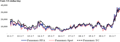
Table 7. Correlations among the spot, FFA, and TC rates of the three bulk markets.

–	Capesize			Panamax			Supramax
	FFA	Spot	TC	FFA	Spot	TC	FFA	Spot	TC
FFA	1	–	–	1	–	–	1	–	–
Spot	0.92	1	–	0.96	1	–	0.98	1	–
TC	0.96	0.92	1	0.96	0.95	1	0.99	0.99	1

Source: Authors’ calculations from Baltic Exchange and Clarksons Research data.

All values from the original data were transformed into natural logarithms. For log-level data, the null hypothesis is that a unit root exists in cases with a constant. If they cannot be rejected at the 1% significance level, it means the log-level variables are likely to be non-stationary. This non-stationarity prohibits the application of conventional statistical inference to the variables considered. But if we take the differences between logarithms of the variables, the null hypothesis for the existence of a unit root in cases without a constant or trend can be rejected at the 1% significance level. This means that log-differencing the non-stationary variables makes them stationary (Table 8). That is, the variables are all integrated at order 1, $\mathrm{I}\left(1\right)$. Even if there have been some controversies on the stationarities of shipping variables, this study used a log-differenced dataset to allow us to examine the dynamic relationships among the variables.

Table 8. Results of the unit root test for log-level and log-differenced data.

Capesize	log-level	FFA	t-value	−2.11
			p-value	0.23
		Spot	t-value	−3.94
			p-value	0.00***
		TC	t-value	−2.20
			p-value	0.20
	log-differenced	FFA	t-value	−18.44
			p-value	0.00***
		Spot	t-value	−12.28
			p-value	0.00***
		TC	t-value	−15.51
			p-value	0.00***
Panamax	log-level	FFA	t-value	−2.26
			p-value	0.18
		Spot	t-value	−2.24
			p-value	0.18
		TC	t-value	−1.63
			p-value	0.46
	log-differenced	FFA	t-value	−24.31
			p-value	0.00***
		Spot	t-value	−12.66
			p-value	0.00***
		TC	t-value	−17.22
			p-value	0.00***
Supramax	log-level	FFA	t-value	0.05
			p-value	0.96
		Spot	t-value	−0.95
			p-value	0.76
		TC	t-value	0.20
			p-value	0.97
	log-differenced	FFA	t-value	−14.80
			p-value	0.00***
		Spot	t-value	−7.56
			p-value	0.00***
		TC	t-value	−8.09
			p-value	0.00***

Notes: 1) *, **, and *** indicate significance at the 10%, 5%, and 1% levels, respectively.

2) The t-statistic refers to the Augmented Dickey–Fuller test statistic.

3) For the log-level data, the test has a constant. But for the log-differenced data, the test does not have a constant or trend.

Source: Authors.

However, nearing the maturity date, the FFA time-series data show a jumping problem. For example, at the end of January, the FFA rate 1 month before maturity changes from FFA February to FFA March. That is, the underlying assets of FFA contracts will change so the time-series FFA rate 1 month before maturity represents the expected values of different future spot rates. So, for log-differencing the FFA data, there should be a cautious method to overcome this structural break problem. There are several alternative methods in the literature (e.g. see Kavussanos and Nomikos 2003, 207–209). One of most popular methods is using a perpetual FFA contract, which is an artificially weighted average of near and distant FFA contracts (Kavussanos and Visvikis 2004). Despite this received good method, this study uses an innovative and simple method to address this structural problem and transform the FFA data into stationary data. The reason for using the alternative method is that for perpetual FFA prices, it is possible to average out the relevant information that occurred at the time considered. For example, if significant information has a big influence on the near FFA but not on the distant FFA or vice versa, then the perpetual FFA price would incorporate less information than the actual FFA price.

When using the FFA data for VAR analysis, we typically log-difference the variables, giving them stationarity, except that a VECM uses the log-level variables in order to utilize their long-run relationships. However, this paper uses only the VAR model. As the results of the unit root test imply, we also need a set of only log-differenced data for VAR analysis. So, for the FFA data, we can calculate the consistent log-differenced values without a perpetual FFA contract. That is, for example, at the end of January, instead of using FFA February of the last period and FFA March of the current period, we can use only the two FFA March rates from the last and current periods in order to calculate the log-differenced value. This method ensures consistency in the log-differenced FFA time-series data, because it uses the same underlying asset for the corresponding BFA. To the best of our knowledge, only Kavussanos, Visvikis, and Dimitrakopoulo (2010, 86) adopted this new and simple method.

Figure 4 shows the movements of the log-differenced data on weekly spot, FFA, and TC rates for Panamax markets, and Table 9 shows the correlations among the rates for Capesize, Panamax, and Supramax markets. In contrast to the original data, their correlations are much lowered. In particular, the correlations between the spot and FFA rates are the lowest. These low correlations indicate that log-differencing may have removed some common stochastic components among them.

Figure 4. Movements of the log-differenced data of weekly panamax spot, FFA, and TC rates.

Source: Authors’ calculations from Baltic Exchange and Clarksons Research data.

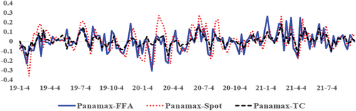
Table 9. Correlations of log-differenced data for the spot, FFA, and TC rates in the three bulk markets.

–	Capesize			Panamax			Supramax
	FFA	Spot	TC	FFA	Spot	TC	FFA	Spot	TC
FFA	1	–	–	1	–	–	1	–	–
Spot	0.46	1	–	0.28	1	–	0.25	1	–
TC	0.72	0.57	1	0.58	0.64	1	0.50	0.56	1

Source: Authors’ calculations from Baltic Exchange and Clarksons Research data.

4.1.3. Optimal lag length and diagnostic tests

Table 10 shows the optimal lag length selected by AIC (Akaike information criterion), SC (Schwarz information criterion), and HQ (Hannan-Quinn information criterion). For the Capesize, the SC and HQ recommend the lag length as one and for the Panamax, lag length is recommended as two. For the Supramax case, all the three criteria recommend the lag length as two. So, this study sets the lag length as one for Capesize and two for the Panamax and Supramax.

Table 10. Optimal lag length selected by AIC, SC, and HQ criteria.

Capesize			Panamax			Supramax
AIC	SC	HQ	AIC	SC	HQ	AIC	SC	HQ
9	1	1	6	2	2	2	2	2

AIC means Akaike information criterion, SC means Schwarz information criterion, HQ means Hannan-Quinn information criterion.

Source: Authors.

Table 11 shows the LM (Lagrange Multiplier) test results for the null hypothesis that there is no serial correlation in the error terms. For the Capesize and Supramax cases, there is no autocorrelation. However, for the Panamax case, the null hypothesis of no autocorrelation is rejected at 1% significance level, which does not seem to be consistent with the optimal lag length selection. The selection criteria are based on searching the optimal lag that balances the objectives of model fit and parsimony, which typically leads to no autocorrelation in errors. The Panamax case in which the optimal lag cannot guarantee no autocorrelation in errors might be a limitation of the above criteria such as AIC, SC, and HQ. To overcome this limitation remains as a future research topic.

Table 11. LM tests for no autocorrelation in error terms.

Capesize		Panamax		Supramax
Lag length = 1		Lag length = 2		Lag length = 2
LM-stat	p-value	LM-stat	p-value	LM-stat	p-value
12.98	0.16	31.23	0.00	12.31	0.19

Source: Authors.

Table 12 presents the results of the White heteroskedasticity test, which tests the null hypothesis of homoskedasticity. The test indicates rejection of the homoskedasticity hypothesis, suggesting the presence of heteroskedasticity. However, it is important to note that heteroskedasticity does not affect the consistency of estimated coefficients (Greene 2003, 194–195), so the results of point estimates and their interpretations presented in this paper remain valid.

Table 12. White heteroskedasticity (null hypothesis: no heteroskedasticity) tests in covariance matrix.

Capesize		Panamax		Supramax
Chi-square	p-value	Chi-square	p-value	Chi-square	p-value
115.96	0.00	132.08	0.00	131.65	0.00

Source: Authors.

4.2. Two structural VAR models

Figure 5 shows the accumulated impulse response analyses from the first structural VAR model, i.e. the recursive VAR model. First, the Physical-Paper Hypothesis, where FFA rates respond more rapidly to new information than spot and TC rates, is well supported by the empirical results. The FFA rates respond particularly promptly to the first permanent shock (blue lines of the first column). But the responses of the spot and TC rates increase gradually (blue lines of the second and third columns, respectively). We interpret these phenomena as supporting the Physical-Paper Hypothesis. In addition, it should be noted that there is some difference in the propagation speed of permanent shock. According to the figures in the second columns, Capesize’s spot rate more quickly reaches to the upper level than those of Panamax and Supramax, and Panamax responds more rapidly than Supramax. This means that larger ship size more quickly responds to the permanent shock than smaller ship sizes as the former may have more reactive capacity to potential risks. This tendency may stem from the fact that larger ships tend to be involved in narrower transportation markets in terms of cargo types, shipping routes, etc. That is, the narrowness of larger ships can cause them to respond to new shocks more rapidly because of the simplicity of involved market conditions.

Figure 5. Accumulated impulse response analyses of structural VAR model 1.

The blue lines are responses to permanent shock, the dotted red lines to seasonal shock, and the dashed black lines to post—two-period permanent shock. The horizontal axis means the considered periods and the vertical axis measures the responses of logarithmic values of the considered variables.

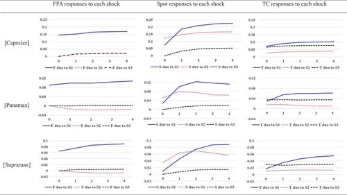
Second, there are two notable dynamic patterns to the Shock-Diversity Hypothesis. One pattern is that, in all the nine cases, the permanent shock has the most influence on the three variables. So, according to the first structural VAR model, one can conclude that the most influential shock on dry bulk shipping markets is the permanent one, which may be regarded as the main cause for the high correlations among the variables seen in Figure 3. The second pattern is that, in each market (variable), the three structural shocks have their characteristic roles. That is, the permanent shock is dominant in FFA response. In contrast, in spot response, the influence of the seasonal shock is more significant than in FFA response and, in TC response, the post-two-period permanent shock becomes more influential.

The results of this study corroborate these two properties i) that FFA rates respond more rapidly than spot and TC rates and ii) that the structurally identified shocks have their characteristic propagation mechanisms as supporting the Physical-Paper hypothesis and Shock-Diversity hypothesis at the same time.

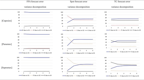
Figure 6 depicts the forecast error variance decompositions of the first structural VAR model. As implied from the impulse response analysis, most of the FFA forecast errors come from permanent shocks. In the spot and TC rates, the contributions of seasonal and post-two-period permanent shocks becomes larger than in FFA cases, respectively. In other words, the seasonal shock becomes more important in predicting spot rate and the post-two-period shock becomes more important in predicting TC rate. This larger contribution of transitory seasonal shock in forecasting spot rates helps us to forecast the future spot rates by using the past observed data.

Figure 6. Forecast error variance decomposition of structural VAR model 1.

The blue lines are the fraction of the forecast error due to permanent shock, the dotted red lines are the error due to seasonal shock, and the dashed black lines are the error due to post—two-period permanent shock. The horizontal axis means the considered periods and the vertical axis measures the percentage portions of the considered shocks in the forecast errors.

Figure 7 shows the accumulated impulse response analyses of the second structural VAR model with short-run and long-run restrictions. Overall, the dynamic propagation mechanisms of the structural shocks are different from those of the first structural model. For example, for the FFA in the two markets, the most influential shock is not the permanent shock, as in the first model; it is the post-one-period permanent shock.

Figure 7. Accumulated impulse response analyses from structural VAR model 2.

The blue lines are for responses to permanent shock, the dotted red lines, to seasonal shock, and the dashed black lines, to post—one-period permanent shock. The horizontal axis means the considered periods and the vertical axis measures the responses of logarithmic values of the considered variables

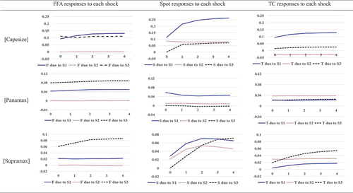
Regarding the Physical-Paper Hypothesis, like the first structural VAR model, the results of the second structural VAR model show that FFA rates respond promptly to the two permanent shocks, but the responses in spot rates increase gradually. In addition, regarding the Shock-Diversity Hypothesis, two dynamic patterns can be observed. One is that the permanent and post-one-period permanent shocks have more influence than the seasonal shock. The second is that while the seasonal shock causes significant spot responses in Capesize and Supramax markets, the permanent shock causes more significant spot responses in Panamax market, which is different from the first structural VAR model. In addition, it is notable that, as the long-run neutrality restriction imposes, the responses of FFA rates to the seasonal shock are about zero.

Tables 13 and Table 14 show the standard deviations for each structural shock under the two structural VAR models (see Equation 13(13) $B^{\ast }\mathrm{\Delta }{\mathrm{Y}}_{\mathrm{t}}=\mathit{\hspace{0.17em}}{\sum }_{i=1}^p{\mathrm{\Gamma }}_i^{\ast }\mathrm{\Delta }{\mathrm{Y}}_{\mathrm{t}-\mathrm{i}}\mathit{\hspace{0.17em}}+\mathit{\hspace{0.17em}}{E}_t^{\ast },$(13) ). As expected from the analyses in Figures 5–7, the most volatile shock is the permanent one, which also implies that the permanent shock is the most influential and the main cause for the high correlations among the considered variables. In addition, the Capesize market is most volatile. However, the differences in the identification restrictions on seasonal shocks yield the different results for the size of each of structural shocks.

Table 13. Standard deviations for each structural shock under structural VAR model 1.

–	Capesize		Panamax		Supramax
	standard deviation	% to A	standard deviation	% to A	standard deviation	% to A
Permanent shock	0.1440 (A)	100%	0.0911 (A)	100%	0.0657 (A)	100%
Seasonal shock	0.1226	85%	0.0571	63%	0.0394	60%
Post—two-period shock	0.0660	46%	0.0352	39%	0.0296	45%

Source: Authors.

Table 14. Standard deviations for each structural shock under structural VAR model 2.

–	Capesize		Panamax		Supramax
	standard deviation	% to A	standard deviation	% to A	standard deviation	% to A
Permanent shock	0.9865 (A)	100%	0.7951 (A)	100%	0.0397 (A)	100%
Seasonal shock	0.1257	13%	0.0868	11%	0.0357	90%
Post—one-period shock	0.1456	15%	0.3926	49%	0.0104	26%

The sizes of standard deviation of permanent shocks in Capesize and Panamax cases are noticeably large. However, the total influence of the structural shock depends on both of the size of standard deviation and the contemporaneous correlations measured by the elements of $B^{-1}$. So, this apparent anomaly of large variance can be resolved in the aspects of total influence of structural shocks.

Source: Authors.

4.3. Forecasting accuracy of the reduced-form VAR model

According to Stopford (2009, 742), the forecasting task to predict shipping markets is not to predict precisely, but to reduce uncertainty and help decision-makers understand the future. Accepting this wisdom, this study forecasts the weekly spot rates by using the reduced-form VAR model.

4.3.1. Forecasting accuracy using forecasting error information of the reduced-form VAR model

In this subsection, the forecasting accuracy is evaluated by RMSE (root mean square error), MAE (mean absolute error), MASE (mean absolute scaled error), and Theil’s inequality coefficient. These measures are defined as follows:

$\mathrm{RMSE}=\mathit{\hspace{0.17em}}\sqrt{\frac{1}{T}\mathit{\hspace{0.17em}}{\sum }_{t=1}^T{e}_t^2},\mathrm{MAE}=\mathit{\hspace{0.17em}}\frac{1}{T}{\sum }_{t=1}^T\left|e_t\right|,\mathrm{MASE}=\mathit{\hspace{0.17em}}\frac{1}{J}\left({\sum }_{j=1}^J\frac{\left|e_j\right|}{\frac{1}{\mathit{T}-1}{\sum }_{t=2}^T\left|Y_t-Y_{\mathit{t}-1}\right|}\right)$, and

$\mathrm{Thei}{\mathrm{l}}^{\prime }\mathrm{s}\mathrm{inequality}\mathrm{coefficient}=\mathit{\hspace{0.17em}}\frac{\sqrt{\frac{1}{T}{\sum }_{t=1}^T{\left(e_t\right)}^2}}{\sqrt{\frac{1}{T}{\sum }_{t=1}^T{\left(y_t^F\right)}^2}+\sqrt{\frac{1}{T}{\sum }_{t=1}^T{\left(y_t\right)}^2}}.$

Table 15 shows the spot rate forecasting accuracies of the tri-variate VAR and bi-variate VAR models in the in-sample context, based on the above four criteria. In all three markets, the tri-variate FFA-Spot-TC VAR model outperforms the bi-variate FFA-Spot and TC-Spot VAR models (for a similar result, see Zhang, Zeng, and Zhao 2014, 3646–3647). In particular, as to the comparisons between the tri-variate FFA-Spot-TC model and the bi-variate FFA-Spot model, the improvement rate is highest in the Capesize market.

Table 15. In-sample comparisons of forecasting accuracy between VAR models.

	RMSE	MAE	MASE	Theil’s coefficient
Capesize
FFA-Spot-TC VAR (A)	0.1424	0.1025	0.6810	0.4568
FFA-Spot VAR (B)	0.1461	0.1066	0.7080	0.4754
Improvement: (A-B)/B	−2.5%	−3.8%	−3.8%	−3.9%
TC-Spot VAR(C)	0.1505	0.1097	0.7289	0.4990
Improvement: (A-C)/C	−5.4%	−6.6%	−6.6%	−8.5%
Panamax
FFA-Spot-TC VAR (A)	0.0581	0.0443	0.5536	0.3113
FFA-Spot VAR (B)	0.0589	0.0449	0.5615	0.3170
Improvement: (A-B)/B	−1.5%	−1.4%	−1.4%	−1.8%
TC-Spot VAR(C)	0.0747	0.0576	0.7194	0.4341
Improvement: (A-C)/C	−22.3%	−23.1%	−23.1%	−28.3%
Supramax
FFA-Spot-TC VAR (A)	0.0359	0.0261	0.6308	0.2890
FFA-Spot VAR (B)	0.0367	0.0268	0.6477	0.2970
Improvement: (A-B)/B	−2.3%	−2.6%	−2.6%	−2.7%
TC-Spot VAR(C)	0.0421	0.0315	0.7597	0.3511
Improvement: (A-C)/C	−14.7%	−17.0%	−17.0%	−17.7%

Note: RMSE means root mean square error, MAE means mean absolute error, MASE means mean absolute scaled error, and Theil’s coefficient means Theil’s inequality coefficient.

Source: Authors.

Table 16 shows the spot rate forecasting accuracies of the tri-variate VAR and bi-variate VAR models in the out-of-sample context. For the Capesize and Panamax cases, the tri-variate VAR model outperforms the bi-variate VAR models, based on all the four criteria. However, for the Supramax case, the comparison results between the tri-variate FFA-spot-TC model and bi-variate FFA-Spot model are mixed evenly. On the other hand, the FFA-Spot model outperforms the TC-Spot model, which implies that FFA variable is more useful in forecasting future spot rates than TC variable.

Table 16. Out-of-sample comparisons of forecasting accuracy between VAR models.

	RMSE	MAE	MASE	Theil’s coefficient
Capesize
FFA-Spot-TC VAR (A)	0.1450	0.1014	0.6737	0.4483
FFA-Spot VAR (B)	0.1495	0.1058	0.7026	0.4681
Improvement: (A-B)/B	−3.0%	−4.1%	−4.1%	−4.2%
TC-Spot VAR(C)	0.1511	0.1102	0.7319	0.4918
Improvement: (A-C)/C	−4.0%	−7.9%	−7.9%	−8.9%
Panamax
FFA-Spot-TC VAR (A)	0.0630	0.0468	0.5847	0.3069
FFA-Spot VAR (B)	0.0640	0.0476	0.5949	0.3113
Improvement: (A-B)/B	−1.5%	−1.7%	−1.7%	−1.4%
TC-Spot VAR(C)	0.0756	0.0570	0.7130	0.4430
Improvement: (A-C)/C	−16.7%	−18.0%	−18.0%	−30.7%
Supramax
FFA-Spot-TC VAR (A)	0.0441	0.0330	0.7965	0.2447
FFA-Spot VAR (B)	0.0442	0.0327	0.7896	0.2516
Improvement: (A-B)/B	−0.2%	0.9%	0.9%	−2.7%
TC-Spot VAR(C)	0.0511	0.0384	0.9266	0.2981
Improvement: (A-C)/C	−13.7%	−14.0%	−14.0%	−17.9%

Notes: 1) RMSE means root mean square error, MAE means mean absolute error, MASE means mean absolute scaled error, and Theil’s coefficient means Theil’s inequality coefficient.

2) The period for out-of-sample forecasting in Capesize and Panamax markets is from Jan. 2018 to Sep. 2021; for the Supramax market, it is Jan. 2019 to Sep. 2021.

Source: Authors.

4.3.2. Direction forecasting of the reduced-form VAR model and B-N decomposition

In this subsection, the forecasting performance is evaluated by the success rate in forecasting the direction of the spot rate change. Table 17 compares forecasting directions from VAR and VAR B-N decomposition methods. First, the tri-variate FFA-Spot-TC VAR model outperforms the bi-variate FFA-Spot and TC-Spot VAR models in the Capesize and Panamax markets. However, in the Supramax market, the bi-variate FFA-Spot model forecast is slightly better than the tri-variate model, which deserves future research effort. VAR and VAR B-N decomposition have similar forecasting performance, because the forecast directions under both models are almost the same

Table 17. Comparisons of forecast directions with the VAR and VAR B-N methods.

–		Capesize	Panamax	Supramax
FFA-Spot VAR (A)	Right	146	164	117
	%	75.3%	84.5%	82.4%
TC-Spot VAR (B)	Right	143	153	103
	%	73.7%	78.9%	72.5%
FFA-Spot-TC VAR (C)	Right	151	166	116
	%	77.8%	85.6%	81.7%
B-N decomposition of FFA-Spot-TC VAR (D)	Right	150	159	107
	%	77.3%	82.0%	75.4%
C & D	Same	193	181	123
	%	99.5%	93.3%	86.6%
Total		194	194	142

Notes: 1) The period for out-of-sample forecasting in Capesize and Panamax markets is from Jan. 2018 to Sep. 2021; for the Supramax market, it is Jan. 2019 to Sep. 2021.

2) B-N method = Beveridge-Nelson decomposition.

3) C&D means the cases in which the FFA-Spot-TC VAR model and B-N method of tri-variate yield the same direction.

Source: Authors.

4.3.3. Signals conditional on the forecasts generated by the VAR model

Based on the results in Table 18, one can predict the direction of the spot rate changes, conditional on separate information generated by the VAR model with lag one. For the exposition, consider the following forecasting equation based on Equation (2)(2) $\mathrm{\Delta }{\mathrm{Y}}_{\mathrm{t}}=\mathit{\hspace{0.17em}}{\sum }_{i=1}^p{\mathrm{\Phi }}_i\mathrm{\Delta }{\mathrm{Y}}_{\mathrm{t}-\mathrm{i}}+\mathit{\hspace{0.17em}}{\mathrm{U}}_{\mathrm{t}}$(2) :

Table 18. Comparisons of forecasting directions based on signals conditional on the forecasts generated by the VAR model.

–		Capesize	Panamax	Supramax
Three variables have the same direction as the forecast	Total (A)	114	99	71
	Right (B)	95	91	62
	B/A	83%	92%	87%
Two variables have the same direction as the forecast	Total (A)	65	63	48
	Right (B)	46	52	37
	B/A	71%	83%	77%
One variable has the same direction as the forecast	Total (A)	15	32	23
	Right (B)	10	22	16
	B/A	67%	69%	70%

Note: The forecasting period in Capesize and Panamax markets is from Jan. 2018 to Sep. 2021; for the Supramax market, it is Jan. 2019 to Sep. 2021.

(15) $\mathrm{\Delta }{y}_{2t}^F={\varphi }_{21}\mathrm{\Delta }{y}_{1\mathit{t}-1}+{\varphi }_{22}\mathrm{\Delta }{y}_{2\mathit{t}-1}+{\varphi }_{23}\mathrm{\Delta }{y}_{3\mathit{t}-1}$(15)

Using Equation (15)(15) $\mathrm{\Delta }{y}_{2t}^F={\varphi }_{21}\mathrm{\Delta }{y}_{1\mathit{t}-1}+{\varphi }_{22}\mathrm{\Delta }{y}_{2\mathit{t}-1}+{\varphi }_{23}\mathrm{\Delta }{y}_{3\mathit{t}-1}$(15) , one can classify all cases as one out of three types. The first type is when all terms have the same direction (i.e. sign). The second is when the two terms on the right-hand side have the same sign as the forecast result, $\mathrm{\Delta }{y}_{2t}^F$. The third is when only one term on the right-hand side has the same sign as $\mathrm{\Delta }{y}_{2t}^F$.

Table 18 shows the comparisons of forecast directions based on the signals generated by the VAR model. The most accurate case is when the three variables have the same direction as the forecast value in the Panamax market (a success rate of 92%). The second highest group, with a success rate of 80% to 90%, consists of the cases where the three variables have the same direction as the forecast value in the Capesize and Supramax markets, and where the two variables have the same direction as the forecast value in the Panamax market. The third highest group, with a success rate of 70% to 80%, is where the two variables have the same direction as the forecast value in the Capesize and Supramax, and where one variable has the same direction as the forecast value in the Supramax market.

4.4. Implications

The major findings and their implications are summarized as follows.

First, as with macroeconometrics, this paper shows that the VAR methodology can work well for data description and structural inference in the dry bulk shipping markets based on the impulse response analysis and forecast error variance decomposition of structural VAR models. In particular, the empirical results of this study show that permanent shocks, such as news about launching a large investment for infrastructure or residential construction, are the most influential, contributing to high correlations among the variables considered. In addition, for the first structural VAR model, seasonal shocks become more important in spot rate response than in FFA response. These characterizations of dynamic patterns in dry bulk shipping markets can be interpreted as corroborating the Shock-Diversity Hypothesis.

Second, this study shows that the seemingly separate Physical-Paper Hypothesis and Shock-Diversity Hypothesis can be combined at one time in the structural VAR models. For example, the impulse response analyses show that the FFA rates respond more rapidly to permanent shocks than the spot rates, which supports the Physical-Paper Hypothesis. That is, due to market friction, such as an asymmetry in transaction costs or market microstructure effects, there are different dynamic response patterns in the spot and FFA rates to new information (e.g. Kavussanos and Visvikis 2004, 2016). Also, while permanent shocks are the main shocks in all three bulk shipping markets, the three structural shocks have their characteristic roles in each corresponding market, which verifies the Shock-Diversity Hypothesis.

Third, the combination of the Physical-Paper Hypothesis and the Shock-Diversity Hypothesis in this study suggests an important interpretation for the predictability of spot and futures rates. For example, Batchelor, Alizadeh, and Visvikis (2007) showed the spot rates can be forecast, but FFA rates are difficult to predict. However, these different predictabilities have not been explained in the literature yet. According to the results in Figure 6, most of the uncertainties in predicting FFA rates are due to permanent shocks. A permanent shock is defined as a factor that influences all three variables (i.e. FFA, spot, and TC rates) contemporaneously. These empirical results mean that the unpredictability of futures (FFA) rates comes from permanent shocks. In addition, the spot rates respond gradually to a permanent shock. Moreover, spot rates are relatively more influenced by seasonal shocks than FFA and TC rates. The gradualness of the spot rate’s response to permanent shocks, and the relatively more influential role of seasonal shocks, can lead to predictability of spot rates. Furthermore, TC rates can also be forecast because they exhibit gradualness in their responses to permanent shocks in the Panamax and Supramax markets.

Fourth, this study shows that the tri-variate FFA-Spot-TC VAR model can help market participants in weekly forecasting. Based on the four criteria, the tri-variate VAR model outperformed the bi-variate model in Capesize and Panamax cases, which is the same as the one from Zhang, Zeng, and Zhao (2014). Plus, the Capesize and Panamax tri-variate VAR model had a higher success probability when predicting the direction of the future spot rates. This paper also provides direction signals conditional on the forecasts generated by the VAR model. For instance, shipping operators can use this forecasting tool as an indicator for the best choice in charter contracting time.

5. Conclusion

This paper applies two illustrative structural vector autoregression models to the dry bulk shipping markets. The results consistently support both the Physical-Paper Hypothesis and the Shock-Diversity Hypothesis within the framework of one structural VAR model. The former hypothesis is particularly supported by the fact that the FFA rates respond more quickly than spot rates to permanent shocks. The latter hypothesis is confirmed by the pattern where a variety of structural shocks have corresponding diverse dynamic propagation mechanisms. This simultaneous corroboration of two hypotheses can resolve the predictability and unpredictability issues regarding FFA, spot, and TC rates. In addition, the reduced-form VAR model is shown to be useful as a forecasting tool for the practical chartering strategies of dry bulk market participants.

Four important topics not dealt with in this study are avenues for future research. First, because it is very fruitful to use a co-integrated VAR model in the case where certain long-run relationships exist among the considered variables, a VECM for the bulk shipping market should be developed. To develop a VECM in a bulk shipping market, FFA time-series data should be compiled. (Kavussanos and Nomikos 2003, 207–209) showed no significant differences in the methods of the perpetual FFA and the simple FFA 1 month before maturity. However, the structural break problem was not resolved suitably. So, to develop an acceptable method of constructing FFA time-series data deserves more research. Furthermore, based on this FFA data, the application of a time-varying co-integration model would be helpful for improving forecast performance. By the way, if we are interested only in the adjustment mechanisms to the temporary error terms, then we can construct the relevant manipulated long-run relationship between the spot and newly-constructed FFA rates, which is particularly expected to enhance the forecasting accuracy of considered models. Second, the structural VAR models based on prior beliefs about the signs of the effects of the shocks can be an alternative approach. This VAR model with sign restrictions, developed by, for example, Faust (1998), triggered a number of subsequent research efforts. In particular, Baumeister and Hamilton (2015) strongly argued that ‘explicitly defending the prior information used in the analysis and reporting the way in which the observed data caused these prior beliefs to be revised is superior to pretending that prior information was not used and has no effect on the reported conclusions’ (1993). By adhering to their recommendations, we can enhance our understanding of the market dynamics in a more econometrically rigorous manner. For instance, in the Bayesian approach, researchers or analysts can be provided with prior beliefs before observing the data. Unlike the standard frequentist VAR analysis, which is unable to incorporate this prior information (due to issues like the fallacy of base-rate neglect), the Bayesian method can effectively utilize such information. Consequently, market participants with abundant information, such as major shippers, ship operators, and investors, stand to gain an advantage by leveraging this prior knowledge. Third, analysis of the time pattern in structural shocks would be fruitful. For example, Kilian and Lűtkepohl (2017, 116–123) showed that the structural VAR model with the evolution of structural shocks and their contribution to the considered variables (so-called historical decomposition) can be a helpful tool for understanding the crude oil market. Similar to this, the historical evolution of structural shocks in bulk shipping markets may show some interesting patterns and interpretations. For example, based on this historical decomposition, we can distinguish the contributions of each structural shock at every point in the considered time span. Furthermore, just as Kavussanos and Visvikis (2004) used it, the VECM-GARCH approach can provide pattern information on dynamic volatilities. This conditional time-varying volatility measure might enhance the risk management of market participants. Fourth, Abouarghoub, Nomikos, and Petropoulos (2018) showed that their proposed hierarchical model based on a univariate ARIMA model improved forecasting performance. This forecasting improvement is thought to stem from their incorporation of the inherent correlation structure of the hierarchy in the considered shipping markets, i.e. specific shipping routes and services. So, multivariate extension of a hierarchical model, such as VAR or VECM, will enhance forecasting performance, because these multivariate models can assimilate other key market information. Further, it will be beneficial to use the concept of temporal hierarchy as Abouarghoub, Nomikos, and Petropoulos (2018) suggested.

To summarize, all four topics can effectively be addressed using a single structural multivariate time-series model. The construction of FFA dataset will help to extract the information of the derivatives markets. The utilization of a Bayesian VAR model with sign restrictions can significantly enhance the precision of updating our understanding of the markets under consideration. The time-varying measures for the (structural) shocks, e.g. historical decomposition or conditional volatilities, will provide us with the more accurate information on the fundamental market uncertainties. The final task to use categorical and temporal hierarchies will improve our (forecasting) methodologies by incorporating the complex relationships among the considered variables. In our future work, we will leverage a consistent FFA-level dataset compiled using an acceptable method. We plan to construct Bayesian structural VECMs with sign restrictions and the corresponding hierarchical model, incorporating categorical and temporal hierarchies. This approach aims to yield valuable and informative results.

Acknowledgments

We would like to express our warm thanks and appreciation to the Editor, Associate Editor and two anonymous reviewers for their helpful comments and suggestions on previous drafts of the paper, which substantially improved its quality. Ko greatly appreciates Prof. Chang-Jin Kim for his invaluable encouragement and instructions of econometrics in his graduate education. All inconsistencies and remaining errors are all on us.

Disclosure statement

No potential conflict of interest was reported by the author(s).

Additional information

Funding

This work was supported by funds from “Project of Center Operation for Forecasting Business Cycles in Shipping Industry” of Korea Maritime Institute.

References

- Abouarghoub, W., N. K. Nomikos, and F. Petropoulos. 2018. “On Reconciling Macro and Micro Engery Transport Forecasts for Strategic Decision Making in the Tanker Industry.” Transportation Research Part E: Logistics & Transportation Review 113:225–238. https://doi.org/10.1016/j.tre.2017.10.012.
- Adland, R., and A. H. Alizadeh. 2018. “Explaining Price Differences Between Physical and Derivative Freight Contracts.” Transportation Research Part E: Logistics & Transportation Review 118:20–33. https://doi.org/10.1016/j.tre.2018.07.002.
- Adland, R., L. E. Anestad, and B. Abrahamsen. 2023. “Statistical Arbitrage in the Freight Options Market.” Maritime Policy & Management 50 (2): 141–156. https://doi.org/10.1080/03088839.2021.1975055.
- Adland, R., and K. Cullinane. 2005. “A Time-Varying Risk Premium in the Term Structure of Bulk Shipping Freight Rates.” Journal of Transport Economics and Policy 39 (2): 191–208.
- Alizadeh, A. H., R. O. Adland, and S. Koekebakker. 2007. “Predictive Power and Unbiasedness of Implied Forward Charter Rates.” Journal of Forecast 26 (6): 385–403. https://doi.org/10.1002/for.1029.
- Amisano, G., and C. Giannini. 1997. Topics in Structural VAR Econometrics. Heidelberg: Springer-Verlag.
- Batchelor, R., A. Alizadeh, and I. Visvikis. 2007. “Forecasting Spot and Forward Prices in the International Freight Market.” International Journal of Forecast 23 (1): 101–114. https://doi.org/10.1016/j.ijforecast.2006.07.004.
- Baumeister, C., and J. D. Hamilton. 2015. “Sign Restrictions, Structural Vector Autoregressions, and Useful Prior Information.” Econometrica 83 (5): 1963–1999. https://doi.org/10.3982/ECTA12356.
- Bernanke, B. 1986. “Alternative Explanations of the Money-Income Correlation.” Carnegie-Rochester Conference Series on Public Policy, 25: 49–100. https://doi.org/10.1016/0167-2231(86)90037-0.
- Beveridge, S., and C. R. Nelson. 1981. “A New Approach to Decomposition of Economic Time Series into Permanent and Transitory Components with Particular Attention to Measurement of the ‘Business Cycle’.” Journal of Monetary Economics 7 (2): 151–174. https://doi.org/10.1016/0304-3932(81)90040-4.
- Blanchard, O. J., and D. Quah. 1989. “The Dynamic Effects of Aggregate Demand and Supply Disturbances.” American Economic Review 79 (4): 655–673.
- Blanchard, O. J., and M. W. Watson. 1986. “Are Business Cycles All Alike?” In The American Business Cycle: Continuity and Change, edited by R. Gordon, 123–180. Chicago and London: NBER and University of Chicago Press.
- Engle, R. F., and C. W. J. Granger. 1987. “Co-Integration and Error Correction: Representation, Estimation, and Testing.” Econometrica 55 (2): 251–276. https://doi.org/10.2307/1913236.
- Faust, J. 1998. “The Robustness of Identified VAR Conclusions About Money.” Carnegie-Rochester Conference Series on Public Policy, 49: 207–244. https://doi.org/10.1016/S0167-2231(99)00009-3.
- Galí, J. 1992. “How Well Does the IS-LM Model Fit Postwar U.S. Data.” The Quarterly Journal of Economics 107 (2): 709–738. https://doi.org/10.2307/2118487.
- Greene, W. H. 2003. Econometric Analysis. Saddle River, N.J: Prentice Hall.
- Hamilton, J. D. 1994. Time Series Analysis. Princeton, N.J: Princeton University Press.
- Kavussanos, M., and A. H. Alizadeh. 2002. “The Expectations Hypothesis of the Term Structure and Risk Premiums in Dry Bulk Shipping Freight Market.” Journal of Transport Economics and Policy 36 (2): 267–304.
- Kavussanos, M. G., and N. K. Nomikos. 1999. “The Forward Pricing Function of the Shipping Freight Futures Market.” The Journal of Futures Market 19 (3): 353–376. https://doi.org/10.1002/(SICI)1096-9934(199905)19:3<353:AID-FUT6>3.0.CO;2-6.
- Kavussanos, M. G., and N. K. Nomikos. 2003. “Price Discovery, Causality and Forecasting in the Freight Futures Market.” Review of Derivatives Research 6 (3): 203–230. https://doi.org/10.1023/B:REDR.0000004824.99648.73.
- Kavussanos, M. G., D. A. Tsouknidis, and I. D. Visvikis. 2021. Freight Derivatives and Risk Management in Shipping. Oxford, UK: Routledge Taylor and Francis Group.
- Kavussanos, M. G., and I. D. Visvikis. 2004. “Market Interactions in Returns and Volatilities Between Spot and Forward Shipping Freight Markets.” Journal of Banking & Finance 28 (8): 2015–2049. https://doi.org/10.1016/j.jbankfin.2003.07.004.
- Kavussanos, M. G., I. D. Visvikis, and R. A. Batchelor. 2004. “Over-The-Counter Forward Contracts and Spot Price Volatility in Shipping.” Transportation Research Part E: Logistics & Transportation Review 40 (4): 273–296. https://doi.org/10.1016/j.tre.2003.08.007.
- Kavussanos, M. G., I. D. Visvikis, and D. N. Dimitrakopoulos. 2010. “Information Linkages Between Panamax Freight Derivatives and Commodity Derivatives Markets.” Maritime Economics & Logistics 12 (1): 91–110. https://doi.org/10.1057/mel.2009.20.
- Kavussanos, M. G., I. D. Visvikis, and D. Menachof. 2004. “The Unbiasedness Hypothesis in the Freight Forward Market: Evidence from Cointegration Tests.” Review of Derivatives Research 7 (3): 241–266. https://doi.org/10.1007/s11147-004-4811-7.
- Kilian, L., and H. Lűtkepohl. 2017. Structural Vector Autoregressive Analysis. Cambridge, UK: Cambridge University Press.
- Ko, B.-W. 2018. “Dynamic Patterns of Dry Bulk Freight Spot Rates Through the Lens of a Time-Varying Coefficient Model.” Transportation Research Part A: Policy and Practice 118:319–330. https://doi.org/10.1016/j.tra.2018.09.017.
- Ko, B. W., G.-W. Choi, Y.-G. Ahn, S.-J. Hwang, and B.-J. Kim. 2020. Forecasting Shipping Markets Using Time Series Analysis. Busan, Korea: Korea Maritime Institute.
- Leeper, E., C. Sims, T. Zha, R. E. Hall, and B. S. Bernanke. 1996. “What Does Monetary Policy Do?” Brookings Papers on Economic Activity 1996 (2): 1–78. https://doi.org/10.2307/2534619.
- Michail, N. A., and K. D. Melas. 2020. “Quantifying the Relationship Between Seaborne Trade and Shipping Freight Rates: A Bayesian Vector Autoregressive Approach.” Maritime Transport Research 1:100001. https://doi.org/10.1016/j.martra.2020.100001.
- Morley, J. C. 2002. “A State–Space Approach to Calculating the Beveridge–Nelson Decomposition.” Economics Letters 75 (1): 123–127. https://doi.org/10.1016/S0165-1765(01)00581-X.
- Nomikos, N. K., and D. A. Tsouknidis. 2023. “Disentangling Demand and Supply Shocks in the Shipping Freight Market: Their Impact on Shipping Investments.” Maritime Policy & Management 50 (5): 563–581. https://doi.org/10.1080/03088839.2021.2017041.
- Pesaran, H. H., and Y. Shin. 1998. “Generalized Impulse Response Analysis in Linear Multivariate Models.” Economics Letters 58 (1): 17–29. https://doi.org/10.1016/S0165-1765(97)00214-0.
- Sims, C. A. 1980. “Macroeconomics and Reality.” Econometrica 48 (1): 1–48. https://doi.org/10.2307/1912017.
- Stock, J. H., and M. W. Watson. 1988. “Testing for Common Trends.” Journal of the American Statistical Association 83 (404): 1097–1107. https://doi.org/10.1080/01621459.1988.10478707.
- Stock, J. H., and M. W. Watson. 2001. “Vector Autoregressions.” Journal of Economic Perspectives 15 (4): 101–115. https://doi.org/10.1257/jep.15.4.101.
- Stopford, M. 2009. Maritime Economics. London and New York: Routledge Taylor and Francis Group.
- Wright, G. 2007. “Term Risk Premia in Shipping Markets: Reconciling the Evidence.” Journal of Transport Economics and Policy 41 (2): 247–256.
- Yin, J. B., M. F. Luo, and L. X. Fan. 2017. “Dynamics and Interactions Between Spot and Forward Freights in the Dry Bulk Shipping Market.” Maritime Policy & Management 44 (2): 271–288. https://doi.org/10.1080/03088839.2016.1253884.
- Zannetos, Z. S. 1966. The Theory of Oil Tankership Rates. Cambridge, Massachusetts: MIT Press.
- Zhang, J., Q. C. Zeng, and X. F. Zhao. 2014. “Forecasting Spot Freight Rates Based on Forward Freight Agreement and Time Charter Contract.” Applied Economics 46 (29): 3639–3648. https://doi.org/10.1080/00036846.2014.937038.