A coupled tide-wave model for the NW European shelf seas

Abstract

Understanding the interaction of tides and waves is essential in many studies, including marine renewable energy, sediment transport, long-term seabed morphodynamics, storm surges and the impacts of climate change. In the present research, a COAWST model of the NW European shelf seas has been developed and applied to a number of physical processes. Although many aspects of wave–current interaction can be investigated by this model, our focus is on the interaction of barotropic tides and waves at shelf scale. While the COWAST model was about five times more computationally expensive than running decoupled ROMS (ocean model) and SWAN (wave model), it provided an integrated modelling system which could incorporate many wave–tide interaction processes, and produce the tide and wave parameters in a unified file system with a convenient post-processing capacity. Some applications of the model such as the effect of tides on quantifying the wave energy resource, which exceeded 10% in parts of the region, and the effect of waves on the calculation of the bottom stress, which was dominant in parts of the North Sea and Scotland, during an energetic wave period are presented, and some challenges are discussed. It was also shown that the model performance in the prediction of the wave parameters can improve by 25% in some places where the wave-tide interaction is significant.

Keywords:

• UK shelf seas
• NW European shelf seas
• SWAN
• ROMS
• COAWST
• Wave-tide interactions

1 Introduction

The NW European shelf seas, and in particular the UK shelf seas, dissipate around 10% of global tidal energy (i.e. 0.25 TW; see Egbert and Ray 2003), and are also considered to be amongst the most energetic of wave climates, due to their exposure to the North Atlantic. Therefore, understanding the interaction of tides and waves is essential in many studies of this region, including studies of marine renewable energy (Hashemi and Neill 2014), sediment transport, long-term seabed morphodynamics, storm surges and the impacts of climate change.

A few studies have attempted to model the interaction of tides and waves over the north-west European shelf seas (Wolf 2009). For instance, Bolanos-Sanchez et al. (2009) coupled the POLCOMS ocean model and the WAM wave model in a two-dimensional (depth-averaged), two-way mode and implemented several processes including wave refraction by currents, bottom friction due to combined currents and waves, and enhanced wind drag due to waves. Further, they implemented three-dimensional interactions such as Stokes drift, radiation stress and Doppler velocity (Bolanos et al. 2011). The POLCOMS-WAM modelling system has been applied in a number of studies, including an investigation of surges in the Irish sea, and has been shown to predict well the surge and wave conditions (Brown et al. 2010).

Other three-dimensional ocean models have been developed to study wave-current interactions. For instance, Newberger and Allen (2007a) added wave forcing in the form of surface and body forces to the Princeton Ocean Model (POM) for applications in the surf zone. They incorporated a surface force proportional to wave energy dissipation, the effect of wave-current interactions on bottom stress calculations and body forces resulting from the wave radiation stress tensor into POM’s new nearshore formulation. The nearshore version of POM was then applied to the nearshore surf zone off Duck, North Carolina, during the DUCK94 field experiment of October 1994 (Newberger and Allen 2007b).

The Coupled Ocean-Atmosphere-Wave-Sediment Transport (COAWST) modelling system comprises the ocean model ROMS, the atmospheric model WRF (Weather Research and Forecasting), the wave model SWAN and the sediment capabilities of the Community Sediment Transport Model. The data exchange between these modules is conducted by the Model Coupling Toolkit (Warner et al. 2010). The ocean, wave and atmospheric elements of COAWST are open source, and very popular amongst ocean and atmospheric modellers. ROMS, the Regional Ocean Modelling System, has been widely applied to a range of scales in shelf sea modelling for barotropic and baroclinic tides (e.g. Di Lorenzo et al. 2007, Haidvogel et al. 2008, MacCready et al. 2009). The ROMS code is highly flexible, and can be compiled assuming a diverse range of physics and solution algorithms, applied to the momentum equations, horizontal and vertical advection, pressure gradient, turbulence, open boundary forcing, sediment transport and wave–current interactions (Warner et al. 2010). SWAN, Simulating WAves Neashore, has been applied in many wave studies of this region (e.g. Neill and Hashemi 2013, Saruwatari et al. 2013), and includes the effect of ambient currents, water depth fluctuations and friction in its formulation. The COAWST modelling system has been used in various applications such as wave energy assessment and wave current interactions in the Adriatic Sea (Barbariol et al. 2013, Benetazzo et al. 2013) and surf zone dynamics using a new WEC (Wave Effects on Currents) vortex-force formalism (Uchiyama et al. 2010, Kumar et al. 2012).

Due to the attractive features of COAWST compared with other models, we, here, develop and present a COAWST model of the NW European shelf seas. Although many aspects of wave–current interaction can be investigated by this model, our main focus is on the interaction of barotropic tides and waves at shelf scale. Example applications such as the effect of tides on quantifying the wave energy resource, and the effect of waves on bottom stress are presented, and some issues and challenges discussed.

2 Theoretical background

Although various aspects of wave–current interactions in the SWAN and ROMS models have previously been discussed in detail in several papers, a brief yet comprehensive background of the wave–tide interaction formulation is presented here. This provides an overview of the processes that have been or can be modelled, and helps to understand the concept of the coupled model in relation to the COAWST switches for compilation (i.e. cpp flags which are C++ pre-compilation options).

2.1 Wave modelling

In the real sea state, the wave energy is distributed over a range of frequencies and directions, and can be represented by the directional wave energy density spectrum, $E(\mathit{\sigma },\mathit{\theta })$. The mathematical formulation of SWAN is based on the conservation of the action density rather than wave energy because in the presence of an ambient current, action density is conserved, as opposed to the energy density. The action density is defined as $N(\mathit{x},t;\mathit{\sigma },\mathit{\theta })=E/\mathit{\sigma }$ where $\mathit{\sigma }$ is the relative angular wave frequency which is not affected by the Doppler shift. The SWAN formulation is based on the evolution of the wave action density in space and time, and can be expressed as1 $$\begin{array}{c}\hfill \frac{\mathrm{D}N}{\mathrm{D}t}=\frac{\mathit{\partial }N}{\mathit{\partial }t}+{\mathbf{\nabla }}_{\perp }\mathbf{·}[({\mathit{c}}_g+\mathit{u})N]+\frac{\mathit{\partial }(c_{\mathit{\sigma }}N)}{\mathit{\partial }\mathit{\sigma }}+\frac{\mathit{\partial }(c_{\mathit{\theta }}N)}{\mathit{\partial }\mathit{\theta }}=\frac{S}{\mathit{\sigma }},\end{array}$$1 where ${\mathbf{\nabla }}_{\mathit{\perp }}=(\mathit{\partial }/\mathit{\partial }x,\mathit{\partial }/\mathit{\partial }y)$ is the horizontal gradient operator; $\mathit{u}=(\overline{u},\overline{v})$ represents the depth averaged current velocities; $c_{\mathit{\sigma }}=\mathrm{d}\mathit{\sigma }/\mathrm{d}t$ and $c_{\mathit{\theta }}=\mathrm{d}\mathit{\theta }/\mathrm{d}t$ are propagation velocities in spectral space. S represents the source/sink term which represents all physical processes that generate (e.g. wind), dissipate (e.g. white capping, bottom friction and depth-induced wave breaking), or redistribute wave energy (wave–wave interactions). The group velocity is defined as2 $$\begin{array}{c}\hfill {\mathit{c}}_g=\frac{\mathit{\partial }\mathit{\sigma }}{\mathit{\partial }\mathit{k}}=\frac{1}{2}\left(1,+,\frac{2kd}{sinh(2kd)}\right)\frac{\mathit{\sigma }}{k^2}\mathit{k},\end{array}$$2 where $\mathit{k}=(k_x,k_y)$ is the wave number and is related to the water depth, $d$, and wave frequency through the dispersion relation, ${\mathit{\sigma }}^2=gktanh(kd)$. The absolute angular frequency of waves, $\mathit{\omega }$ which is observed in a stationary frame like a wave buoy or a wave energy device, is modified by the Doppler shift to $\mathit{\omega }=\mathit{\sigma }+\mathit{k}\mathbf{·}\mathit{u}$.

2.1.1 Effect of tides on waves in the SWAN formulation

Referring to SWAN’s formulation, this model implicitly implements the effect of ambient currents and water elevation changes in its formulation. The water depth change (e.g. due to tides) and currents can either be provided through input files, or via model coupling. Further, the effect of currents on wave energy dissipation due to bottom friction is not taken into account in SWAN. However, it has been argued that the uncertainty in estimation of bottom roughness is larger than the actual impact on energy dissipation (Tolman 1992). In COAWST, additional formulations for computation of wave energy dissipation are available, based on the research of Reniers et al. (2004).

2.2 Tidal modelling

ROMS is a three-dimensional topographic following model which is based on the Reynolds averaged Navier-Stokes equations. The mathematical formulation of ROMS, with inclusion of WEC terms, consists of the continuity equation,3 $$\begin{array}{c}\hfill \mathbf{\nabla }\mathbf{·}\mathit{v}=0,\end{array}$$3 the horizontal momentum equations,4a $$\begin{array}{cc}\hfill \frac{\mathit{\partial }u}{\mathit{\partial }t}+(\mathit{v}\mathbf{·}\mathbf{\nabla })u& =fv-\frac{\mathit{\partial }(p/{\mathit{\rho }}_o)}{\mathit{\partial }x}-\frac{\mathit{\partial }}{\mathit{\partial }z}\left(\overline{u^{\prime }{w}^{\prime }},-,\mathit{\nu },\frac{\mathit{\partial }u}{\mathit{\partial }z}\right)+S_u+D_u+F_u^{CW}+F_u^{NCW},\hfill \end{array}$$4a 4b $$\begin{array}{cc}\hfill \frac{\mathit{\partial }v}{\mathit{\partial }t}+(\mathit{v}\mathbf{·}\mathbf{\nabla })v& =-fu-\frac{\mathit{\partial }(p/{\mathit{\rho }}_o)}{\mathit{\partial }y}-\frac{\mathit{\partial }}{\mathit{\partial }z}\left(\overline{v^{\prime }{w}^{\prime }},-,\mathit{\nu },\frac{\mathit{\partial }v}{\mathit{\partial }z}\right)+S_v+D_v+F_v^{CW}+F_v^{NCW},\hfill \end{array}$$4b and the vertical momentum (hydrostatic relation) equation,5 $$\begin{array}{c}\hfill \frac{\mathit{\partial }(p/{\mathit{\rho }}_o)}{\mathit{\partial }z}+\frac{\mathit{\rho }}{{\mathit{\rho }}_o}g=F_w^{CW}.\end{array}$$5 Table 1 presents a list of symbols. In addition to the common terms in the horizontal momentum equations, which are local and convective accelerations, Coriolis force, pressure force, turbulent and fluid shear stresses, other terms (i.e. $F^{CW}$ and $F^{NCW}$) have been added to the right-hand sides of (4a4a $$\begin{array}{cc}\hfill \frac{\mathit{\partial }u}{\mathit{\partial }t}+(\mathit{v}\mathbf{·}\mathbf{\nabla })u& =fv-\frac{\mathit{\partial }(p/{\mathit{\rho }}_o)}{\mathit{\partial }x}-\frac{\mathit{\partial }}{\mathit{\partial }z}\left(\overline{u^{\prime }{w}^{\prime }},-,\mathit{\nu },\frac{\mathit{\partial }u}{\mathit{\partial }z}\right)+S_u+D_u+F_u^{CW}+F_u^{NCW},\hfill \end{array}$$4a ) to account for the wave forces.

Table 1. List of symbols in ROMS formulation.

Symbol	Description
$\mathit{v}$	Time averaged velocity vector, $(u,v,w)$
${\mathit{v}}_{\mathit{s}\mathit{t}}$	Stokes velocities, where $(u_{st},v_{st})=(2E/c)[cosh(2k(z+d))/sinh(2kD)]\mathit{k}$ and the vertical component, $w_{st}$, is computed based on the continuity. $D$ is wave averaged thickness of water column and $d$ is water depth
$f$	Coriolis parameter
$S_u,S_v$	Non-wave non-conservative forces
$D_u,D_v$	Optional horizontal diffusive terms
$\mathit{\varphi }$	Scalar quantity such as temperature, salinity, nutrient concentration or other tracers
$S_{\mathit{\varphi }}$	Tracer Sink/source term
$F^{CW}$	Sum of conservative wave related forces resulting from wave radiation forces
$F^{NCW}$	Sum of the non-conservative wave related forces resulting from wave energy dissipation
$u^{\prime },v^{\prime },w^{\prime }$	Turbulent fluctuating velocities
$p$	Pressure
${\mathit{\rho }}_o,\mathit{\rho }$	Reference density and density
$\mathit{\nu }$	Kinematic viscosity
${\mathit{\nu }}_{\mathit{\theta }}$	Molecular diffusivity
$\mathit{\epsilon }$	Wave-induced tracer diffusivity
${\mathit{\mu }}_t,D_t$	Turbulent viscosity and diffusivity
$K$	Turbulent kinetic energy density, $K=\frac{1}{2}(u^{\prime 2}+v^{\prime 2}+w^{\prime 2})$
$\mathrm{\Psi }$	Generic length scale. $\mathrm{\Psi }=c^p{K}^m{l}^n$ where $c$ is a constant and $p$, $m$ and $n$ are constants which are set for a particular turbulent scheme (e.g. $K-\mathit{ϵ}$ model: $p=3$, $m=1.5$ and $n=-1$)
$P_k,{\mathit{ϵ}}_k$	Production and dissipation of turbulent kinetic energy
${\mathit{\sigma }}_k,{\mathit{\sigma }}_{\mathit{\psi }}$	Turbulence Schmidt numbers
$S_{\mathrm{\Psi }}$	Sink/Source terms of the general length scale
${\mathit{\tau }}_{bx},{\mathit{\tau }}_{by}$	Combined wave-current induced bottom stresses

The wave forces can generally be divided into conservative and non-conservative forces. The flux of momentum due to the wave hydrodynamic field is generally referred to as the wave radiation stress. The conservative wave forces arise from the gradient of the wave radiation stresses, which consist of a vortex force and a wave induced Bernoulli head. The non-conservative terms represent the wave dissipation induced forces, and can be further divided into the forces generated by bottom friction, surface friction, white capping and depth induced breaking. In COAWST, WEC-VF (Kumar et al. 2012) and WEC-MELLOR (Mellor 2008) are the alternative cpp switches to include these forces.

2.2.1 Bottom stress calculations

Many hydrodynamic field variables such as velocity, turbulent Reynolds stresses, turbulent energy dissipation and turbulent viscosity have a sharp gradient near the bed over a short distance within bottom boundary layer (BBL). These processes cannot usually be resolved in the vertical discretization of an ocean model like ROMS and therefore need to be parameterised. The treatment of the BBL directly affects the hydrodynamic field through the implementation of the boundary conditions,6a,b $$\begin{array}{c}\hfill {\left.{\mathit{\mu }}_t,,\frac{\mathit{\partial }u}{\mathit{\partial }s}\right|}_{s=-1}={\mathit{\tau }}_{bx},{\left.{\mathit{\mu }}_t,,\frac{\mathit{\partial }v}{\mathit{\partial }s}\right|}_{s=-1}={\mathit{\tau }}_{by},\end{array}$$6a,b where s represents the vertical direction in the sigma coordinate. Further, sediment transport computations are directly affected by the formulation used for the BBL, which thereby quantifies the bed shear stress (Davies et al. 1988). Several methods for parameterising wave–current interactions in bed shear calculations can be selected (Warner et al. 2008) by the following switches: SG-BBL (Styles and Glenn 2002), MB-BBL (Soulsby and Clarke 2005) and SSW-BBL (Madsen 1994, Malarkey and Davies 2003). The local bed shear stress is calculated at each grid node from the near-bed wave velocity amplitude, the wave period and the equivalent bed roughness, through a series of conventional steps that have been presented by Warner et al. (2008).

2.2.2 Tracer and turbulence transport formulation in the presence of waves

An equation of state is required to compute the water density as a function of temperature and salinity ($\mathit{\rho }=f(T,S,p)$). The tracer equation which formulates the general transport of a scalar variable, including temperature and salinity, can be written as7 $$\begin{array}{c}\hfill \frac{\mathit{\partial }\mathit{\varphi }}{\mathit{\partial }t}+(\mathit{v}+{\mathit{v}}_{st})\mathbf{·}\mathbf{\nabla }\mathit{\varphi }=-\frac{\mathit{\partial }}{\mathit{\partial }z}(\overline{{\mathit{\varphi }}^{\prime }{w}^{\prime }}-({\mathit{\nu }}_{\mathit{\theta }}+0.5\mathit{\epsilon })\frac{\mathit{\partial }\mathit{\varphi }}{\mathit{\partial }z})+S_{\mathit{\varphi }},\end{array}$$7 in which additional advection due to wave induced Stokes velocities and wave induced tracer diffusivity has been incorporated.

ROMS has several turbulence closure schemes to parameterise the turbulent shear stresses and turbulent tracer fluxes as follows (Warner et al. 2005):8a–c $$\begin{array}{c}\hfill \overline{u^{\prime }{w}^{\prime }}=-{\mathit{\mu }}_t\frac{\mathit{\partial }u}{\mathit{\partial }z},\overline{v^{\prime }{w}^{\prime }}=-{\mathit{\mu }}_t\frac{\mathit{\partial }v}{\mathit{\partial }z},\overline{{\mathit{\varphi }}^{\prime }{w}^{\prime }}=-D_t\frac{\mathit{\partial }\mathit{\varphi }}{\mathit{\partial }z}.\end{array}$$8a–c ROMS implements a general length scale (GLS) turbulence model in which turbulent viscosity and diffusivity are computed as a function of the turbulence kinetic energy and the length scale (i.e. ${\mathit{\mu }}_t,D_t\sqrt{K}l$). The general two-equation transport model for turbulence kinetic energy and generic length scale can be formulated as9a $$\begin{array}{cc}\hfill \frac{\mathit{\partial }K}{\mathit{\partial }t}+u\frac{\mathit{\partial }K}{\mathit{\partial }x}+v\frac{\mathit{\partial }K}{\mathit{\partial }y}& =\frac{\mathit{\partial }}{\mathit{\partial }z}\left(\frac{{\mathit{\mu }}_t}{{\mathit{\sigma }}_k},\frac{\mathit{\partial }K}{\mathit{\partial }z}\right)+P_k-{\mathit{ϵ}}_k,\hfill \end{array}$$9a 9b $$\begin{array}{cc}\hfill \frac{\mathit{\partial }\mathrm{\Psi }}{\mathit{\partial }t}+u\frac{\mathit{\partial }\mathrm{\Psi }}{\mathit{\partial }x}+v\frac{\mathit{\partial }\mathrm{\Psi }}{\mathit{\partial }y}& =\frac{\mathit{\partial }}{\mathit{\partial }z}\left(\frac{{\mathit{\mu }}_t}{{\mathit{\sigma }}_{\mathit{\psi }}},\frac{\mathit{\partial }\mathrm{\Psi }}{\mathit{\partial }z}\right)+\frac{\mathrm{\Psi }}{K}{S}_{\mathrm{\Psi }}.\hfill \end{array}$$9b The GLS formulation can be tuned to several classical turbulence models such as the Mellor-Yamada level 2.5 scheme, $K-\mathit{ϵ}$, or $K-\mathit{\omega }$, by setting the ROMS input turbulent parameters. The effect of wave breaking in enhanced turbulent mixing has been implemented in the COAWST model (see for details Warner et al. 2005, Kumar et al. 2012).

3 Development of the COAWST Coupled tide-wave model

3.1 Study area

The study area extended from ${14}^{\mathrm{o}}$W to ${11}^{\mathrm{o}}$E, and from ${42}^{\mathrm{o}}$N to ${62}^{\mathrm{o}}$N (figure 1). A typical study period was selected in order to present the results of the coupled tide-wave model. Since the tidal regime is similar throughout the year, the wave regime provided the basis for the selection of a typical modelling period. Neill and Hashemi (2013) recently quantified temporal variability of the wave power resource over the same study area. Table 2 shows the monthly variability of the wave resource over the study region during 2005–2011 based on this research. According to this table, January 2005 and December 2006, with average monthly wave powers of 74.2 and $84.6\mathrm{k}W/m$, respectively, may be considered as samples of highly energetic months. January 2005, as a typical stormy month, has been used here to highlight the importance of the wave-tide interactions. Nevertheless, even in this month, very low and even negligible wave energy regions occur in some parts of the domain, in addition to the high-energy regions.

3.2 Model settings

Although the COAWST system consists of several models, by setting cpp compilation options of the model, it is possible to choose the models which need to be coupled (e.g. ROMS$+$SWAN, SWAN$+$WRF or ROMS$+$SWAN$+$WRF). To meet the objectives of the present study, ROMS and SWAN were coupled in COAWST, and the wind forcing was provided by existing global data-sets as discussed later.

Figure 1. The computational domain used for the coupled tide-wave model. The colour scale (refer to the web version) represents the bathymetry in metres, and the filled circles show the location of validation points (red represents a tidal, and yellow represents a wave point).

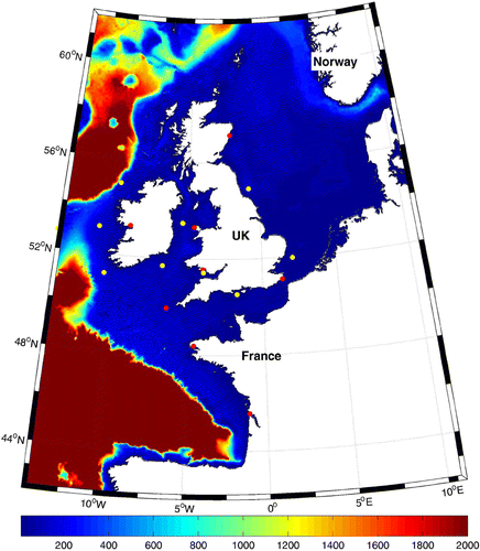
The ROMS model domain was discretised with a horizontal curvilinear grid, with a longitudinal resolution of $1/{24}^{\mathrm{o}}$ and variable latitudinal mesh size ($1/{32}^{\mathrm{o}}\sim 1/{51}^{\mathrm{o}}$ to ensure an approximately uniform cell aspect ratio. The model bathymetry was based on the ETOPO (www.ngdc.noaa.gov/mgg/global) global bathymetric data-set, which is available at a resolution of 1 arc-minute. The vertical grid consisted of 11 layers distributed according to the ROMS topographic-following coordinate system. The open boundaries of the tidal model were forced by elevation (Chapman boundary condition) and tidal velocities (Flather boundary condition), generated using 10 tidal constituents ($M_2,S_2,N_2,K_2,K_1,O_1,P_1,Q_1,M_f,M_m$) obtained from TPXO7 global tide data which has $0.{25}^{\mathrm{o}}\times 0.{25}^{\mathrm{o}}$ resolution (http://www.volkov.oce.orst.edu/tides/). The COAWST compilation switches for ROMS (cpp flags) were: SSW-BBL for combined wave–current bottom friction, WEC-VF (using vortex formalism for inclusion of wave effects on currents), horizontal and vertical mixing of momentum, and Coriolis. Regarding the turbulence closure model, Warner et al. (2005) compared different ROMS turbulence schemes which are based on the generic scale method for a number of test cases, and concluded that they lead to very similar results, apart from one scheme ($k-kl$). In the present research, we used the generic length scale closure model for turbulence modelling, set to $K-\mathit{ϵ}$ ($p=3,m=1.5$, and $n=-1$; see for details Warner et al. 2005).

Table 2. The inter-monthly variability of wave energy during 2005–2011 averaged over the NW European shelf seas (the same study area as Neill and Hashemi (2013)).

Year	Jan	Feb	Mar	Apr	May	Jun	Jul	Aug	Sep	Oct	Nov	Dec
2005	74.2	35.2	21.9	21.2	11.8	8.3	9.0	12.0	18.3	29.9	42.9	29.2
2006	32.6	37.2	29.2	20.4	15.5	8.1	9.2	8.2	17.5	24.0	67.6	84.6
2007	65.4	54.2	50.6	11.0	19.7	10.3	9.9	13.5	19.5	15.9	26.6	56.7
2008	54.1	46.1	54.5	20.9	7.2	10.2	12.0	15.0	18.7	39.5	35.1	44.9
2009	72.8	25.7	35.2	16.1	21.2	8.4	12.2	14.1	18.9	26.0	71.7	39.8
2010	30.7	31.1	25.9	18.6	9.4	10.5	17.0	9.0	19.6	32.1	50.5	25.4
2011	23.6	72.2	30.6	28.4	23.6	13.6	12.0	11.2	23.9	35.4	47.2	77.3
Avg.	50.5	43.1	35.4	19.5	15.5	9.9	11.6	11.9	19.5	29.0	48.8	51.1
SD.	21.3	15.9	12.5	5.3	6.3	1.9	2.8	2.6	2.1	7.8	16.3	22.9
Min.	23.6	25.7	21.9	11.0	7.2	8.1	9.0	8.2	17.5	15.9	26.6	25.4
Max.	74.2	72.2	54.5	28.4	23.6	13.6	17.0	15.0	23.9	39.5	71.7	84.6

Figure 2. An example of a wave field generated in the North Atlantic Ocean and approaching the UK shelf seas. The colour scale (refer to the web version) represents the significant wave height in metres. The global wave data is extracted from the ECMWF ERA-Interim dataset.

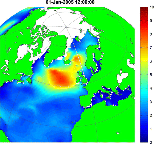
Figure 3. Validation of the ROMS results at a number of tidal gauges distributed across the domain. The absolute relative error for amplitude and phase of $M_2$ are 13 cm and $8^{\mathrm{o}}$, respectively. The corresponding values for $S_2$ amplitude and phase are 7 cm and ${11}^{\mathrm{o}}$. The locations of tidal gauges are reported in table 3.

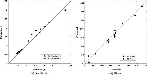
Figure 4. Comparison of the COAWST modelled amplitudes and FES2012 data. The axes units are metres.

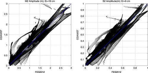
Figure 5. Cotidal charts of the main tidal constituents over the study area based on the ROMS model output. The colour scale (refer to the web version) indicates the amplitude while the phases are represented by the contour lines.

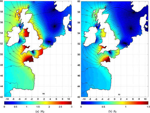
Figure 6. Tidal ellipses of the main tidal constituents representing the magnitude and direction of the tidal currents over the study area. The colour scale (refer to the web version) represents the velocity amplitude in m/s.

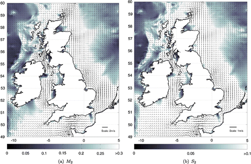
Figure 7. Validation of the COAWST wave height results at a number of wave buoys (table 3) during January 2005.

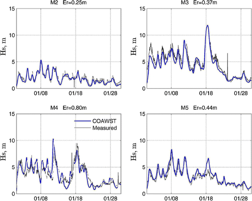
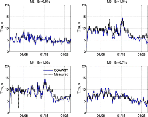
Figure 8. Validation of the COAWST wave period results at a number of wave buoys (table 3) during January 2005.

SWAN was applied to the same curvilinear grid and bathymetry as the ROMS model. However, the open boundaries for the wave model may need further treatment. Figure 2 shows a sample from the ERA-Interim data-set of a wave field generated in the North Atlantic ocean which is approaching the study area. In SWAN, it is possible to run a larger model first, and provide the boundary information for the nested model (here, the NW European shelf model; for further details see Neill and Hashemi 2013). It should be mentioned that the lower energy swell waves are a more significant component affected by the boundary forcing compared with the higher energy wind waves which are usually developed by local winds. To enhance the model performance, the wave model was nested inside a larger model of the North Atlantic Ocean. The parent model included the entire North Atlantic at a grid resolution of $1/6^{\mathrm{o}}\times 1/6^{\mathrm{o}}$, extending from ${60}^{\mathrm{o}}$W to ${15}^{\mathrm{o}}$E, and from ${40}^{\mathrm{o}}$N to ${70}^{\mathrm{o}}$N. Two-dimensional wave spectra were output hourly from the parent model and interpolated to the boundary of an inner nested model of the NW European shelf seas. Wind forcing was provided by European Centre for Medium-Range Weather Forecasts (ECMWF; www.ecmwf.int). ERA (Interim reanalysis) full resolution data, which are available three-hourly at a spatial resolution of $0.{75}^{\mathrm{o}}\times 0.{75}^{\mathrm{o}}$ were used. This wind data is based on model simulations that include data assimilation. SWAN was run in third-generation mode, with Komen linear wave growth and whitecapping, and quadruplet wave–wave interactions.

4 Results and discussion

4.1 Validation

The tide and wave results of the coupled COAWST model were first validated at a number of locations across the domain, listed in table 3. Following the validation, some results based on the coupled model are presented and discussed. Since most tidal models are forced by tidal constituents, it is a usual practice to validate model results against measured data in terms of the tidal constituents. The tidal energy of the NW European shelf seas is mainly distributed between the $M_2$ and $S_2$ components of the tide. Figure 3 shows the comparison of the model results and the measured data for these constituents. Based on these results, the relative error for amplitude and phase of $M_2$ were 13 cm and $8^{\mathrm{o}}$, respectively, which is convincing. Also, good agreement was obtained for the $S_2$ component, as shown in this figure. Additionally, model results were compared with the global FES2012 dataset (Carrère et al. 2012). This data-set is based on hydrodynamic modelling, and data assimilation of altimetry data. The mean model performance over the entire model domain was good. For instance, figure 4 shows the comparisons for $M_2$ and $S_2$ amplitudes, which led to mean absolute errors of 18 cm and 6 cm, respectively.

Cotidal maps and tidal ellipses provide a more comprehensive basis for assessment of a tidal model. The computed M2 and $S_2$ cotidal charts based on the COAWST model are plotted in figure 5. These charts show the magnitude of tidal energy in terms of tidal range over the domain. Tidal ellipses, which reflect the magnitude and direction of the tidal currents, were also computed (figure 6), and these are in convincing agreement with the results of previous model studies (e.g. Pingree and Griffiths 1979, Neill et al. 2010).

In terms of the wave results, figures 7 and 8 show validation of the COAWST model at four wave buoys within the domain (table 3) during January 2005. The model was also validated using the other wave buoys based on data provided by the Cefas WaveNet (http://www.cefasmapping.defra.gov.uk/Map) for a period of three months during 2007, as shown in figures 9 and 10. The mean absolute errors have been computed and reported for each time series. The computed errors for the wave periods and significant wave heights are about, or less than, 1 s and 0.50 m (except for the M4 buoy), respectively, which is a convincing outcome. Further, although the wind forcing was three-hourly, the model was good at predicting the peaks.

Table 3. Validation locations for COAWST tide and wave results.

Station	Coordinate
Mumbles, TG${}^{\mathrm{a}}$	3.97 W	51.57 N
St Marys, TG	6.32 W	49.93 N
Holyhead, TG	4.62 W	53.51 N
Aberdeen, TG	2.67 W	57.15 N
Dover, TG	1.32 E	51.07 N
Galway, TG	9.04 W	53.27 N
Pointe de Grave, TG	1.07 W	45.56 N
Brest, TG	4.50 W	48.38 N
M2, WB${}^{\mathrm{b}}$	5.43 W	53.48 N
M3, WB	10.55 W	51.22 N
M4, WB	9.99 W	54.99 N
M5, WB	6.70 W	51.69 N
Scarweather, WB	3.93 W	51.43 N
Poolebay, WB	1.72 W	50.63 N
West Gabbard, WB	2.08 E	51.98 N
Tynetees, WB	0.75 W	54.92 N

${}^{\mathrm{a}}$Tide Gauge ${}^{\mathrm{b}}$Wave Buoy

Figure 9. Validation of the COAWST wave height results at a number of wave buoys (table 3) during January–March 2007.

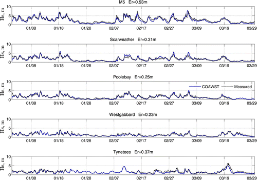
Figure 10. Validation of the COAWST wave period results at a number of wave buoys (table 3) during January–March 2007.

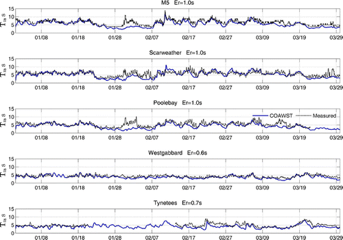
Figure 11. Comparison of the COAWST and decoupled-SWAN model performances in January 2007, at Scarweather wave buoy (table 3).

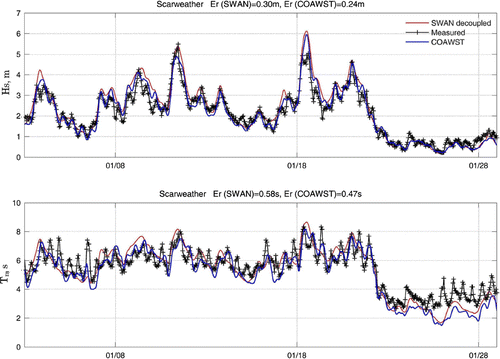
Figure 11 shows the comparison of the COAWST and decoupled-SWAN model results at Scarweather wave buoy. This wave buoy is located in the Bristol Channel (see table 3) where significant wave–current interaction effects are expected (Jones 2000). Despite the relatively coarse resolution of the grid, the modulation of the tide in the wave parameters, and improved model performances by using the COAWST model can be observed in this figure. The improvement of the model performances was 25 and 23% for the significant wave height and the mean wave period, respectively. Nevertheless, the result at a specific location can be improved by employing higher resolution models. Obviously, there will be less difference when using the coupled model at locations where the tidal currents are weaker.

4.2 Computational cost

Although coupled models tend to produce more realistic results due to the additional processes that they simulate, the computational cost of coupling can be a major drawback, discouraging their use by ocean modellers. The HPC Wales Sandy Bridge system (www.hpcwales.co.uk) was used for the simulations in the present study. The computational cost of running SWAN, ROMS and COAWST (ROMS-SWAN) are reported in table 4, which is based on the use of 2.9 GHz Sandy Bridge processors. It should be mentioned that the reported costs are approximate, and vary depending on several factors such as the number of processors which are used in each simulation. Nevertheless, they give a general indication of the computational cost associated with running the coupled model, which is about five times the cost associated with running two decoupled models. Further, as table 4 shows, nesting of the model inside a larger wave model (to enhance the model performance near the boundaries) did not change the computational cost associated with the COAWST model. However, additional time is required to run the parent SWAN model and provide the boundary information. One advantage of using the COAWST model is the ability to post-process all wave and tide data from a single (or a series of) NetCDF (Network Common Data Form) file. However, for three-hourly output data over a month of simulation, an 80 GB file was produced which, depending on the computer capacity, could be difficult to process.

4.3 Effect of waves on bed shear stress

For the first application of the coupled model, the wave induced and combined wave–current-induced average bed shear stresses are presented. As mentioned, accurate calculation of bed shear stress is essential in sediment transport and long-term morphodynamic studies. Recently, the environmental impact assessment of marine renewable energy devices has been the focus of several studies, especially in highly energetic regions of the NW European shelf seas (Neill et al. 2012). Many regions throughout this study area experience concurrently high waves and high tidal energy (e.g. Orkney in the north of Scotland; see also Neill et al. 2014). Therefore, coupled tide-wave models are useful for assessing the effect of wave energy and/or tidal energy extraction on sea-bed morphology and, in particular, the evolution of offshore sand banks (Neill et al. 2012).

Table 4. Computational cost of decoupled ROMS and SWAN compared with COAWST for one month of simulation.

Model	Number of CPUs	Simulation time, h	Total cost, CPU-h
ROMS, Decoupled	96	3.32	319
SWAN, Decoupled	96	2.81	270
COAWST (ROMS + SWAN)	96 + 96	12.01	2304
COAWST (ROMS + SWAN (Nested))	96 + 96	12.03	2310

Figure 12. Computed average and maximum wave heights during January 2005 over the domain. The colour scale (refer to the web version) shows significant wave height in metres; (a) average and (b) maximum.

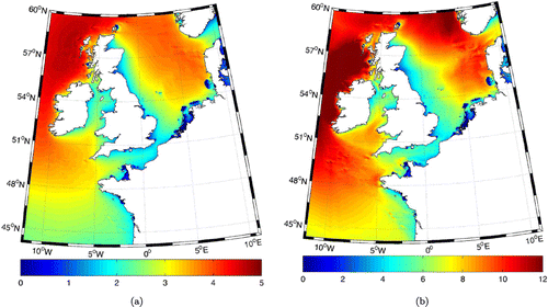
Figure 13. The average computed wave induced bottom stress (ignoring tide) and the average estimated bottom orbital velocities for January 2005 based on the COAWST results (refer to the web version for colour scales); (a) wave induced bottom stress ($\mathrm{N}/m^2$) and (b) estimated orbital velocities at the bed (m/s).

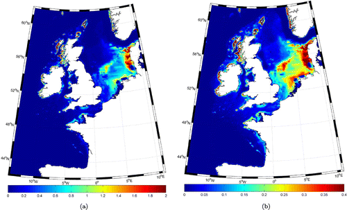
Figure 14. Average bed shear stress for January 2005, using the COAWST model for tidal current induced (ignoring waves) and combined wave-current induced cases. The colour scale (refer to the web version) is stress in $\mathrm{N}/m^2$; (a) tide induced bottom stress ($\mathrm{N}/m^2$) and (b) combined tide-wave induced bottom stress ($\mathrm{N}/m^2$).

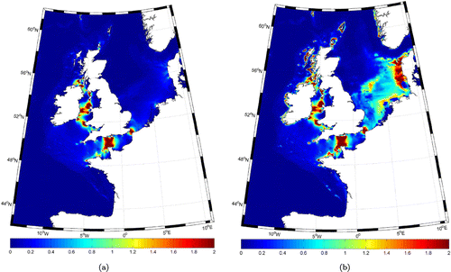
Figure 15. Effect of wave–tide interaction on the wave energy assessment for January 2005. The colour scale (refer to the web version) on the right hand plot represents the effect of tide on the wave power estimation in % which has been computed by subtracting the COAWST and decoupled SWAN model results. To avoid division by small numbers, the low-energy regions (less than 1/3 of the average) are filtered (set to green colour); (a) comparison of average wave power kW/m for January 2005, computed by different model configurations (fully coupled, one-way coupled, and uncoupled); and (b) effect of wave–tide interaction on the estimated wave power.

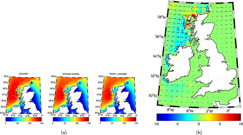
Figure 16. Effect of nesting on the computed wave parameters (refer to the web version for colour scales). The improvement of the model performance by nesting is significant, and over 30% in the west coasts of Ireland and Scotland. The effect is negligible in many parts of the Irish Sea and North Sea; (a) average wave power in January 2005 (left; kW/m) and effect of nesting on the results (right; %); and (b) effect of nesting on mode results at M3 wave buoy (see sub-figure a for location) in January 2005.

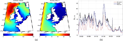
Figure 12 shows the mean and peak wave height over the model domain during January 2005. The average and maximum computed wave heights follow a similar spatial pattern. The most energetic regions are NW of Scotland and west of Ireland as opposed to the more sheltered east coast of the UK, central parts of the Irish Sea and the English Channel.

The wave orbital velocity, estimated near the bed, is the basis for computation of the wave induced bed shear stresses and can be directly output from SWAN. Alternatively, it can be computed using the following equation,10 $$\begin{array}{c}\hfill u_b=\frac{\mathit{\pi }{H}_s}{T_{w}sinh(kd)},\end{array}$$10 where T_w is the wave period, H_s is the significant wave height and d is the water depth. Figure 13 shows the average wave induced bed shear stress, and the corresponding near-bed orbital velocities over the domain. As expected, exposed shallow regions are associated with higher wave induced bed shear stresses. In particular, western coasts of Scotland and Ireland, and the western coast of Denmark, are more affected by wave-induced bed shear stresses. Also, figure 14 shows the tide induced and combined wave–tide induced bed shear stresses over the domain. The spatial pattern of more active sediment transport regions based on the combined wave–tide effect can be inferred from this figure. It should be mentioned that the nearshore physics of the COAWST model, which includes wave breaking and surf zone parameterisation of wave–current interactions cannot be implemented in models at this scale and resolution. Therefore, regional models with higher grid resolution are necessary for detailed assessment of the bed shear stress, and the resulting sediment transport for a particular case study.

4.4 Effect of tides on wave energy assessment

As a second application, the effect of tides on wave energy assessment is presented here. In the majority of previous research on the assessment of wave energy over the NW European shelf seas, the effect of tides has not been included (e.g. the Atlas of UK marine renewable energy resources ABPmer 2008). There are two ways to include the effect of tides on the wave resource using SWAN. The first method (Hashemi and Neill 2014), which needs much less computational effort, is providing wave and current data files extracted from a ROMS simulation as input files for SWAN and running the decoupled SWAN model (one-way coupling). The other method, which is more expensive, is to estimate the wave power by the fully coupled COAWST model. The advantage of the latter method lies in its flexibility and its more complete analysis of wave–current interaction, particularly when two-way interaction is important. Figure 15 shows the results for the three modelling approaches used to estimate the average wave energy resource for the most energetic part of the domain, and the effect of wave–tide interactions. As figure 15(a) shows, the decoupled SWAN model, one-way coupled model, and the COAWST model seem to produce very similar results. However, the wave–tide interaction effect becomes clearer when the differences between the model results are plotted. Referring to figure 15(b), although the impact is not significant when expressed as a percentage over the whole domain, in some specific regions (e.g. Orkney) it can reach 10% of the resource. Since the effect has been plotted as a percentage of the resource, only the regions with significant wave resources (higher than 1/3 of the average; to avoid division by small numbers) have been plotted. Further, the dominant wave climate of this region is southwesterly (Neill and Hashemi 2013), but the dominant waves for the simulation period were westerly. The temporal and spatial variability of this effect needs further research.

Figure 16 demonstrates how model performance and wave resource estimation are affected by the western boundary of the domain. Figure 16(b) shows the significant improvement of the model results for an exposed wave buoy which is relatively close to the boundary. Additionally, it can be concluded from figure 16(a) that in many potential wave energy development sites (e.g. Scotland), more than 30% of the wave energy resources are generated outside the region (i.e. swell waves), during the simulation period.

5 Conclusions

A COAWST coupled tide-wave model of the NW European shelf seas has been developed, and some applications of the model discussed. While the COAWST model can theoretically implement many wave-tide interaction processes, the application of the model for shelf scale simulations is highly constrained by computational costs (about five times the cost of decoupled simulations) and model resolution. The flexibility of the model, which allows the user to switch on/off a particular physical process, is a major advantage for this model. However, in large-scale applications of the model, the main challenge for the user is the selection of the appropriate model physics, through cpp switches, that are applicable over the entire domain. This becomes even more complicated when one tries to develop a model with a minimum number of physical processes for simplicity, and in order to reduce the computational cost for large scale simulations where in some parts of a region one physical process is dominant (e.g. wave induced stresses) as opposed to other regions (e.g. baroclinic currents). Further, although the computational cost of running the decoupled SWAN, using current and water elevation data provided by ROMS simulations (one-way coupling), is significantly less than that of the COAWST model, the pre/post-processing of the input and output data is much more convenient in COAWST, which reduces the user time and the corresponding cost.

The performance of the COAWST model in prediction of wave parameters was shown to improve by 25% in places where wave–current interaction is significant.

Application of the model in estimating the combined wave–tide-induced bed shear stress over the study area shows importance of the waves in sediment transport processes at shelf sea scale, and is consistent with the results of previous research. Application of the model in the assessment of wave energy resources has demonstrated the significance of tides in wave resource assessment which in some regions can alter the estimated wave power by more than 10%. For accurate wave studies, the COAWST model of the NW European shelf seas should be nested inside a larger model covering the North Atlantic to account for swell waves which have been generated outside the domain. This effect exceeded 30% in many potential wave energy sites exposed to North Atlantic Ocean, for the selected period.

Acknowledgements

The authors thank the European Centre for Medium-Range Weather Forecasting (ECMWF) for supplying the wind and some wave model data, and also NOAA for providing the ETOPO bathymetric data. The wave buoy data used for model validation was supplied by the Irish Marine Institute, BODC, and Cefas WaveNet. The model simulations were made on High-Performance Computing (HPC) Wales, a collaboration between Welsh universities, the Welsh Government, and Fujitsu. This work was undertaken as part of the SEACAMS project, which is part-funded by the European Union’s Convergence European Regional Development Fund, administered by the Welsh Government. Simon P. Neill acknowledges the support of EPSRC SuperGen project EP/J010200/1. The authors also gratefully acknowledge the UK National Oceanography Centre for its support in publishing the present research.

References

- ABPmer, The Met Office and Proudman Oceanographic Laboratory; Atlas of UK marine renewable energy resources. Technical report, Department for Business Enterprise & Regulatory Reform, 2008.
- Barbariol, F., Benetazzo, A., Carniel, S. and Sclavo, M., Improving the assessment of wave energy resources by means of coupled wave-ocean numerical modeling. Renew. Energ. 2013, 60, 462–471.
- Benetazzo, A., Carniel, S., Sclavo, M. and Bergamasco, A., Wave-current interaction: effect on the wave field in a semi-enclosed basin. Ocean Model. 2013, 70, 152–165.
- Bolanos, R., Osuna, P., Wolf, J., Monbaliu, J. and Sanchez-Arcilla, A., Development of the POLCOMS-WAM current-wave model. Ocean Model. 2011, 36, 102–115.
- Bolanos-Sanchez, R., Wolf, J., Brown, J., Osuna, P., Monbaliu, J. and Sanchez-Arcilla, A., Comparison of wave-current interaction formulation using POLCOMS-WAM wave-current model, in Proceedings of the 31st International Conference on Coastal Engineering, Hamburg, Germany, 2009.
- Brown, J.M., Souza, A.J. and Wolf, J., An 11-year validation of wave-surge modelling in the Irish Sea, using a nested POLCOMS-WAM modelling system. Ocean Model. 2010, 33, 118–128.
- Carrère, L., Lyard, F., Cancet, M., Guillot, A. and Roblou, L., FES2012: a new global tidal model taking advantage of nearly 20 years of altimetry, in Proceedings of meeting, 20 years of altimetry, Venice-Lido, Italy, 2012.
- Davies, A., Soulsby, R. and King, H., A numerical model of the combined wave and current bottom boundary layer. J. Geophys. Res.-Oceans 1988, 93, 491–508.
- Di Lorenzo, E., Moore, A.M., Arango, H.G., Cornuelle, B.D., Miller, A.J., Powell, B., Chua, B.S. and Bennett, A.F., Weak and strong constraint data assimilation in the inverse regional ocean modeling system (ROMS): development and application for a baroclinic coastal upwelling system. Ocean Model. 2007, 16, 160–187.
- Egbert, G.D. and Ray, R.D., Semi-diurnal and diurnal tidal dissipation from TOPEX/Poseidon altimetry. Geophys. Res. Lett. 2003, 30, 1907, 9-1–9-4. doi:10.1029/2003GL017676.
- Haidvogel, D.B., Arango, H., Budgell, W.P., Cornuelle, B.D., Curchitser, E., Di Lorenzo, E., Fennel, K., Geyer, W.R., Hermann, A.J., Lanerolle, L., Miller, A.J., Moore, A.M., Powell, T.M., Shchepetkin, A.F., Sherwood, C.R., Signell, R.P., Warner, J.C. and Wilkin, J., Ocean forecasting in terrain-following coordinates: Formulation and skill assessment of the Regional Ocean Modeling System. J. Comput. Phys. 2008, 227, 3595–3624.
- Hashemi, M.R. and Neill, S.P., The role of tides in shelf-scale simulations of the wave energy resource. Renew. Energ. 2014, 69, 300–310.
- Jones, B., A numerical study of wave refraction in shallow tidal waters. Estuar. Coast. Shelf Sci. 2000, 51, 331–347.
- Kumar, N., Voulgaris, G., Warner, J.C. and Olabarrieta, M., Implementation of the vortex force formalism in the coupled ocean-atmosphere-wave-sediment transport (COAWST) modeling system for inner shelf and surf zone applications. Ocean Model. 2012, 47, 65–95.
- MacCready, P., Banas, N.S., Hickey, B.M., Dever, E.P. and Liu, Y., A model study of tide-and wind-induced mixing in the Columbia River estuary and plume. Cont. Shelf Res. 2009, 29, 278–291.
- Madsen, O.S., Spectral wave-current bottom boundary layer flows. Coastal Eng. Proc. 1994, 1, 384–398.
- Malarkey, J. and Davies, A.G., A non-iterative procedure for the Wiberg and Harris (1994) oscillatory sand ripple predictor. J. Coast. Res. 2003, 19, 738–739.
- Mellor, G.L., The depth-dependent current and wave interaction equations: a revision. J. Phy. Oceanogr. 2008, 38, 2587–2596.
- Neill, S.P. and Hashemi, M.R., Wave power variability over the northwest European shelf seas. App. Energ. 2013, 106, 31–46.
- Neill, S.P., Hashemi, M.R. and Lewis, M.J., The role of tidal asymmetry in characterizing the tidal energy resource of Orkney. Renew. Energ. 2014, 68, 337–350.
- Neill, S.P., Jordan, J.R. and Couch, S.J., Impact of tidal energy converter (TEC) arrays on the dynamics of headland sand banks. Renew. Energ. 2012, 37, 387–397.
- Neill, S.P., Scourse, J.D. and Uehara, K., Evolution of bed shear stress distribution over the northwest European shelf seas during the last 12,000 years. Ocean Dynam. 2010, 60, 1139–1156.
- Newberger, P. and Allen, J.S., Forcing a three-dimensional, hydrostatic, primitive-equation model for application in the surf zone: 1. Formulation. J. Geophys. Res.- Oceans 2007a, 112, C08018 1–12.
- Newberger, P. and Allen, J.S., Forcing a three-dimensional, hydrostatic, primitive-equation model for application in the surf zone: 2. Application to DUCK94. J. Geophys. Res.- Oceans 2007b, 112, C08019 1–21.
- Pingree, R. and Griffiths, D., Sand transport paths around the British Isles resulting from M2 and M4 tidal interactions. J. Mar. Biol. Assoc. UK 1979, 59, 497–513.
- Reniers, A., Thornton, E., Stanton, T. and Roelvink, J., Vertical flow structure during Sandy Duck: observations and modeling. Coast. Eng. 2004, 51, 237–260.
- Saruwatari, A., Ingram, D.M. and Cradden, L., Wave-current interaction effects on marine energy converters. Ocean Eng. 2013, 73, 106–118.
- Soulsby, R. and Clarke, S., Bed shear-stresses under combined waves and currents on smooth and rough beds. HR Wallingford, Report TR137, 2005.
- Styles, R. and Glenn, S.M., Modeling bottom roughness in the presence of wave-generated ripples. J. Geophys. Res.-Oceans 2002, 107, 3110, 24-1-–24-15.
- Tolman, H., An evaluation of expressions for wave energy dissipation due to bottom friction in the presence of currents. Coast. Eng. 1992, 16, 165–179.
- Uchiyama, Y., McWilliams, J.C. and Shchepetkin, A.F., Wave-current interaction in an oceanic circulation model with a vortex-force formalism: Application to the surf zone. Ocean Model. 2010, 34, 16–35.
- Warner, J.C., Armstrong, B., He, R. and Zambon, J.B., Development of a coupled ocean-atmosphere-wave-sediment transport (COAWST) modeling system. Ocean Model. 2010, 35, 230–244.
- Warner, J.C., Sherwood, C.R., Arango, H.G. and Signell, R.P., Performance of four turbulence closure models implemented using a generic length scale method. Ocean Model. 2005, 8, 81–113.
- Warner, J.C., Sherwood, C.R., Signell, R.P., Harris, C.K. and Arango, H.G., Development of a three-dimensional, regional, coupled wave, current, and sediment-transport model. Comput. Geosci. 2008, 34, 1284–1306.
- Wolf, J., Coastal flooding: impacts of coupled wave-surge-tide models. Nat. Hazards 2009, 49, 241–260.