The dynamics of waves interacting with the Equatorial Undercurrent

Abstract

We propose a new, simple model – but one which has far-reaching consequences – to describe the interaction between waves that propagate across the Pacific Ocean and the Equatorial Undercurrent (EUC). This involves a detailed discussion of the full linear problem as it relates to the dynamic coupling between the surface waves and the internal waves on the thermocline. The result is a comprehensive description of the system close to the Equator, and how the structure of the EUC affects the wave properties; in particular, the analysis holds for arbitrary wavelengths and finite depths. Although the final expressions, for general wavelengths, are too cumbersome for direct interpretation, we are able to produce simple formulae for the speeds of the waves, and the attenuation factor between the two families of waves, for short, intermediate and long waves. Further, our results predict the appearance of critical layers under certain circumstances; by reverting to our original system of governing equations, we are able to derive the relevant nonlinear structure of the flow in these layers. Our results are in good agreement with the available field data.

Keywords:

• Ocean waves
• Wind-drift current
• Equatorial Undercurrent
• Dispersion relation
• Wave coupling

1. Introduction

The dynamics of the Pacific Ocean, within a band about $2^{\circ }$ latitude from the Equator, comprises a rich variety of phenomena, which is due to the interplay between several factors, the most significant being:

(i)	The pronounced stratification in this equatorial region, greater than anywhere else in the ocean (see Fedorov and Brown 2009). This is exemplified by the presence of a sharp, near-surface pycnocline/thermocline which separates a shallow layer of relatively warm water (and so less dense) near the surface, from a deeper layer of denser, colder water. The difference in density across the thermocline is about $1\%$, and it is a reasonable assumption to represent the stratification as a shallow sub-surface layer of constant density ${\overline{\mathit{\rho }}}_0$, overlying a deep layer of constant density $(1+r){\overline{\mathit{\rho }}}_0$, where $r$ is a small positive constant (see McCreary 1985).
(ii)	The presence of underlying non-uniform currents (see McCreary 1985, Proehl et al. 1986). More precisely, in a band approximately 300 km wide about the Equator, the underlying currents are highly depth-dependent: in a sub-surface layer, typically extending no more than about 100 m down, there is a westward drift that is driven by the prevailing trade winds; just below this there lies the Equatorial Undercurrent (EUC), an eastward jet whose core resides on the thermocline. Below the EUC, the motion dies out rapidly so that, at depths in excess of about 240 m, we have an abyssal layer of essentially still water.
(iii)	Many types of ocean flows in this region, due to the wide variety of wave motions that are possible (and observed). The importance of long waves, with wavelengths exceeding 100 km, is well-documented (see Fedorov and Brown 2009) and there is ample evidence of large-amplitude internal waves, these having relatively short wavelengths (typically a few hundreds of metres) and periods about 5–10 min (see Moum et al. 2011).

The usual approach, leading to some insight into the dynamics of this oceanic system, is based on reduced-gravity, shallow-water, linear theory, assuming an ocean of infinite depth and a motionless layer below the thermocline (McCreary 1985); in addition, only wavelengths greatly in excess of the mean depth of the thermocline are considered (Fedorov and Brown 2009). This choice of model has two distinct drawbacks: the shorter waves are filtered out and, more significantly, flows with a more elaborate vertical structure are ignored. This assumption that the equatorial current field is passive (in so far as it affects the properties and response of the waves) is a serious impediment to the usefulness of any results. Indeed, the EUC, despite being a narrow and near-surface current (its core at depths of 100–200 m, about 80 m thick and about 200 km wide), is an appreciable flow which traverses the entire length of the Pacific Ocean at the Equator (about 13000 km), attaining speeds of about 1 ms${}^{-1}$. Although discovered in the 19th Century, the EUC was essentially forgotten until it was rediscovered in 1952 (see Philander 1980). The presence of the EUC, and of the westward wind-driven drift near the surface, have profound effects on the equatorial waves and these, in turn, are key factors in more general ocean dynamics: they induce motions of the thermocline. In particular, the equatorial-current field is altered during the occurrence of the El Niño phenomenon. (This was so-named – it is Spanish for “The Christ Child” – by Peruvian fishermen in the 19th Century, to describe the warm current that appeared each year, about Christmas time, in the coastal waters off western South America.) The effect is driven by the weakened trade winds which then allow an abnormally high eastward flow of warm water; nowadays, El Niño usually refers to irregular, strong events of this type.

There have been studies that address the problem of the interaction of the equatorial waves with an oceanic mean flow; these have evolved along two relatively distinct lines. The main thrust of these investigations, initiated by McPhaden et al. (1986) and Proehl et al. (1986), specifies a background state that captures the structure of the equatorial current field, and then assumes that the dynamics for its perturbation is linear, hydrostatic and Boussinesq. In its favour is the fact that this approach can allow for the presence of critical levels, i.e. where the wave speed equals the mean-flow speed at some depth, a property that is not within the reach of existing reduced-gravity, shallow-water models. The importance of the existence of these critical levels is that they are at the heart of the mechanisms that trigger instabilities within the flow (see Maslowe 1986). Indeed, subthermoclinic eddies, associated with critical layers, have been reported by Chiang and Qu (2013). However, McPhaden et al. (1986) and Proehl et al. (1986) do not develop an in-depth perturbative analysis; these authors resort to a numerical treatment of their system by means of finite differences. The disadvantage of seeking numerical solutions, without an underlying solution-structure, is the difficulty, often encountered, of being able to identify clearly the important processes that are at work. An alternative approach – the other line of investigation – is to seek explicit solutions to the nonlinear governing equations, the advantage being that these provide a way of studying, in detail, specific aspects of the whole flow system, without recourse to approximations of any sort. Recently, explicit nonlinear solutions were obtained in the Lagrangian framework, these being for equatorially-trapped waves (see Constantin 2012, Henry 2013). Correspondingly, solutions for the internal waves have been described in Constantin (2014). However, both these types of solution are restricted to relatively short wavelengths, and they are realistic representations of the flow only for the region near the surface and in the neighbourhood of the thermocline, respectively. The main reason for these solutions’ inability to cope satisfactorily with the entire vertical extent of the equatorial flow is down to the limitations on the permissible underlying currents – the methods cannot admit realistic equatorial current fields; furthermore, the approach adopted avoids any possibility of the appearance of critical levels.

The aim of this paper is to attempt to rectify some of the shortcomings in the earlier work. In particular, we will develop an in-depth analysis of the two-dimensional linear problem, based on a simple model for the equatorial wave-current interaction that accommodates all the salient features of the current field in the Pacific Ocean near the Equator. Because our main interest is in the interaction of waves with the EUC, and this has an overall meridional extent of about 200 km, we invoke the $f$-plane approximation. It is not our intention to investigate the flows at higher latitudes, where the $f$-plane approximation breaks down. Indeed, at these latitudes, there are other strong sub-surface currents that lead to a significant increase in the complexity of the system and, correspondingly, to the models that we might employ. Further, we will not address the effects of a variable bottom-topography.

Our approach enables us to study the coupling between the waves at the surface and those on the thermocline, and how both these wave systems interact with the background flow. The waves will propagate in a longitudinal direction, in a flow with a vanishing meridional velocity component; we do not investigate the dynamics close to the eastern and western boundaries of the ocean basin. The background flow, which will model the wind-driven, westerly near-surface flow and the easterly EUC, is chosen to be a profile with a piecewise constant vorticity. Indeed, it is this choice which makes it possible to analyse the problem completely and in detail: the mathematical problem in the case of constant vorticity is very little different from the irrotational case. We develop the solution of the linear problem, for arbitrary wavelength, although the results turn out to be rather cumbersome, in general. Nevertheless, we are readily able to extract simple, and illuminating, results by examining different regimes: short waves; intermediate waves (long with respect to the depth of the thermocline, but not with respect to the depth of the ocean); long waves (with respect to the depth of the ocean). We present approximations for the wave speeds, and the strength of the coupling between the two families of waves, in all three cases, and test our results against the available data. The strength of this approach, as compared to numerical simulations (current or future), is the inclusion of many different wavelength regimes within the one model, and the opportunity to identify the important factors that control the flow e.g. the density difference, the depth of the EUC, the thickness of the core of the EUC, and so on. Any numerical exercise that could encompass all this would be, in all likelihood, so excessive as to preclude it as a worthwhile undertaking. While most of our presentation here will be devoted to a detailed discussion of the linear problem, our approach enables us to develop directly the appropriate nonlinear analysis for the inclusion of critical layers, as they appear – and they do. In the absence of viscosity in our model, we must invoke a nonlinear mechanism for the description of the flow in the neighbourhood of a critical layer: a corresponding viscous structure is not available to us, via our choice of the Euler equation as our fundamental governing equation. Indeed, in conventional geophysical-fluid-dynamical considerations, the Reynolds number is extremely large (see Maslowe 1986), and so the use of nonlinearity is advisable.

The plan, in this paper, is: in section 2, to present the governing equations and boundary conditions, to introduce a suitable non-dimensionalisation and to define the background flow that we choose to use here; in section 3, to describe the general solution of the linear problem; in section 4, to give the details for short waves, then (section 5) for intermediate waves and long waves. A discussion and conclusions are to be found in section 6. We also provide a number of appendices that cover more technical aspects of some of the work, including an introduction to the theory of critical layers as they apply in this scenario.

2. Preliminaries

We present the governing equations that provide the simplest description that captures the relevant dynamics, together with an appropriate non-dimensionalisation of them. We also introduce the model that we use for the background flow, which accommodates the essential features that we have discussed above.

2.1. The f-plane approximation

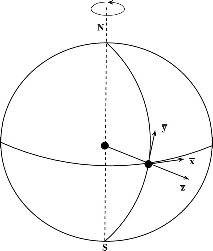
For oceanic motions of a limited meridional extent, within $2^{\circ }$ from the Equator, it is adequate to use the $f$-plane approximation in the governing equations, as discussed by LeBlond and Mysak (1978). We adopt a coordinate system with the origin at a point on the Earth’s surface, with the $\overline{x}$-axis chosen horizontally due East, the $\overline{y}$-axis horizontally due North (in the tangent plane) and the $\overline{z}$-axis upward (see figure 1).

Figure 1. The rotating frame of reference, with the $\overline{x}$-axis chosen horizontally due East, the $\overline{y}$-axis horizontally due North and the $\overline{z}$-axis upward.

Let $\overline{\mathfrak{u}}$, $\overline{\mathfrak{v}}$, $\overline{\mathfrak{w}}$, denote the corresponding fluid velocity components in the direction of increasing azimuth, latitude and elevation, respectively, where we have used the over-bar to represent the physical variables; this notation will be simplified shortly. If $\overline{\mathit{\Omega }}$ is the (constant) rotational speed of the Earth round the polar axis toward the East, having the approximate magnitude $7.29\times {10}^{-5}$ rad s${}^{-1}$, $\overline{t}$ stands for time, $\overline{g}\approx 9.8$ ms${}^{-2}$ is the (constant) gravitational acceleration at the Earth’s surface, $\overline{\mathit{\rho }}$ is the water density, and $\overline{\mathfrak{P}}$ is the pressure, the governing equations for ocean waves are the suitably adjusted Euler equations(1a) $$\begin{array}{cc}\hfill {\overline{\mathfrak{u}}}_{\overline{t}}+\overline{\mathfrak{u}}{\overline{\mathfrak{u}}}_{\overline{x}}+\overline{\mathfrak{v}}{\overline{\mathfrak{u}}}_{\overline{y}}+\overline{\mathfrak{w}}{\overline{\mathfrak{u}}}_{\overline{z}}+2\overline{\mathit{\Omega }}\overline{\mathfrak{w}}& {\displaystyle =-\frac{1}{\overline{\mathit{\rho }}}{\overline{\mathfrak{P}}}_{\overline{x}},}\hfill \end{array}$$(1a) (1b) $$\begin{array}{cc}\hfill {\overline{\mathfrak{v}}}_{\overline{t}}+\overline{\mathfrak{u}}{\overline{\mathfrak{v}}}_{\overline{x}}+\overline{\mathfrak{v}}{\overline{\mathfrak{v}}}_{\overline{y}}+\overline{\mathfrak{w}}{\overline{\mathfrak{v}}}_{\overline{z}}& {\displaystyle =-\frac{1}{\overline{\mathit{\rho }}}{\overline{\mathfrak{P}}}_{\overline{y}},}\hfill \end{array}$$(1b) (1c) $$\begin{array}{cc}\hfill {\overline{\mathfrak{w}}}_{\overline{t}}+\overline{\mathfrak{u}}{\overline{\mathfrak{w}}}_{\overline{x}}+\overline{\mathfrak{v}}{\overline{\mathfrak{w}}}_{\overline{y}}+\overline{\mathfrak{w}}{\overline{\mathfrak{w}}}_{\overline{z}}-2\overline{\mathit{\Omega }}\overline{\mathfrak{u}}& {\displaystyle =-\frac{1}{\overline{\mathit{\rho }}}{\overline{\mathfrak{P}}}_{\overline{z}}-\overline{g},}\hfill \end{array}$$(1c) and the equation of mass conservation(2) $$\begin{array}{c}\hfill {\overline{\mathit{\rho }}}_{\overline{t}}+\overline{\mathfrak{u}}{\overline{\mathit{\rho }}}_{\overline{x}}+\overline{\mathfrak{v}}{\overline{\mathit{\rho }}}_{\overline{y}}+\overline{\mathfrak{w}}{\overline{\mathit{\rho }}}_{\overline{z}}=0,\end{array}$$(2)

together with the condition of incompressibility(3) $$\begin{array}{c}\hfill {\overline{\mathfrak{u}}}_{\overline{x}}+{\overline{\mathfrak{v}}}_{\overline{y}}+{\overline{\mathfrak{w}}}_{\overline{z}}=0\end{array}$$(3)

throughout the fluid. To justify the use of the $f$-plane approximation, note that half of the Earth lies at latitudes of less than ${30}^{\circ }$ and in these regions, when the spatial scale of an ocean-atmosphere motion is of the order of 1000 km, then the use of the $\mathit{\beta }$-plane approximation is appropriate; see the discussions in Gill (1982) and Majda and Wang (2006). This approximation stems from a Taylor expansion of the components of the Coriolis force$$2\overline{\mathit{\Omega }}\left(\begin{array}{c}\overline{\mathfrak{w}}cos(\overline{y}/R)-\overline{\mathfrak{v}}sin(\overline{y}/R)\\ \overline{\mathfrak{u}}sin(\overline{y}/R)\\ -\overline{\mathfrak{u}}cos(\overline{y}/R)\end{array}\right),$$

near the reference latitude, so $cos(\overline{y}/R)\approx 1$ and $sin(\overline{y}/R)\approx \overline{y}/R$ near the Equator, where $R\approx 6378$ km is the equatorial radius of the Earth. The $f$-plane approximation retains only the first (i.e. constant) term of the expansion, while the inclusion of the term $\mathit{\beta }\overline{y}$, with $\mathit{\beta }=2\overline{\mathit{\Omega }}/R\approx 2.28\times {10}^{-11}{\text{m}}^{-1}{\text{s}}^{-1}$, in the $\mathit{\beta }$-plane approximation, allows for the effects of meridional variation (cf. Gerkema et al. 2004). That is, in the equatorial $\mathit{\beta }$-plane approximation, we have to replace (1) by(4a) $$\begin{array}{cc}\hfill {\overline{\mathfrak{u}}}_{\overline{t}}+\overline{\mathfrak{u}}{\overline{\mathfrak{u}}}_{\overline{x}}+\overline{\mathfrak{v}}{\overline{\mathfrak{u}}}_{\overline{y}}+\overline{\mathfrak{w}}{\overline{\mathfrak{u}}}_{\overline{z}}+2\overline{\mathit{\Omega }}\overline{\mathfrak{w}}-\mathit{\beta }\overline{y}\overline{\mathfrak{v}}& {\displaystyle =-\frac{1}{\overline{\mathit{\rho }}}{\overline{\mathfrak{P}}}_{\overline{x}},}\hfill \end{array}$$(4a) (4b) $$\begin{array}{cc}\hfill {\overline{\mathfrak{v}}}_{\overline{t}}+\overline{\mathfrak{u}}{\overline{\mathfrak{v}}}_{\overline{x}}+\overline{\mathfrak{v}}{\overline{\mathfrak{v}}}_{\overline{y}}+\overline{\mathfrak{w}}{\overline{\mathfrak{v}}}_{\overline{z}}+\mathit{\beta }\overline{y}\overline{\mathfrak{u}}& {\displaystyle =-\frac{1}{\overline{\mathit{\rho }}}{\overline{\mathfrak{P}}}_{\overline{y}},}\hfill \end{array}$$(4b) (4c) $$\begin{array}{cc}\hfill {\overline{\mathfrak{w}}}_{\overline{t}}+\overline{\mathfrak{u}}{\overline{\mathfrak{w}}}_{\overline{x}}+\overline{\mathfrak{v}}{\overline{\mathfrak{w}}}_{\overline{y}}+\overline{\mathfrak{w}}{\overline{\mathfrak{w}}}_{\overline{z}}-2\overline{\mathit{\Omega }}\overline{\mathfrak{u}}& {\displaystyle =-\frac{1}{\overline{\mathit{\rho }}}{\overline{\mathfrak{P}}}_{\overline{z}}-\overline{g}.}\hfill \end{array}$$(4c) The problem that we must now address is how we might reasonably simplify the system (4) further, even after the introduction of the $\mathit{\beta }$-plane approximation. In this first attempt to produce a fairly general and mathematically coherent description of the wave perturbation of a realistic model for the background flow, we aim to capture many – but not all – the essential characteristics of the flow in a suitable neighbourhood of the Equator. To this end, we are driven to limit ourselves to a two-dimensional configuration, but we shall retain many other physical properties of the flow in our attempt to explain many of the phenomena that are observed. In order to make headway, we therefore choose to work with a model in which any meridional motion is absent; correspondingly, there is no variation in the meridional direction, i.e. $\overline{\mathfrak{v}}\equiv 0$ and $\mathit{\partial }/\mathit{\partial }\overline{y}\equiv 0$. Observations given by Johnson and McPhaden (2001) show that meridional speeds near the Equator are much smaller than the zonal speeds. However, it is known that, in some circumstances, the amplitudes of the eddy perturbations can be roughly the same size in all three directions and, occasionally, larger than the mean flow. We cannot, at this stage of our investigations, include this more complicated scenario. Further, the absence of any dependence on $\overline{y}$ also implies that we must limit ourselves, at most, to the $f$-plane approximation. The form of the relevant Coriolis terms in (4), written using our non-dimensional scheme, described in (19(19) $$\begin{array}{cc}\hfill \overline{z}& =\overline{h}z,\overline{x}=\overline{h}x,\overline{t}=\overline{h}t/\sqrt{\overline{g}\overline{h}},\overline{\mathit{\eta }}=\overline{a}\mathit{\eta },\overline{H}=\overline{a}H,\hfill \\ \hfill (\overline{U}+\overline{u},\overline{w})& =\sqrt{\overline{g}\overline{h}}(U+u,w),\overline{P}+\overline{p}=\overline{{\mathit{\rho }}_0}\overline{g}\overline{h}(P+p),\hfill \end{array}$$(19) ) below, become$$\begin{array}{c}x-\text{momentum equation}:2\mathit{\Omega }(w-{\displaystyle \frac{yv}{\widehat{R}}}),\hfill \\ y-\text{momentum equation}:{\displaystyle \frac{2\mathit{\Omega }}{\widehat{R}}}yu,\hfill \\ z-\text{momentum equation}:-2\mathit{\Omega }u,\hfill \end{array}$$

where the parameters are $\mathit{\Omega }=\overline{\mathit{\Omega }}\overline{h}/\sqrt{\overline{g}\overline{h}}$ and $\widehat{R}=R/\overline{h}$; here $\overline{h}$ is the mean depth of the thermocline. These parameters take values of approximately $\mathit{\Omega }\approx 2.5\times {10}^{-4}$ and ${\widehat{R}}^{-1}\approx 2\times {10}^{-5}$ for the EUC. On this basis we may therefore define the mathematical problem as that with $\widehat{R}\to \infty$, in conjunction with the two-dimensionality assumption. This procedure retains the terms in $\mathit{\Omega }$ (but not in $\mathit{\Omega }/\widehat{R}$), which corresponds to the $f$-plane approximation. This, in turn, means that we shall still be able to identify the dominant effects of the Coriolis force, even if the associated coefficient is numerically very small – indeed, we can take advantage of this small size when we provide some estimates later.

In summary, therefore, we must limit the applicability of our theory to regions quite close to the Equator (at least 50 km, but some authors work with as much as 150 km, either side), and to flows which can be regarded as approximately two dimensional. Even with these restrictions, we suggest that the applicability of our quite detailed theory will help us to understand important features of the equatorial ocean dynamics.

2.2. The governing equations

We take as our governing equations the Euler equation, suitably adjusted for the $f$-plane, together with the corresponding equation for an incompressible fluid (although with different, constant densities above and below the thermocline), and with no meridional flow variations; in particular, we assume a vanishing meridional velocity component. The equations are therefore(5a) $$\begin{array}{cc}\hfill {\overline{\mathfrak{u}}}_{\overline{t}}+\overline{\mathfrak{u}}{\overline{\mathfrak{u}}}_{\overline{x}}+\overline{\mathfrak{w}}{\overline{\mathfrak{u}}}_{\overline{z}}+2\overline{\mathit{\Omega }}\overline{\mathfrak{w}}& {\displaystyle =-\frac{1}{\overline{\mathit{\rho }}}{\overline{\mathfrak{P}}}_{\overline{x}},}\hfill \end{array}$$(5a) (5b) $$\begin{array}{cc}\hfill {\overline{\mathfrak{w}}}_{\overline{t}}+\overline{\mathfrak{u}}{\overline{\mathfrak{w}}}_{\overline{x}}+\overline{\mathfrak{w}}{\overline{\mathfrak{w}}}_{\overline{z}}-2\overline{\mathit{\Omega }}\overline{\mathfrak{u}}& {\displaystyle =-\frac{1}{\overline{\mathit{\rho }}}{\overline{\mathfrak{P}}}_{\overline{z}}-\overline{g},}\hfill \end{array}$$(5b) (6) $$\begin{array}{c}\hfill {\overline{\mathfrak{u}}}_{\overline{x}}+{\overline{\mathfrak{w}}}_{\overline{z}}=0.\end{array}$$(6)

The density $\overline{\mathit{\rho }}$ of the fluid is a constant $\overline{{\mathit{\rho }}_0}$ above the thermocline (at $\overline{z}=-\overline{h}+\overline{H}(\overline{x},\overline{t})$), of mean depth $\overline{h}$, and is replaced by $\overline{{\mathit{\rho }}_0}(1+r)$ for the fluid below the thermocline, where $r$ is a small positive constant; typically $r$ lies in the range from $4\times {10}^{-3}$ to $6\times {10}^{-3}$ (cf. Kessler and McPhaden 1995, Fedorov and Brown 2009). The appropriate boundary conditions are, at the free surface $\overline{z}=\overline{\mathit{\eta }}(\overline{x},\overline{t})$, the dynamic boundary condition(7) $$\begin{array}{c}\hfill \overline{\mathfrak{P}}={\overline{P}}_{\mathrm{a}tm}\text{on}\overline{z}=\overline{\mathit{\eta }}(\overline{x},\overline{t}),\end{array}$$(7)

where ${\overline{P}}_{\mathrm{a}tm}$ is the constant pressure of the atmosphere at the surface of the ocean, and(8) $$\begin{array}{c}\hfill \overline{\mathfrak{w}}={\overline{\mathit{\eta }}}_{\overline{t}}+\overline{\mathfrak{u}}{\overline{\mathit{\eta }}}_{\overline{x}}\text{on}\overline{z}=\overline{\mathit{\eta }}(\overline{x},\overline{t}).\end{array}$$(8)

Since the density of water is about ${10}^3$ times greater than that of the air, the free surface decouples the water from the motion of the air above; the role of the kinematic boundary condition (8(8) $$\begin{array}{c}\hfill \overline{\mathfrak{w}}={\overline{\mathit{\eta }}}_{\overline{t}}+\overline{\mathfrak{u}}{\overline{\mathit{\eta }}}_{\overline{x}}\text{on}\overline{z}=\overline{\mathit{\eta }}(\overline{x},\overline{t}).\end{array}$$(8) ) is to ensure that no fluid particles cross this boundary (see figure 2). The boundary condition (7(7) $$\begin{array}{c}\hfill \overline{\mathfrak{P}}={\overline{P}}_{\mathrm{a}tm}\text{on}\overline{z}=\overline{\mathit{\eta }}(\overline{x},\overline{t}),\end{array}$$(7) ) is an expression of the balance of forces, the only force exerted by an inviscid fluid on the boundary being that due to pressure. At the thermocline, we have the kinematic boundary condition(9) $$\begin{array}{c}\hfill \overline{\mathfrak{w}}={\overline{H}}_{\overline{t}}+\overline{\mathfrak{u}}{\overline{H}}_{\overline{x}}\text{on}\overline{z}=-\overline{h}+\overline{H}(\overline{x},\overline{t}),\end{array}$$(9)

ensuring that the thermocline is an interface (particles there are confined to it); in addition, we need to require a balance of forces at this internal boundary, expressed by the condition that(10) $$\begin{array}{c}\hfill \text{the pressure is continuous across the thermocline}.\end{array}$$(10)

Also, there is to be no flow through the flat, horizontal bottom, at $\overline{z}=-\overline{d}$,(11) $$\begin{array}{c}\hfill \overline{\mathfrak{w}}=0\text{on}\overline{z}=-\overline{d}.\end{array}$$(11)

Since the fixed, rigid bed can sustain any pressure applied to it, no balance of forces is imposed there.

Figure 2. Sketch of the cross-section of the fluid domain at a fixed latitude: the thermocline $\overline{z}=-\overline{h}+\overline{H}(\overline{x},\overline{t})$ separates the two layers of different densities, the lower boundary is a flat rigid bed, while the upper boundary is a free surface of elevation $\overline{\mathit{\eta }}(\overline{x},\overline{t})$. The coupled surface and internal waves propagate at the same speed, with the amplitude of the oscillations of the thermocline typically considerably larger.

Our formulation of the problem involves the perturbation of some given background pure-current state (which depends only on $\overline{z}$); in the light of this, it is therefore convenient to replace $\overline{\mathfrak{u}}$ and $\overline{\mathfrak{P}}$ by $\overline{U}(\overline{z})+\overline{u}(\overline{x},\overline{z},\overline{t})$ and $\overline{P}(\overline{z})+\overline{p}(\overline{x},\overline{z},\overline{t})$, respectively; thus, denoting $\overline{\mathfrak{w}}$ by $\overline{w}$ for consistency and denoting by the prime the derivative with respect to $\overline{z}$, we rewrite the equations (5)–(11(11) $$\begin{array}{c}\hfill \overline{\mathfrak{w}}=0\text{on}\overline{z}=-\overline{d}.\end{array}$$(11) ) to give(12a) $$\begin{array}{cc}& {\displaystyle {\overline{u}}_{\overline{t}}+(\overline{U}+\overline{u}){\overline{u}}_{\overline{x}}+\overline{w}({\overline{U}}^{\prime }+{\overline{u}}_{\overline{z}})+2\overline{\mathit{\Omega }}\overline{w}=-\frac{1}{\overline{\mathit{\rho }}}{\overline{p}}_{\overline{x}},}\hfill \end{array}$$(12a) (12b) $$\begin{array}{cc}& {\displaystyle {\overline{w}}_{\overline{t}}+(\overline{U}+\overline{u}){\overline{w}}_{\overline{x}}+\overline{w}{\overline{w}}_{\overline{z}}-2\overline{\mathit{\Omega }}(\overline{U}+\overline{u})=-\frac{1}{\overline{\mathit{\rho }}}({\overline{P}}^{\prime }+{\overline{p}}_{\overline{z}})-\overline{g},}\hfill \end{array}$$(12b) (13) $$\begin{array}{c}\hfill {\overline{u}}_{\overline{x}}+{\overline{w}}_{\overline{z}}=0,\end{array}$$(13) (14) $$\begin{array}{cccc}\hfill \overline{P}+\overline{p}=& {\overline{P}}_{\mathrm{a}tm}\text{on}\hfill & \hfill \overline{z}=& \overline{\mathit{\eta }}(\overline{x},\overline{t}),\hfill \end{array}$$(14) (15) $$\begin{array}{cccc}\hfill \overline{w}=& {\overline{\mathit{\eta }}}_{\overline{t}}+(\overline{U}+\overline{u}){\overline{\mathit{\eta }}}_{\overline{x}}\text{on}\hfill & \hfill \overline{z}=& \overline{\mathit{\eta }}(\overline{x},\overline{t}),\hfill \end{array}$$(15) (16) $$\begin{array}{cccc}\hfill \overline{w}=& {\overline{H}}_{\overline{t}}+(\overline{U}+\overline{u}){\overline{H}}_{\overline{x}}\text{on}\hfill & \hfill \overline{z}=& -\overline{h}+\overline{H}(\overline{x},\overline{t}),\hfill \end{array}$$(16) (17) $$\begin{array}{cccc}\hfill \overline{P}+\overline{p}& \text{is continuous across}\hfill & \hfill \overline{z}=& -\overline{h}+\overline{H}(\overline{x},\overline{t}),\hfill \end{array}$$(17) (18) $$\begin{array}{cccc}\hfill \overline{w}=& 0\text{on}\hfill & \hfill \overline{z}=& -\overline{d}.\hfill \end{array}$$(18)

In order to proceed, and to be clear about the various approximations that we invoke, we non-dimensionalise this system. To accomplish this, we require suitable general scales that are appropriate to this problem. Thus we elect to use as the length scale $\overline{h}$, the depth of the undisturbed thermocline; we do not introduce a separate scale for horizontal and vertical motions – as is the usual practice in many discussions of the classical water-wave problem – because we will consider both short and long waves. (The classical problem often aims, ab initio, to describe either short or long waves, for which different scales are useful.) Associated with this is the natural speed scale $\sqrt{\overline{g}\overline{h}}$ (which happens to be the speed of long gravity waves over a depth $\overline{h}$, but this does not restrict our discussion in any way). The non-dimensionalisation of the pressure is defined in terms of the pressure difference over the depth $\overline{h}$, and uses the density above the thermocline. Finally, we need some measure of the amplitudes of the waves, whether on the surface or on the thermocline; let a typical or average amplitude be $\overline{a}$ (based on whichever component happens to be larger: at the surface or on the thermocline). These scales are now used to define a set of non-dimensional variables:(19) $$\begin{array}{cc}\hfill \overline{z}& =\overline{h}z,\overline{x}=\overline{h}x,\overline{t}=\overline{h}t/\sqrt{\overline{g}\overline{h}},\overline{\mathit{\eta }}=\overline{a}\mathit{\eta },\overline{H}=\overline{a}H,\hfill \\ \hfill (\overline{U}+\overline{u},\overline{w})& =\sqrt{\overline{g}\overline{h}}(U+u,w),\overline{P}+\overline{p}=\overline{{\mathit{\rho }}_0}\overline{g}\overline{h}(P+p),\hfill \end{array}$$(19)

where the absence of the over-bar indicates that the variables are now the non-dimensional counterparts of those with the over-bar. The set of equations (12)–(18(18) $$\begin{array}{cccc}\hfill \overline{w}=& 0\text{on}\hfill & \hfill \overline{z}=& -\overline{d}.\hfill \end{array}$$(18) ) therefore becomes(20a) $$\begin{array}{cc}& u_t+[U(z)+u]u_x+w[U^{\prime }(z)+u_z]+2\mathit{\Omega }w=-p_x,\hfill \end{array}$$(20a) (20b) $$\begin{array}{cc}& w_t+[U(z)+u]w_x+w{w}_z-2\mathit{\Omega }[U(z)+u]=-[P^{\prime }(z)+p_z]-1,\hfill \end{array}$$(20b) in the layer $\{(x,z):-1+\mathit{\epsilon }H(x,t)<z<\mathit{\epsilon }\mathit{\eta }(x,t)\}$ above the thermocline,(21a) $$\begin{array}{cc}& u_t+[U(z)+u]u_x+w[U^{\prime }(z)+u_z]+2\mathit{\Omega }w=-{\displaystyle \frac{1}{1+r}}{p}_x,\hfill \end{array}$$(21a) (21b) $$\begin{array}{cc}& w_t+[U(z)+u]w_x+w{w}_z-2\mathit{\Omega }[U(z)+u]=-{\displaystyle \frac{1}{1+r}}[P^{\prime }(z)+p_z]-1,\hfill \end{array}$$(21b) in the layer $\{(x,z):-d<z<-1+\mathit{\epsilon }H(x,t)\}$ beneath the thermocline, coupled with(22) $$\begin{array}{c}\hfill u_x+w_z=0\text{throughout the flow},\end{array}$$(22) (23) $$\begin{array}{cccc}\hfill P(z)+p=& P_0\text{on}\hfill & \hfill z=& \mathit{\epsilon }\mathit{\eta }(x,t),\hfill \end{array}$$(23) (24) $$\begin{array}{cccc}\hfill w=& \mathit{\epsilon }({\mathit{\eta }}_t+[U(z)+u]{\mathit{\eta }}_x)\text{on}\hfill & \hfill z=& \mathit{\epsilon }\mathit{\eta }(x,t),\hfill \end{array}$$(24) (25) $$\begin{array}{cccc}\hfill w=& \mathit{\epsilon }(H_t+[U(z)+u]H_x)\text{on}\hfill & \hfill z=& -1+\mathit{\epsilon }H(x,t),\hfill \end{array}$$(25) (26) $$\begin{array}{cccc}\hfill P(z)+p(x,z,t)& \text{is continuous across}\hfill & \hfill z=& -1+\mathit{\epsilon }H(x,t),\hfill \end{array}$$(26) (27) $$\begin{array}{cccc}\hfill w=& 0\text{on}\hfill & \hfill z=& -d,\hfill \end{array}$$(27)

where $\mathit{\epsilon }=\overline{a}/\overline{h}$ is our fundamental small parameter. This parameter measures, in an average sense, the size of the waves that we shall discuss; so, for example, a 10 m wave on a thermocline at 100 m depth gives $\mathit{\epsilon }=0.1$. The other parameters introduced here are$$d=\overline{d}/\overline{h},P_0={\overline{P}}_{\mathrm{a}tm}/(\overline{{\mathit{\rho }}_0}\overline{g}\overline{h}),\mathit{\Omega }=\overline{\mathit{\Omega }}\overline{h}/\sqrt{\overline{g}\overline{h}},$$

representing the total (non-dimensional) depth, the (constant) non-dimensional atmospheric pressure at the surface and a measure of the effect of the Earth’s rotation, respectively.

We observe from (23(23) $$\begin{array}{cccc}\hfill P(z)+p=& P_0\text{on}\hfill & \hfill z=& \mathit{\epsilon }\mathit{\eta }(x,t),\hfill \end{array}$$(23) ) that, in general, $P(0)+\mathit{\epsilon }\mathit{\eta }{P}^{\prime }(0)+p\approx P_0$ and so $p\approx -\mathit{\epsilon }\mathit{\eta }{P}^{\prime }(0)$. This is sufficient, in conjunction with the other boundary conditions, to show that $p$ and $w$, and hence $u$, are proportional to $\mathit{\epsilon }$. We now replace the set $(u,w,p)$ by $\mathit{\epsilon }(u,w,p)$: we have introduced scaled variables, which represent the perturbation of the background state, the size of the perturbation being measured by $\mathit{\epsilon }$. Thus we have produced the final set of non-dimensional, scaled equations relevant to this problem; from equations (20)–(27(27) $$\begin{array}{cccc}\hfill w=& 0\text{on}\hfill & \hfill z=& -d,\hfill \end{array}$$(27) ) we obtain(28a) $$\begin{array}{cc}\hfill u_t+[U(z)+\mathit{\epsilon }u]u_x+w[U^{\prime }(z)+\mathit{\epsilon }{u}_z]+2\mathit{\Omega }w& =-p_x,\hfill \end{array}$$(28a) (28b) $$\begin{array}{cc}\hfill \mathit{\epsilon }\{w_t+[U(z)+\mathit{\epsilon }u]w_x+\mathit{\epsilon }w{w}_z\}-2\mathit{\Omega }[U(z)+\mathit{\epsilon }u]& =-[P^{\prime }(z)+\mathit{\epsilon }{p}_z]-1,\hfill \end{array}$$(28b) in the layer $\{(x,z):-1+\mathit{\epsilon }H(x,t)<z<\mathit{\epsilon }\mathit{\eta }(x,t)\}$,(29a) $$\begin{array}{cc}\hfill u_t+[U(z)+\mathit{\epsilon }u]u_x+w[U^{\prime }(z)+\mathit{\epsilon }{u}_z]+2\mathit{\Omega }w& =-{\displaystyle \frac{p_x}{1+r}},\hfill \end{array}$$(29a) (29b) $$\begin{array}{cc}\hfill \mathit{\epsilon }\{w_t+[U(z)+\mathit{\epsilon }u]w_x+\mathit{\epsilon }w{w}_z\}-2\mathit{\Omega }[U(z)+\mathit{\epsilon }u]& =-{\displaystyle \frac{P^{\prime }(z)+\mathit{\epsilon }{p}_z}{1+r}}-1,\hfill \end{array}$$(29b) in the layer $\{(x,z):-d<z<-1+\mathit{\epsilon }H(x,t)\}$, coupled with(30) $$\begin{array}{c}\hfill u_x+w_z=0\text{throughout the flow},\end{array}$$(30) (31) $$\begin{array}{cccc}\hfill P(z)+\mathit{\epsilon }p=& P_0\text{on}\hfill & \hfill z=& \mathit{\epsilon }\mathit{\eta }(x,t),\hfill \end{array}$$(31) (32) $$\begin{array}{cccc}\hfill w=& {\mathit{\eta }}_t+[U(z)+\mathit{\epsilon }u]{\mathit{\eta }}_x\text{on}\hfill & \hfill z=& \mathit{\epsilon }\mathit{\eta }(x,t),\hfill \end{array}$$(32) (33) $$\begin{array}{cccc}\hfill w=& H_t+[U(z)+\mathit{\epsilon }u]H_x\text{on}\hfill & \hfill z=& -1+\mathit{\epsilon }H(x,t),\hfill \end{array}$$(33) (34) $$\begin{array}{cccc}\hfill P(z)+\mathit{\epsilon }p(x,z,t& )\text{is continuous across}\hfill & \hfill z=& -1+\mathit{\epsilon }H(x,t),\hfill \end{array}$$(34) (35) $$\begin{array}{cccc}\hfill w=& 0\text{on}\hfill & \hfill z=& -d.\hfill \end{array}$$(35)

2.3. The underlying current field

The next issue that we must address is the choice of a suitable background flow and its associated pressure field. Our main aim in this work is to provide a structurally accurate model that describes the flow in the ocean near the Pacific Equator; this has to accommodate the EUC (to the East) and a near-surface wind-driven current to the West. Furthermore, it must admit a thermocline that sits more-or-less at the maximum of the EUC. The approach that we adopt is intended to produce some useful predictions about the properties of the wave on the thermocline, of the wave at the surface, and the interaction between them. In order to accomplish this, we must choose a background flow that mimics quite closely what is observed (and we have already described the form that this must take), even if we must accept some modicum of idealisation. To this end, we choose a background flow, $U(z)$, which is given by(36) $$\begin{array}{c}\hfill U(z)=\left\{\begin{array}{cccc}-V-z(V+W)/(1-l)\hfill & \hfill \text{for}& \hfill -1+l& <z\le 0,\hfill \\ W\hfill & \hfill \text{for}& \hfill -1-m& <z\le -1+l,\hfill \\ W(z+n)/(n-1-m)\hfill & \hfill \text{for}& \hfill -n& <z\le -1-m,\hfill \\ 0\hfill & \hfill \text{for}& \hfill -d& \le z\le -n,\hfill \end{array}\right.\end{array}$$(36)

where we require, for physical reality, $0<l<1$ and $d>n>1+m$ (and $m>0$); the undisturbed thermocline is at $z=-1$. This profile describes an EUC with its maximum (a uniform $W>0$ to the East) in $-1+l\ge z\ge -1-m$ (and so this maximum has a thickness $l+m$); the speed then reduces to zero (this occurring at $z=-n$), and below this the fluid is stationary. Near the surface, there is a flow to the West, with its maximum ($V>0$) on the undisturbed surface of the ocean. An example of this type of flow is shown in figure 3; a justification for this form of profile, guided by the physical principles that underpin the mathematical development, is given in appendix A.

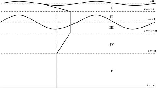
Figure 3. An example of the underlying current profile in the absence of waves, using the mean depth of the thermocline as the length scale. We distinguish four regions: (i) a subsurface layer $z\in [-1+l,0]$ in which a current of constant negative vorticity captures the salient features represented by a westward surface wind-induced drift, below which resides the EUC in the form of an eastward jet; (ii) the layer $z\in [-1-m,-1+l]$ in which the core of the EUC is represented by a uniform eastward current; (iii) the layer $z\in [-n,-1-m]$ in which a current of positive vorticity enables the transition to the practically motionless layer beneath it; (iv) the abyssal layer $z\in [-d,-n]$, not depicted in full, where we take the water to be stationary. The thermocline $z=-1$ is located in the second layer (the core of the EUC). Typical values are $l=m=1/3$, $n=2$ and $d=33$, corresponding to a thermocline depth of $120$ m, a subsurface layer of depth $80$ m where the effects of wind are noticeable, and an abyssal layer of practically motionless water beneath $240$ m, extending down to the ocean bed, located at a depth of $4$ km.

Our model for $U(z)$ contains six adjustable parameters, so not only can many variants of this flow profile be examined, but also we will be able to identify those factors that contribute most significantly to, for example, the speed of propagation of, and the strength of the coupling between, the surface and the internal waves. Further, it should be noted that this profile is constructed from regions of different, constant vorticities, the vorticity here being $U^{\prime }(z)$. So, reading from the surface downwards, we first have constant negative vorticity $-{\mathit{\gamma }}_{+}$ (with ${\mathit{\gamma }}_{+}=(V+W)/(1-l)$), then zero vorticity, which is followed by constant positive vorticity ${\mathit{\gamma }}_{-}=W/(n-1-m)$; finally, in the last region – the lowest region of the flow – we again have zero vorticity. Thus the vorticity distribution in the flow is prescribed by the undisturbed background state given in (36(36) $$\begin{array}{c}\hfill U(z)=\left\{\begin{array}{cccc}-V-z(V+W)/(1-l)\hfill & \hfill \text{for}& \hfill -1+l& <z\le 0,\hfill \\ W\hfill & \hfill \text{for}& \hfill -1-m& <z\le -1+l,\hfill \\ W(z+n)/(n-1-m)\hfill & \hfill \text{for}& \hfill -n& <z\le -1-m,\hfill \\ 0\hfill & \hfill \text{for}& \hfill -d& \le z\le -n,\hfill \end{array}\right.\end{array}$$(36) ) and, by virtue of our inviscid model for the flow, this vorticity remains unchanged for all time, as the flow and the waves interact and evolve. Thus any perturbations of this background flow that we introduce, e.g. wave disturbances superimposed on this background, must necessarily be irrotational. However, we should note that one consequence of the discontinuities in the vorticity is the appearance of corresponding discontinuities in the horizontal velocity component (although, of course, no such difficulties arise with the vertical component or the pressure, which are both continuous throughout the flow field).

This background flow must be maintained by a background pressure-distribution, $P(z)$, which is defined by the equations$$-2\mathit{\Omega }U(z)=-P^{\prime }(z)-1\text{for}-1<z<0\text{and}P=P_0\text{on}z=0,$$

for the region above the thermocline (by virtue of (20) and (23(23) $$\begin{array}{cccc}\hfill P(z)+p=& P_0\text{on}\hfill & \hfill z=& \mathit{\epsilon }\mathit{\eta }(x,t),\hfill \end{array}$$(23) )), and$$-2\mathit{\Omega }U(z)=-\frac{1}{1+r}{P}^{\prime }(z)-1\text{for}-d<z<-1,$$

below the thermocline, from (21); $P(z)$ is to be continuous across the thermocline (at $z=-1$), by (26(26) $$\begin{array}{cccc}\hfill P(z)+p(x,z,t)& \text{is continuous across}\hfill & \hfill z=& -1+\mathit{\epsilon }H(x,t),\hfill \end{array}$$(26) ). The pressure distribution is readily obtained; we find that(37) $$\begin{array}{c}\hfill P(z)=\left\{\begin{array}{cccc}{P}_0-z-\mathit{\Omega }z[2V+z(V+W)/(1-l)]\hfill & \hfill \text{for}& \hfill -1+l& \le z\le 0,\hfill \\ A+(2\mathit{\Omega }W-1)z\hfill & \hfill \text{for}& \hfill -1& \le z\le -1+l,\hfill \\ B+(1+r)(2\mathit{\Omega }W-1)z\hfill & \hfill \text{for}& \hfill -1-m& \le z\le -1,\hfill \\ C-(1+r)[z-\mathit{\Omega }W(2n+z)/(n-1-m)]\hfill & \hfill \text{for}& \hfill -n& \le z\le -1-m,\hfill \\ D-(1+r)z\hfill & \hfill \text{for}& \hfill -d& \le z\le -n,\hfill \end{array}\right.\end{array}$$(37)

where$$\begin{array}{cccc}\hfill A& =P_0+\mathit{\Omega }(V+W)(1-l),\hfill & \hfill B& =A+r(2\mathit{\Omega }W-1),\hfill \\ \hfill C& =B+\mathit{\Omega }W(1+r){(1+m)}^2/(n-1-m),\hfill & \hfill D& =C-n^2(1+r)\mathit{\Omega }W/(n-1-m).\hfill \end{array}$$

To put what we have just described in context, we quote some typical values of the six adjustable parameters, appropriate for the flow in the equatorial-Pacific-Ocean region:(38) $$\begin{array}{c}\hfill V\approx 0.015,W\approx 0.029,m=l\approx 0.33,n\approx 2,d\approx 33.\end{array}$$(38)

These correspond, via the non-dimensionalisation, (19(19) $$\begin{array}{cc}\hfill \overline{z}& =\overline{h}z,\overline{x}=\overline{h}x,\overline{t}=\overline{h}t/\sqrt{\overline{g}\overline{h}},\overline{\mathit{\eta }}=\overline{a}\mathit{\eta },\overline{H}=\overline{a}H,\hfill \\ \hfill (\overline{U}+\overline{u},\overline{w})& =\sqrt{\overline{g}\overline{h}}(U+u,w),\overline{P}+\overline{p}=\overline{{\mathit{\rho }}_0}\overline{g}\overline{h}(P+p),\hfill \end{array}$$(19) ), to a westward surface current of 0.5 ms${}^{-1}$ ($=\overline{V}$), and an eastward EUC peaking at 1 ms${}^{-1}$ ($=\overline{W}$), the EUC taken to be of width 40 m above and below the thermocline. The thermocline itself is at a depth of 120 m, the total depth of the ocean is 4 km, and below 240 m we have the abyssal region of stationary water; see the data provided by Johnson and McPhaden (2001). Indeed, we may use our model to fit the observations for other regions of the equatorial flow; for example, the choice of 120 m for the depth of the thermocline is actually appropriate for the 6000 km stretch between about 140${}^{\circ }$E and 150${}^{\circ }$W (see Fedorov and Brown 2009). Other slightly different choices can be made for other sections of the Equatorial Pacific. One other parameter appears in the expression (37(37) $$\begin{array}{c}\hfill P(z)=\left\{\begin{array}{cccc}{P}_0-z-\mathit{\Omega }z[2V+z(V+W)/(1-l)]\hfill & \hfill \text{for}& \hfill -1+l& \le z\le 0,\hfill \\ A+(2\mathit{\Omega }W-1)z\hfill & \hfill \text{for}& \hfill -1& \le z\le -1+l,\hfill \\ B+(1+r)(2\mathit{\Omega }W-1)z\hfill & \hfill \text{for}& \hfill -1-m& \le z\le -1,\hfill \\ C-(1+r)[z-\mathit{\Omega }W(2n+z)/(n-1-m)]\hfill & \hfill \text{for}& \hfill -n& \le z\le -1-m,\hfill \\ D-(1+r)z\hfill & \hfill \text{for}& \hfill -d& \le z\le -n,\hfill \end{array}\right.\end{array}$$(37) ) for $P(z)$, namely $\mathit{\Omega }$; this turns out to be rather smaller than any of the others quoted above: $\mathit{\Omega }\approx 2.5\times {10}^{-4}$. Its size would suggest that we should ignore this parameter at an early stage; however, even though it turns out to be rather unimportant in a numerical sense, we retain it because it embodies an intrinsic ingredient of the modelling.

Integration of (36(36) $$\begin{array}{c}\hfill U(z)=\left\{\begin{array}{cccc}-V-z(V+W)/(1-l)\hfill & \hfill \text{for}& \hfill -1+l& <z\le 0,\hfill \\ W\hfill & \hfill \text{for}& \hfill -1-m& <z\le -1+l,\hfill \\ W(z+n)/(n-1-m)\hfill & \hfill \text{for}& \hfill -n& <z\le -1-m,\hfill \\ 0\hfill & \hfill \text{for}& \hfill -d& \le z\le -n,\hfill \end{array}\right.\end{array}$$(36) ) over the entire depth yields ${\int }_{-d}^{0}U(z)\mathrm{d}z=\frac{1}{2}W(n+m+l)-\frac{1}{2}V(1-l).$ Multiplying this expression by $\overline{h}\sqrt{\overline{g}\overline{h}}$, by virtue of (19(19) $$\begin{array}{cc}\hfill \overline{z}& =\overline{h}z,\overline{x}=\overline{h}x,\overline{t}=\overline{h}t/\sqrt{\overline{g}\overline{h}},\overline{\mathit{\eta }}=\overline{a}\mathit{\eta },\overline{H}=\overline{a}H,\hfill \\ \hfill (\overline{U}+\overline{u},\overline{w})& =\sqrt{\overline{g}\overline{h}}(U+u,w),\overline{P}+\overline{p}=\overline{{\mathit{\rho }}_0}\overline{g}\overline{h}(P+p),\hfill \end{array}$$(19) ), we obtain the mass transport per unit width (in m${}^2$s${}^{-1}$). For a meridional width of 300 km, the values (38(38) $$\begin{array}{c}\hfill V\approx 0.015,W\approx 0.029,m=l\approx 0.33,n\approx 2,d\approx 33.\end{array}$$(38) ) predict a mass transport of about 40 Sv ($1\mathrm{Sv}={10}^6{\mathrm{m}}^3{\mathrm{s}}^{-1}$), thus corroborating the realistic nature of our model (see the field data in Izumo (2013)). Note that this feature highlights the difference between equatorial currents and the motion in a water tank: in a tank the vertical integral must vanish, but at the Equator the net eastward transport is compensated by a return flow at higher latitudes (see the discussion in Pacanowski and Philander (1980)).

We now return to our governing equations, (28)–(35(35) $$\begin{array}{cccc}\hfill w=& 0\text{on}\hfill & \hfill z=& -d.\hfill \end{array}$$(35) ), and incorporate our expressions for $U(z)$ and $P(z)$; it is immediately evident that, in each of the second equations in (28) and (29), an $\mathit{\epsilon }$ now cancels throughout. We may also note that the precise details of the pressure distribution appear only in their contributions to the boundary conditions at the surface and across the thermocline. On the other hand, the background velocity profile, $U(z)$, is very prominent in the Euler equation and will play a significant rôle in the construction of the solution. This is the stage at which we may present the full linear problem; with the equations in the form that we now have them, we allow $\mathit{\epsilon }\to 0$, keeping all the other parameters fixed, and retaining just the leading order, i.e. $\mathrm{O}(1)$. There is no evidence that waves of moderate amplitude (waves characterised by small $\mathit{\epsilon }$) have sufficient distance/time to allow nonlinearities to evolve to the extent that they become important (at least, over the length of the Pacific Equator – about 13000 km). Thus we may anticipate that the linear system will give an altogether reasonable description of the motion and its primary dynamics. However, we must expect that nonlinearity is likely to be important in other aspects of the wave dynamics. For example, if any critical layers appear – and they do – then the natural mechanism for describing their structure, within our inviscid system, is to invoke suitable nonlinearities; this idea is explored in appendix C. One of the overall aims in this study is to provide a sufficiently broad and robust framework in which further investigation is possible. The appearance of critical layers is an important area of current interest. These can trigger instabilities in marginally stable flows, and they are places where momentum and energy exchange between the waves and the mean flow can occur (see the discussion in Bühler (2009), Haynes (2003)); the evidence is accumulating as to their appearance and importance in EUC-type flows. (It is not appropriate, in this initial phase of the work, to give a lengthy and comprehensive description of the rôle of critical layers in these equatorial flows; however, our formulation and development should enable this to be a rich avenue for future studies.)

Thus our final model is a combination of a carefully-chosen background state, coupled with linearisation, but retaining all the other attributes of the model i.e. no other approximations are invoked; the problem described by equations (28)–(35(35) $$\begin{array}{cccc}\hfill w=& 0\text{on}\hfill & \hfill z=& -d.\hfill \end{array}$$(35) ) therefore becomes(39a) $$\begin{array}{cc}\hfill u_t+U(z)u_x+w{U}^{\prime }(z)+2\mathit{\Omega }w& =-p_x,\hfill \end{array}$$(39a) (39b) $$\begin{array}{cc}\hfill w_t+U(z)w_x-2\mathit{\Omega }u& =-p_z\hfill \end{array}$$(39b) in the region $(-1<z<0)$,(40a) $$\begin{array}{cc}\hfill u_t+U(z)u_x+w{U}^{\prime }(z)+2\mathit{\Omega }w& =-{\displaystyle \frac{p_x}{1+r}},\hfill \end{array}$$(40a) (40b) $$\begin{array}{cc}\hfill w_t+U(z)w_x-2\mathit{\Omega }u& =-{\displaystyle \frac{p_z}{1+r}}\hfill \end{array}$$(40b) in the region $(-d<z<-1)$, coupled with(41) $$\begin{array}{ccccc}\hfill u_x+w_z=& 0\hfill & \hfill \text{in}& -d<z\hfill & <0,\end{array}$$(41) (42) $$\begin{array}{ccccc}\hfill u_z-w_x=& 0\hfill & \hfill \text{in}& -d<z\hfill & <0,\end{array}$$(42) (43) $$\begin{array}{ccccc}\hfill p=& (1+2\mathit{\Omega }V)\mathit{\eta }\hfill & \hfill \text{on}& z\hfill & =0,\end{array}$$(43) (44) $$\begin{array}{ccccc}\hfill w=& {\mathit{\eta }}_t-V{\mathit{\eta }}_x\hfill & \hfill \text{on}& z\hfill & =0,\end{array}$$(44) (45) $$\begin{array}{ccccc}\hfill w=& H_t+W{H}_x\hfill & \hfill \text{on}& z\hfill & =-1,\end{array}$$(45) (46) $$\begin{array}{ccccc}\hfill p_a-p_b=& r(2\mathit{\Omega }W-1)H\hfill & \hfill \text{on}& z\hfill & =-1,\end{array}$$(46) (47) $$\begin{array}{ccccc}\hfill w=& 0\hfill & \hfill \text{on}& z\hfill & =-d,\end{array}$$(47)

with $U(z)$ given by (36(36) $$\begin{array}{c}\hfill U(z)=\left\{\begin{array}{cccc}-V-z(V+W)/(1-l)\hfill & \hfill \text{for}& \hfill -1+l& <z\le 0,\hfill \\ W\hfill & \hfill \text{for}& \hfill -1-m& <z\le -1+l,\hfill \\ W(z+n)/(n-1-m)\hfill & \hfill \text{for}& \hfill -n& <z\le -1-m,\hfill \\ 0\hfill & \hfill \text{for}& \hfill -d& \le z\le -n,\hfill \end{array}\right.\end{array}$$(36) ); the subscripts $a$, $b$, in $p_a$ and $p_b$, refer to the limits of $p$ from “above” and “below” $z=-1$. The most obvious simplification evident here, due to the linearisation, is that evaluation on unknown lines – the general positions of the free surface and the thermocline – has been replaced by evaluation on known lines, namely $z=0$ and $z=-1$, respectively. We have therefore, equivalently, mapped the problem from one with unknown boundaries to one with known boundaries, a procedure that can be rigorously justified. (Here, because of the nature of this problem, this is nothing more than recognising that the relevant Taylor expansions are valid approximations to the weakly nonlinear problem: the higher-order terms in $\mathit{\epsilon }$ merely contribute uniformly small corrections to the linear solution.) We note that this system, (39)–(47(47) $$\begin{array}{ccccc}\hfill w=& 0\hfill & \hfill \text{on}& z\hfill & =-d,\end{array}$$(47) ), retains all the other parameters $(\mathit{\Omega },r,d)$, held fixed as the limiting process to linearisation is performed, as well as incorporating all the details of the background flow, $U(z)$.

One consequence of the linearisation is that, from the pressure distribution (37(37) $$\begin{array}{c}\hfill P(z)=\left\{\begin{array}{cccc}{P}_0-z-\mathit{\Omega }z[2V+z(V+W)/(1-l)]\hfill & \hfill \text{for}& \hfill -1+l& \le z\le 0,\hfill \\ A+(2\mathit{\Omega }W-1)z\hfill & \hfill \text{for}& \hfill -1& \le z\le -1+l,\hfill \\ B+(1+r)(2\mathit{\Omega }W-1)z\hfill & \hfill \text{for}& \hfill -1-m& \le z\le -1,\hfill \\ C-(1+r)[z-\mathit{\Omega }W(2n+z)/(n-1-m)]\hfill & \hfill \text{for}& \hfill -n& \le z\le -1-m,\hfill \\ D-(1+r)z\hfill & \hfill \text{for}& \hfill -d& \le z\le -n,\hfill \end{array}\right.\end{array}$$(37) ), the pressure condition (34(34) $$\begin{array}{cccc}\hfill P(z)+\mathit{\epsilon }p(x,z,t& )\text{is continuous across}\hfill & \hfill z=& -1+\mathit{\epsilon }H(x,t),\hfill \end{array}$$(34) ) becomes $P_0-\mathit{\epsilon }\mathit{\eta }-\mathit{\Omega }[2V+\mathit{\epsilon }\mathit{\eta }(V+W)/(1-l)]\mathit{\epsilon }\mathit{\eta }+\mathit{\epsilon }p=P_0$ on $z=\mathit{\epsilon }\mathit{\eta }$, which, to leading order in $\mathit{\epsilon }$, gives $p=(1+2\mathit{\Omega }V)\mathit{\eta }$ on $z=0$, as quoted in (43(43) $$\begin{array}{ccccc}\hfill p=& (1+2\mathit{\Omega }V)\mathit{\eta }\hfill & \hfill \text{on}& z\hfill & =0,\end{array}$$(43) ) above. Further, the condition that $P+\mathit{\epsilon }p$ must be continuous across the thermocline (see (34(34) $$\begin{array}{cccc}\hfill P(z)+\mathit{\epsilon }p(x,z,t& )\text{is continuous across}\hfill & \hfill z=& -1+\mathit{\epsilon }H(x,t),\hfill \end{array}$$(34) )), with $P$, given by (37(37) $$\begin{array}{c}\hfill P(z)=\left\{\begin{array}{cccc}{P}_0-z-\mathit{\Omega }z[2V+z(V+W)/(1-l)]\hfill & \hfill \text{for}& \hfill -1+l& \le z\le 0,\hfill \\ A+(2\mathit{\Omega }W-1)z\hfill & \hfill \text{for}& \hfill -1& \le z\le -1+l,\hfill \\ B+(1+r)(2\mathit{\Omega }W-1)z\hfill & \hfill \text{for}& \hfill -1-m& \le z\le -1,\hfill \\ C-(1+r)[z-\mathit{\Omega }W(2n+z)/(n-1-m)]\hfill & \hfill \text{for}& \hfill -n& \le z\le -1-m,\hfill \\ D-(1+r)z\hfill & \hfill \text{for}& \hfill -d& \le z\le -n,\hfill \end{array}\right.\end{array}$$(37) ), expressed in terms of the Heaviside step function $\mathcal{H}$ by$$\begin{array}{cc}\hfill P(z)=A+1-2\mathit{\Omega }W+(1+r)(2\mathit{\Omega }W-1)(z+1)-r(2\mathit{\Omega }W-1)& (z+1)\mathcal{H}(z+1)\hfill \\ \hfill & \text{near}z=-1,\hfill \end{array}$$

recovers (46(46) $$\begin{array}{ccccc}\hfill p_a-p_b=& r(2\mathit{\Omega }W-1)H\hfill & \hfill \text{on}& z\hfill & =-1,\end{array}$$(46) ) when evaluated at order $\mathit{\epsilon }$ on $z=-1+\mathit{\epsilon }H$. Equation (42(42) $$\begin{array}{ccccc}\hfill u_z-w_x=& 0\hfill & \hfill \text{in}& -d<z\hfill & <0,\end{array}$$(42) ) is the requirement that any perturbation of the underlying background state must be irrotational (as we discussed earlier).

Figure 4. Sketch of the five fluid regions that are relevant to the solution of the linear problem.

We make one final, general observation before we present our analysis of equations (39)–(47(47) $$\begin{array}{ccccc}\hfill w=& 0\hfill & \hfill \text{on}& z\hfill & =-d,\end{array}$$(47) ). The development of these equations is based on the single limiting process $\mathit{\epsilon }\to 0$, keeping all the other parameters fixed. Thus none are ignored at this stage – we commented on the size of $\mathit{\Omega }$ above – but to do so is equivalent to regarding them as functions of $\mathit{\epsilon }$, which patently they are not (on physical grounds). It is in this sense that we have developed the most general linear problem of this phenomenon, restricted – but not by much – only by the choice of the background state. Of course, as we have already mentioned, some of the remaining parameters are numerically small, and this can be to our advantage later: we can use this property to obtain some simple, but useful estimates.

3. Solution of the linear problem

The development of the solution of the system (39)–(47(47) $$\begin{array}{ccccc}\hfill w=& 0\hfill & \hfill \text{on}& z\hfill & =-d,\end{array}$$(47) ) involves the examination of five regions: $0>z>-1+l$, $-1+l>z>-1$, $-1>z>-1-m$, $-1-m>z>-n$, $-n>z>-d$; we refer to these as Regions I-V, respectively, which are shown in figure 4. The most convenient approach for solving this problem is to start from the bottom (Region V) and work upwards. We seek a single, general harmonic mode with wave number $k$ (which we take to be positive throughout); then, because the system is linear, we may later add together any number of such modes. One possibility is to add an infinity of modes or, equivalently, to integrate over the wave number in order to construct a more general solution (and this would allow the inclusion of some suitable initial data). However, we aim for a simpler approach: we assume that suitable initial data exist that give rise to the solution that we seek here. It is sufficient, for our purposes, to limit our choice to just two modes: typically, a short-wavelength gravity wave (at the surface) combined with a very-long-wavelength component of (probably) very small amplitude. It is this long-wave contribution to the surface wave, as we shall see, which will provide the driver for the wave on the thermocline. We will now present the main results obtained by solving in each region; we will also quote the specific version of the equations and boundary conditions as they relate to that region, to aid the reader.

3.1. Region V

The equations valid in this region are$$\begin{array}{cc}\hfill \left.\begin{array}{c}\hfill u_t+2\mathit{\Omega }w=-{\displaystyle \frac{p_x}{1+r}}\\ \hfill w_t-2\mathit{\Omega }u=-{\displaystyle \frac{p_z}{1+r}}\\ \hfill u_x+w_z=0\text{and}{u}_z-w_x=0\end{array}\right\}& \text{in}-d<z<-n,\hfill \\ \hfill [0.6em]w=0& \text{on}z=-d,\hfill \end{array}$$

with the following single-harmonic-mode solution$$\begin{array}{cc}& w=E({\mathrm{e}}^{kz}-{\mathrm{e}}^{-2kd-kz})sin(k\mathit{\xi }),u=E({\mathrm{e}}^{kz}+{\mathrm{e}}^{-2kd-kz})cos(k\mathit{\xi }),\hfill \\ \hfill & p=E(1+r)[c({\mathrm{e}}^{kz}+{\mathrm{e}}^{-2kd-kz})+{\displaystyle \frac{2\mathit{\Omega }}{k}}({\mathrm{e}}^{kz}-{\mathrm{e}}^{-2kd-kz})]cos(k\mathit{\xi }),\hfill \end{array}$$

where $\mathit{\xi }=x-c(k)t$, so that $c$ is the speed of the wave; $E$ is an arbitrary (real) constant.

3.2. Region IV

The equations in the region $(-n<z<-1-m)$ are$$\begin{array}{cc}\hfill u_t+{\mathit{\gamma }}_{-}(z+n)u_x+{\mathit{\gamma }}_{-}w+2\mathit{\Omega }w& =-{\displaystyle \frac{p_x}{1+r}},\hfill \\ \hfill w_t+{\mathit{\gamma }}_{-}(z+n)w_x-2\mathit{\Omega }u& =-{\displaystyle \frac{p_z}{1+r}},\hfill \end{array}$$$$\begin{array}{cc}& u_x+w_z=0\text{and}{u}_z-w_x=0,\hfill \end{array}$$

where ${\mathit{\gamma }}_{-}=W/(n-1-m)$. The general solution that corresponds to the solution in Region V, is$$\begin{array}{cc}& w=(F{\mathrm{e}}^{kz}+G{\mathrm{e}}^{-kz})sin(k\mathit{\xi }),u=(F{\mathrm{e}}^{kz}-G{\mathrm{e}}^{-kz})cos(k\mathit{\xi }),\hfill \\ \hfill & p=(1+r)[[c-{\mathit{\gamma }}_{-}(z+n)](F{\mathrm{e}}^{kz}-G{\mathrm{e}}^{-kz})+{\displaystyle \frac{2\mathit{\Omega }+{\mathit{\gamma }}_{-}}{k}}(F{\mathrm{e}}^{kz}+G{\mathrm{e}}^{-kz})]cos(k\mathit{\xi }),\hfill \end{array}$$

where $F$ and $G$ are some constants. The solution that we seek must, of course, satisfy suitable continuity conditions at the boundaries between the regions. Indeed, this requirement, coupled with the number of regions, is the main complicating factor in the calculation, even though the individual solutions are readily constructed. The fundamental physical requirement of the continuity of $w$ and of $p$ at the V/IV boundary ($z=-n$) gives, respectively,(48) $$\begin{array}{c}\hfill F{e}_n+G=E(e_n-e_d)\end{array}$$(48)

and(49) $$\begin{array}{c}\hfill c(F{e}_n-G)+{\displaystyle \frac{2\mathit{\Omega }+{\mathit{\gamma }}_{-}}{k}}(F{e}_n+G)=E[c(e_n+e_d)+{\displaystyle \frac{2\mathit{\Omega }}{k}}(e_n-e_d)],\end{array}$$(49)

where $e_n={\mathrm{e}}^{-2kn}$ and $e_d={\mathrm{e}}^{-2kd}$. (The calculation will involve a number of exponential terms, containing various exponents; we adopt a simple shorthand to identify each of these, and each has the property that it tends to zero as $k\to \infty$.) Imposing the additional continuity of $u$ at the IV/V boundary would yield the further condition$$F{e}_n-G=E(e_n+e_d).$$

It is easy to see that this and (48(48) $$\begin{array}{c}\hfill F{e}_n+G=E(e_n-e_d)\end{array}$$(48) ) force $F=E$ and $G=-E{e}_d$, which are incompatible with (49(49) $$\begin{array}{c}\hfill c(F{e}_n-G)+{\displaystyle \frac{2\mathit{\Omega }+{\mathit{\gamma }}_{-}}{k}}(F{e}_n+G)=E[c(e_n+e_d)+{\displaystyle \frac{2\mathit{\Omega }}{k}}(e_n-e_d)],\end{array}$$(49) ). These considerations show that discontinuities in $u$ are inherent within our inviscid model: they are a consequence of an irrotational perturbation that is driven by a background flow which exhibits jumps in vorticity.

From (48(48) $$\begin{array}{c}\hfill F{e}_n+G=E(e_n-e_d)\end{array}$$(48) ) and (49(49) $$\begin{array}{c}\hfill c(F{e}_n-G)+{\displaystyle \frac{2\mathit{\Omega }+{\mathit{\gamma }}_{-}}{k}}(F{e}_n+G)=E[c(e_n+e_d)+{\displaystyle \frac{2\mathit{\Omega }}{k}}(e_n-e_d)],\end{array}$$(49) ), elimination of $E$ produces(50) $$\begin{array}{c}\hfill G={\displaystyle \frac{{\mathit{\gamma }}_{-}(1-e_{dn})-2ck{e}_{dn}}{2ck-{\mathit{\gamma }}_{-}(1-e_{dn})}}F{e}_n,\end{array}$$(50)

where $e_{dn}={\mathrm{e}}^{-2(d-n)k}$.

3.3. Region III

This region, $(-1-m<z<-1)$, is directly below the thermocline; the equations here are$$\begin{array}{cc}& u_t+W{u}_x+2\mathit{\Omega }w=-{\displaystyle \frac{p_x}{1+r}},\hfill \\ \hfill & w_t+W{w}_x-2\mathit{\Omega }u=-{\displaystyle \frac{p_z}{1+r}},\hfill \\ \hfill & u_x+w_z=0\text{and}{u}_z-w_x=0,\hfill \end{array}$$

with the solution$$\begin{array}{cc}& w=(M{\mathrm{e}}^{kz}+N{\mathrm{e}}^{-kz})sin(k\mathit{\xi }),u=(M{\mathrm{e}}^{kz}-N{\mathrm{e}}^{-kz})cos(k\mathit{\xi }),\hfill \\ \hfill & p=(1+r)[(c-W)(M{\mathrm{e}}^{kz}-N{\mathrm{e}}^{-kz})+{\displaystyle \frac{2\mathit{\Omega }}{k}}(M{\mathrm{e}}^{kz}+N{\mathrm{e}}^{-kz})]cos(k\mathit{\xi }),\hfill \end{array}$$

where $M$ and $N$ are constants appropriate to this region. In terms of $e_m={\mathrm{e}}^{-2(1+m)k}$, we can write the requirement that $w$ and $p$ are continuous at $z=-1-m$ as, respectively, the conditions$$M{e}_m+N=F{e}_m+G$$

and$$(c-W)(M{e}_m-N)+{\displaystyle \frac{2\mathit{\Omega }}{k}}(M{e}_m+N)=(c-W)(F{e}_m-G)+{\displaystyle \frac{2\mathit{\Omega }+{\mathit{\gamma }}_{-}}{k}}(F{e}_m+G).$$

From this pair, combined with (50(50) $$\begin{array}{c}\hfill G={\displaystyle \frac{{\mathit{\gamma }}_{-}(1-e_{dn})-2ck{e}_{dn}}{2ck-{\mathit{\gamma }}_{-}(1-e_{dn})}}F{e}_n,\end{array}$$(50) ), we can obtain expressions for $M$ and $N$ (essentially in terms of $F$):(51) $$\begin{array}{cc}\hfill 2k(c-W)\left(2c-{\displaystyle \frac{{\mathit{\gamma }}_{-}(1-e_{dn})}{k}}\right){\displaystyle \frac{M{e}_m}{F}}& ={\displaystyle \frac{{\mathit{\gamma }}_{-}^2(1-e_{dn})(e_n-e_m)}{k}}+4ck(c-W)e_m\hfill \\ \hfill & +2{\mathit{\gamma }}_{-}\left(c(e_{dnm}-e_d)+W(e_m-e_{dnm})\right),\hfill \end{array}$$(51)

where $e_{dnm}={\mathrm{e}}^{-2(d-n+1+m)k}$, and(52) $$\begin{array}{cc}\hfill 2k(c-W)\left(2c-{\displaystyle \frac{{\mathit{\gamma }}_{-}(1-e_{dn})}{k}}\right){\displaystyle \frac{N}{F}}=& {\displaystyle \frac{{\mathit{\gamma }}_{-}^2(1-e_{dn})(e_m-e_n)}{k}}-4ck(c-W)e_d\hfill \\ \hfill & +2{\mathit{\gamma }}_{-}(c(e_n-e_m)-W(e_n-e_d)).\hfill \end{array}$$(52)

3.4. Region II

This is the region $(-1<z<-1+l)$, directly above the thermocline (across which, in our model, the speed of the EUC is constant); the governing equations are$$\begin{array}{cc}& u_t+W{u}_x+2\mathit{\Omega }w=-p_x,\hfill \\ \hfill & w_t+W{w}_x-2\mathit{\Omega }u=-p_z,\hfill \\ \hfill & u_x+w_z=0\text{and}{u}_z-w_x=0.\hfill \end{array}$$

The solution here is$$\begin{array}{cc}& w=(S{\mathrm{e}}^{kz}+R{\mathrm{e}}^{-kz})sin(k\mathit{\xi }),u=(S{\mathrm{e}}^{kz}-R{\mathrm{e}}^{-kz})cos(k\mathit{\xi }),\hfill \\ \hfill & p=[(c-W)(S{\mathrm{e}}^{kz}-R{\mathrm{e}}^{-kz})+{\displaystyle \frac{2\mathit{\Omega }}{k}}(S{\mathrm{e}}^{kz}+R{\mathrm{e}}^{-kz})]cos(k\mathit{\xi }),\hfill \end{array}$$

where $S$ and $R$ are suitable constants. We now need to apply the important conditions that pertain across the thermocline; first we have the kinematic condition (45(45) $$\begin{array}{ccccc}\hfill w=& H_t+W{H}_x\hfill & \hfill \text{on}& z\hfill & =-1,\end{array}$$(45) ), which requires(53) $$\begin{array}{c}\hfill (M{\mathrm{e}}^{-k}+N{\mathrm{e}}^k)sin(k\mathit{\xi })=(S{\mathrm{e}}^{-k}+R{\mathrm{e}}^k)sin(k\mathit{\xi })=H_t+W{H}_x.\end{array}$$(53)

The pressure condition across the thermocline, (46(46) $$\begin{array}{ccccc}\hfill p_a-p_b=& r(2\mathit{\Omega }W-1)H\hfill & \hfill \text{on}& z\hfill & =-1,\end{array}$$(46) ), results in(54) $$\begin{array}{cc}& \{(c-W)(S{\mathrm{e}}^{-k}-R{\mathrm{e}}^k)+{\displaystyle \frac{2\mathit{\Omega }}{k}}(S{\mathrm{e}}^{-k}+R{\mathrm{e}}^k)\hfill \\ \hfill & -(1+r)[(c-W)(M{\mathrm{e}}^{-k}-N{\mathrm{e}}^k)+{\displaystyle \frac{2\mathit{\Omega }}{k}}(M{\mathrm{e}}^{-k}+N{\mathrm{e}}^k)]\}cos(k\mathit{\xi })\hfill \\ \hfill & =r(2\mathit{\Omega }W-1)H.\hfill \end{array}$$(54)

The first of this pair, (53(53) $$\begin{array}{c}\hfill (M{\mathrm{e}}^{-k}+N{\mathrm{e}}^k)sin(k\mathit{\xi })=(S{\mathrm{e}}^{-k}+R{\mathrm{e}}^k)sin(k\mathit{\xi })=H_t+W{H}_x.\end{array}$$(53) ), yields$$M{e}_2+N=S{e}_2+R,$$

where $e_2={\mathrm{e}}^{-2k}$, and the second, (54(54) $$\begin{array}{cc}& \{(c-W)(S{\mathrm{e}}^{-k}-R{\mathrm{e}}^k)+{\displaystyle \frac{2\mathit{\Omega }}{k}}(S{\mathrm{e}}^{-k}+R{\mathrm{e}}^k)\hfill \\ \hfill & -(1+r)[(c-W)(M{\mathrm{e}}^{-k}-N{\mathrm{e}}^k)+{\displaystyle \frac{2\mathit{\Omega }}{k}}(M{\mathrm{e}}^{-k}+N{\mathrm{e}}^k)]\}cos(k\mathit{\xi })\hfill \\ \hfill & =r(2\mathit{\Omega }W-1)H.\hfill \end{array}$$(54) ), is to be consistent with the first, when $H$ is eliminated; this can be written as(55) $$\begin{array}{cc}& (c-W)(S{e}_2-R)+{\displaystyle \frac{2\mathit{\Omega }}{k}}(S{e}_2+R)\hfill \\ \hfill & -(1+r)[(c-W)(M{e}_2-N)+{\displaystyle \frac{2\mathit{\Omega }}{k}}(M{e}_2+N)]={\displaystyle \frac{r(2\mathit{\Omega }W-1)}{k(c-W)}}(M{e}_2+N).\hfill \end{array}$$(55)

The previous two displayed relations enable us to determine $S$ and $R$ in terms of $M$ and $N$:(56) $$\begin{array}{c}\hfill S=M+{\displaystyle \frac{r}{2}}[M-{\displaystyle \frac{N}{e_2}}+{\displaystyle \frac{2\mathit{\Omega }c-1}{k{(c-W)}^2}}(M+{\displaystyle \frac{N}{e_2}})]\end{array}$$(56)

and(57) $$\begin{array}{c}\hfill R=N-{\displaystyle \frac{r{e}_2}{2}}[M-{\displaystyle \frac{N}{e_2}}+{\displaystyle \frac{2\mathit{\Omega }c-1}{k{(c-W)}^2}}(M+{\displaystyle \frac{N}{e_2}})].\end{array}$$(57)

3.5. Region I

The governing equations in the uppermost region $(-1+l<z<0)$ are$$\begin{array}{cc}\hfill u_t-(V+{\mathit{\gamma }}_{+}z)u_x-{\mathit{\gamma }}_{+}w+2\mathit{\Omega }w& =-p_x,\hfill \\ \hfill w_t-(V+{\mathit{\gamma }}_{+}z)w_x-2\mathit{\Omega }u& =-p_z,\hfill \\ \hfill u_x+w_z=0\text{and}{u}_z-w_x& =0,\hfill \end{array}$$

coupled with the boundary conditions$$\begin{array}{cc}\hfill p& =(1+2\mathit{\Omega }V)\mathit{\eta }\text{on}z=0,\hfill \\ \hfill w& ={\mathit{\eta }}_t-V{\mathit{\eta }}_x\text{on}z=0,\hfill \end{array}$$

where ${\mathit{\gamma }}_{+}=(V+W)/(1-l)$. The solution here is of the form$$\begin{array}{cc}& w=(A{\mathrm{e}}^{kz}+B{\mathrm{e}}^{-kz})sin(k\mathit{\xi }),u=(A{\mathrm{e}}^{kz}-B{\mathrm{e}}^{-kz})cos(k\mathit{\xi }),\hfill \\ \hfill & p=[(c+V+{\mathit{\gamma }}_{+}z)(A{\mathrm{e}}^{kz}-B{\mathrm{e}}^{-kz})+{\displaystyle \frac{2\mathit{\Omega }-{\mathit{\gamma }}_{+}}{k}}(A{\mathrm{e}}^{kz}+B{\mathrm{e}}^{-kz})]cos(k\mathit{\xi }),\hfill \end{array}$$

where $A$ and $B$ are constants to be determined. The two conditions at $z=0$ require$$(1+2\mathit{\Omega }V)\mathit{\eta }=[(c+V)(A-B)+{\displaystyle \frac{2\mathit{\Omega }-{\mathit{\gamma }}_{+}}{k}}(A+B)]cos(k\mathit{\xi })$$

and(58) $$\begin{array}{c}\hfill {\mathit{\eta }}_t-V{\mathit{\eta }}_x=(A+B)sin(k\mathit{\xi }),\end{array}$$(58)

respectively; these two are consistent (when $\mathit{\eta }$ is eliminated) if(59) $$\begin{array}{c}\hfill ({\displaystyle \frac{1+2\mathit{\Omega }V}{c+V}}-2\mathit{\Omega }+{\mathit{\gamma }}_{+})({\displaystyle \frac{A+B}{A-B}})=k(c+V),\end{array}$$(59)

which provides the fundamental dispersion relation for this system. The apparent simplicity of this expression hides the very considerable complexity of the coefficient $(A+B)/(A-B)$, as is evident from all the preceding expressions for the various constants, together with the final set of relations that are needed to complete the specification of the solution. The continuity of $w$ and of $p$ at the II/I boundary ($z=-1+l$) give, respectively,$$A{e}_l+B=S{e}_l+R$$

and$$(c-W)(S{e}_l-R)+{\displaystyle \frac{2\mathit{\Omega }}{k}}(S{e}_l+R)=(c-W)(A{e}_l-B)+{\displaystyle \frac{2\mathit{\Omega }-{\mathit{\gamma }}_{+}}{k}}(A{e}_l+B),$$

where $e_l={\mathrm{e}}^{-2(1-l)k}$. These equations provide us with expressions for $A$ and $B$:$$A=S+{\displaystyle \frac{{\mathit{\gamma }}_{+}}{2k(c-W)}}(S+{\displaystyle \frac{R}{e_l}}),B=R-{\displaystyle \frac{{\mathit{\gamma }}_{+}}{2k(c-W)}}(S{e}_l+R),$$

which in turn lead to expressions for $A+B$ and $A-B$, if we take (56(56) $$\begin{array}{c}\hfill S=M+{\displaystyle \frac{r}{2}}[M-{\displaystyle \frac{N}{e_2}}+{\displaystyle \frac{2\mathit{\Omega }c-1}{k{(c-W)}^2}}(M+{\displaystyle \frac{N}{e_2}})]\end{array}$$(56) )–(57(57) $$\begin{array}{c}\hfill R=N-{\displaystyle \frac{r{e}_2}{2}}[M-{\displaystyle \frac{N}{e_2}}+{\displaystyle \frac{2\mathit{\Omega }c-1}{k{(c-W)}^2}}(M+{\displaystyle \frac{N}{e_2}})].\end{array}$$(57) ) into account:(60) $$\begin{array}{cc}\hfill A+B& =(1+\mathit{\theta }-\mathit{\theta }{e}_l)M+(1-\mathit{\theta }+{\displaystyle \frac{\mathit{\theta }}{e_l}})N+{\displaystyle \frac{r\mathit{\lambda }}{2}}[1-e_2+\mathit{\theta }(1+e_2-e_{2l}-e_l)];\hfill \end{array}$$(60) (61) $$\begin{array}{cc}\hfill A-B& =(1+\mathit{\theta }+\mathit{\theta }{e}_l)M-(1-\mathit{\theta }-{\displaystyle \frac{\mathit{\theta }}{e_l}})N+{\displaystyle \frac{r\mathit{\lambda }}{2}}[1+e_2+\mathit{\theta }(1+e_l-e_{2l}-e_2)];\hfill \end{array}$$(61)

where$$\begin{array}{c}\hfill \mathit{\lambda }=M-{\displaystyle \frac{N}{e_2}}+{\displaystyle \frac{2\mathit{\Omega }c-1}{k{(c-W)}^2}}(M+{\displaystyle \frac{N}{e_2}}),\end{array}$$(62) $$\begin{array}{c}\hfill \mathit{\theta }={\displaystyle \frac{{\mathit{\gamma }}_{+}}{2k(c-W)}},e_{2l}={\mathrm{e}}^{-2lk}={\displaystyle \frac{e_2}{e_l}}.\end{array}$$(62)

From (51(51) $$\begin{array}{cc}\hfill 2k(c-W)\left(2c-{\displaystyle \frac{{\mathit{\gamma }}_{-}(1-e_{dn})}{k}}\right){\displaystyle \frac{M{e}_m}{F}}& ={\displaystyle \frac{{\mathit{\gamma }}_{-}^2(1-e_{dn})(e_n-e_m)}{k}}+4ck(c-W)e_m\hfill \\ \hfill & +2{\mathit{\gamma }}_{-}\left(c(e_{dnm}-e_d)+W(e_m-e_{dnm})\right),\hfill \end{array}$$(51) ) and (52(52) $$\begin{array}{cc}\hfill 2k(c-W)\left(2c-{\displaystyle \frac{{\mathit{\gamma }}_{-}(1-e_{dn})}{k}}\right){\displaystyle \frac{N}{F}}=& {\displaystyle \frac{{\mathit{\gamma }}_{-}^2(1-e_{dn})(e_m-e_n)}{k}}-4ck(c-W)e_d\hfill \\ \hfill & +2{\mathit{\gamma }}_{-}(c(e_n-e_m)-W(e_n-e_d)).\hfill \end{array}$$(52) ), coupled with (60(60) $$\begin{array}{cc}\hfill A+B& =(1+\mathit{\theta }-\mathit{\theta }{e}_l)M+(1-\mathit{\theta }+{\displaystyle \frac{\mathit{\theta }}{e_l}})N+{\displaystyle \frac{r\mathit{\lambda }}{2}}[1-e_2+\mathit{\theta }(1+e_2-e_{2l}-e_l)];\hfill \end{array}$$(60) )–(61(61) $$\begin{array}{cc}\hfill A-B& =(1+\mathit{\theta }+\mathit{\theta }{e}_l)M-(1-\mathit{\theta }-{\displaystyle \frac{\mathit{\theta }}{e_l}})N+{\displaystyle \frac{r\mathit{\lambda }}{2}}[1+e_2+\mathit{\theta }(1+e_l-e_{2l}-e_2)];\hfill \end{array}$$(61) ), the complicated nature of the dispersion relation is now quite evident. Nevertheless, it turns out to be possible to develop some fairly simple special cases (based essentially on short- or long-wave limits). Of course, it is always open to us to examine the dispersion relation in a purely numerical fashion, perhaps choosing values for all the parameters, and then attempting to seek solutions for $c$ as a function of $k$. Even this is a daunting exercise because equation (59(59) $$\begin{array}{c}\hfill ({\displaystyle \frac{1+2\mathit{\Omega }V}{c+V}}-2\mathit{\Omega }+{\mathit{\gamma }}_{+})({\displaystyle \frac{A+B}{A-B}})=k(c+V),\end{array}$$(59) ) is not some simple polynomial in $c$. We shall demonstrate what is possible and accessible when we discuss various special limiting cases; see sections 4 and 5. Nevertheless, it is clear that the development presented here, for the chosen background velocity profile, constitutes an exact solution of the two-dimensional linear problem in the $f$-plane approximation.

One other important element in any examination of this problem is the relation that exists between the amplitudes of the waves at the surface and on the thermocline. Let us take the surface wave to be $\mathit{\eta }=acos(k\mathit{\xi })$, which is consistent with the harmonic structure that we have introduced; then from equation (58(58) $$\begin{array}{c}\hfill {\mathit{\eta }}_t-V{\mathit{\eta }}_x=(A+B)sin(k\mathit{\xi }),\end{array}$$(58) ) we obtain(63) $$\begin{array}{c}\hfill A+B=ak(c+V).\end{array}$$(63)

Correspondingly, if the oscillation of the thermocline is given as $H=\mathit{\Delta }cos(k\mathit{\xi })$, then from equation (53(53) $$\begin{array}{c}\hfill (M{\mathrm{e}}^{-k}+N{\mathrm{e}}^k)sin(k\mathit{\xi })=(S{\mathrm{e}}^{-k}+R{\mathrm{e}}^k)sin(k\mathit{\xi })=H_t+W{H}_x.\end{array}$$(53) ), we have(64) $$\begin{array}{c}\hfill M{\mathrm{e}}^{-k}+N{\mathrm{e}}^k=\mathit{\Delta }k(c-W).\end{array}$$(64)

We shall demonstrate that it is possible, given either $a$ or $\mathit{\Delta }$, to determine the other from our analysis presented above. The results that we obtain will then clarify the strength and structure of the coupling between the surface wave and the internal wave at the thermocline.

4. Short waves

The simplest case is that of short waves, i.e. $k\to \infty$. We note from (51(51) $$\begin{array}{cc}\hfill 2k(c-W)\left(2c-{\displaystyle \frac{{\mathit{\gamma }}_{-}(1-e_{dn})}{k}}\right){\displaystyle \frac{M{e}_m}{F}}& ={\displaystyle \frac{{\mathit{\gamma }}_{-}^2(1-e_{dn})(e_n-e_m)}{k}}+4ck(c-W)e_m\hfill \\ \hfill & +2{\mathit{\gamma }}_{-}\left(c(e_{dnm}-e_d)+W(e_m-e_{dnm})\right),\hfill \end{array}$$(51) ) and (62(62) $$\begin{array}{c}\hfill \mathit{\theta }={\displaystyle \frac{{\mathit{\gamma }}_{+}}{2k(c-W)}},e_{2l}={\mathrm{e}}^{-2lk}={\displaystyle \frac{e_2}{e_l}}.\end{array}$$(62) ) that both $M$ and $\mathit{\lambda }$ contain terms that grow exponentially. (Our notation for the exponential terms, $e_q$, has been adopted so that all these contain negative exponents, i.e. they all decay for large $k$.) Note that$$\mathit{\lambda }=M{m}_{+}+{\displaystyle \frac{N}{e_2}}{m}_{-}\text{with}{m}_{\pm }={\displaystyle \frac{2\mathit{\Omega }c-1}{k{(c-W)}^2}}\pm 1,$$

while (51(51) $$\begin{array}{cc}\hfill 2k(c-W)\left(2c-{\displaystyle \frac{{\mathit{\gamma }}_{-}(1-e_{dn})}{k}}\right){\displaystyle \frac{M{e}_m}{F}}& ={\displaystyle \frac{{\mathit{\gamma }}_{-}^2(1-e_{dn})(e_n-e_m)}{k}}+4ck(c-W)e_m\hfill \\ \hfill & +2{\mathit{\gamma }}_{-}\left(c(e_{dnm}-e_d)+W(e_m-e_{dnm})\right),\hfill \end{array}$$(51) )–(52(52) $$\begin{array}{cc}\hfill 2k(c-W)\left(2c-{\displaystyle \frac{{\mathit{\gamma }}_{-}(1-e_{dn})}{k}}\right){\displaystyle \frac{N}{F}}=& {\displaystyle \frac{{\mathit{\gamma }}_{-}^2(1-e_{dn})(e_m-e_n)}{k}}-4ck(c-W)e_d\hfill \\ \hfill & +2{\mathit{\gamma }}_{-}(c(e_n-e_m)-W(e_n-e_d)).\hfill \end{array}$$(52) ) yield $M\sim F$ and $N\sim -F{e}_d$ as $k\to \infty$. Thus, from (63(63) $$\begin{array}{c}\hfill A+B=ak(c+V).\end{array}$$(63) )–(64(64) $$\begin{array}{c}\hfill M{\mathrm{e}}^{-k}+N{\mathrm{e}}^k=\mathit{\Delta }k(c-W).\end{array}$$(64) ) we obtain(65) $$\begin{array}{c}\hfill A+B\sim F\text{and}A-B\sim F,\end{array}$$(65)

and so $(A+B)/(A-B)\to 1$ as $k\to \infty$. The dispersion relation (59(59) $$\begin{array}{c}\hfill ({\displaystyle \frac{1+2\mathit{\Omega }V}{c+V}}-2\mathit{\Omega }+{\mathit{\gamma }}_{+})({\displaystyle \frac{A+B}{A-B}})=k(c+V),\end{array}$$(59) ) reduces to$${\displaystyle \frac{1+2\mathit{\Omega }V}{c+V}}-2\mathit{\Omega }+{\mathit{\gamma }}_{+}=k(c+V)\text{as}k\to \infty ,$$

or(66) $$\begin{array}{c}\hfill c\sim -V\pm \sqrt{{\displaystyle \frac{1+2\mathit{\Omega }V}{k}}}\text{as}k\to \infty .\end{array}$$(66)

In light of (19(19) $$\begin{array}{cc}\hfill \overline{z}& =\overline{h}z,\overline{x}=\overline{h}x,\overline{t}=\overline{h}t/\sqrt{\overline{g}\overline{h}},\overline{\mathit{\eta }}=\overline{a}\mathit{\eta },\overline{H}=\overline{a}H,\hfill \\ \hfill (\overline{U}+\overline{u},\overline{w})& =\sqrt{\overline{g}\overline{h}}(U+u,w),\overline{P}+\overline{p}=\overline{{\mathit{\rho }}_0}\overline{g}\overline{h}(P+p),\hfill \end{array}$$(19) ), a non-dimensional wave $z=acos(k[x-ct])$ corresponds, in physical variables, to the wave(67) $$\begin{array}{c}\hfill \overline{z}=\overline{a}cos(\overline{k}(\overline{x}-\overline{c}\overline{t}))\end{array}$$(67)

of amplitude $\overline{a}=a\overline{h}$, speed $\overline{c}=c\sqrt{\overline{g}\overline{h}}$ and wave number $\overline{k}=k/\overline{h}$. Thus (66(66) $$\begin{array}{c}\hfill c\sim -V\pm \sqrt{{\displaystyle \frac{1+2\mathit{\Omega }V}{k}}}\text{as}k\to \infty .\end{array}$$(66) ) is, with the addition of the contributions from the wind-drift and the Earth’s rotation (combined in the single term $\mathit{\Omega }V$), the classical result for the dispersion of short gravity waves, $\sqrt{\overline{g}/\overline{k}}$ (see Johnson 1997, Constantin 2011). We may note, for $V$ fixed as $k\to \infty$, that one solution describes a wave propagating to the West, at a speed a little larger than $V$, whereas the other – still propagating to the West under this limiting process – gives rise to critical layers if $c-U(z)=z{\mathit{\gamma }}_{+}+\sqrt{(1+2\mathit{\Omega }W)/k}$ vanishes at a critical level between $z=0$ and the bottom $z=-1+l$ of Region I; see appendix C for a more detailed discussion of this important phenomenon in this context.

If $a$ is the amplitude of the (non-dimensional) surface wave $\mathit{\eta }$, then (63(63) $$\begin{array}{c}\hfill A+B=ak(c+V).\end{array}$$(63) ) and (65(65) $$\begin{array}{c}\hfill A+B\sim F\text{and}A-B\sim F,\end{array}$$(65) ), (66(66) $$\begin{array}{c}\hfill c\sim -V\pm \sqrt{{\displaystyle \frac{1+2\mathit{\Omega }V}{k}}}\text{as}k\to \infty .\end{array}$$(66) ) yield$$F\sim \pm a\sqrt{k(1+2\mathit{\Omega }V)}\text{as}k\to \infty .$$

On the other hand, for the amplitude $\mathit{\Delta }$ of the wave at the thermocline, we infer from (64(64) $$\begin{array}{c}\hfill M{\mathrm{e}}^{-k}+N{\mathrm{e}}^k=\mathit{\Delta }k(c-W).\end{array}$$(64) ) that$$\mathit{\Delta }={\displaystyle \frac{M{\mathrm{e}}^{-k}+N{\mathrm{e}}^k}{k(c-W)}}\sim -{\displaystyle \frac{F{\mathrm{e}}^{-k}}{k(V+W)}}\sim \mp a{\displaystyle \frac{\sqrt{1+2\mathit{\Omega }V}}{V+W}}{\displaystyle \frac{{\mathrm{e}}^{-k}}{\sqrt{k}}}\text{as}k\to \infty .$$

Consequently, a short surface gravity wave produces an exponentially small effect at the thermocline; we should note that, although $(V+W)$ is small – typically about $0.04$ – it does not require particularly short waves to guarantee a significant reduction in the amplitude at the thermocline. For example, waves of the type reported in Moum et al. (2011), with wavelengths $\overline{L}=100$ m and with the mean depth of the thermocline $\overline{h}=120$ m, correspond to $k=2.4\mathit{\pi }$ and thus the attenuation factor at the thermocline is about $23{\mathrm{e}}^{-k}/\sqrt{k}\approx 0.005$. We therefore conclude that there is no significant motion of the thermocline generated by these gravity waves: short waves can be ignored there.

5. Long waves

We address this problem in a rather general way, and then make choices that enable us to look at specific regimes. Thus we consider $k\to 0$ (the definition of long waves), but keep $kd$ fixed. At a later stage we may then allow $kd\to \infty$ or keep $d$ fixed. We note that, based on our chosen non-dimensionalisation, the interpretation of “long waves” is relative to the depth of the thermocline (because this is our chosen scale length). However, these waves are not necessarily long when compared to the depth of the ocean. Thus the first additional limit ($kd\to \infty$) corresponds to waves that are long relative to the mean depth of the thermocline but short relative to the depth of the ocean, whereas the second case describes waves that are long relative to the depth of the ocean. Indeed, in physical variables $k=\overline{k}\overline{h}=2\mathit{\pi }\overline{h}/\overline{L}$ and $kd=2\mathit{\pi }\overline{d}/\overline{L}$, where $\overline{L}$ is the wavelength. We proceed by retaining all $e_d$-type terms and approximating the remaining $e_q$-terms by their Taylor expansions, as $k\to 0$. From (51(51) $$\begin{array}{cc}\hfill 2k(c-W)\left(2c-{\displaystyle \frac{{\mathit{\gamma }}_{-}(1-e_{dn})}{k}}\right){\displaystyle \frac{M{e}_m}{F}}& ={\displaystyle \frac{{\mathit{\gamma }}_{-}^2(1-e_{dn})(e_n-e_m)}{k}}+4ck(c-W)e_m\hfill \\ \hfill & +2{\mathit{\gamma }}_{-}\left(c(e_{dnm}-e_d)+W(e_m-e_{dnm})\right),\hfill \end{array}$$(51) ) and (52(52) $$\begin{array}{cc}\hfill 2k(c-W)\left(2c-{\displaystyle \frac{{\mathit{\gamma }}_{-}(1-e_{dn})}{k}}\right){\displaystyle \frac{N}{F}}=& {\displaystyle \frac{{\mathit{\gamma }}_{-}^2(1-e_{dn})(e_m-e_n)}{k}}-4ck(c-W)e_d\hfill \\ \hfill & +2{\mathit{\gamma }}_{-}(c(e_n-e_m)-W(e_n-e_d)).\hfill \end{array}$$(52) ) we find that, at $\mathrm{O}(1)$,(68) $$\begin{array}{c}\hfill (c-W)\left(c-{\displaystyle \frac{{\mathit{\gamma }}_{-}(1-e_{dn})}{2k}}\right)e_m{\displaystyle \frac{M+N}{F}}\sim c(c-2W)(1-e_d)+W^2(1-e_d).\end{array}$$(68)

Thus(69) $$\begin{array}{cc}\hfill (c-W)\left(c-{\displaystyle \frac{{\mathit{\gamma }}_{-}(1-e_{dn})}{2k}}\right)e_m{\displaystyle \frac{M+N}{F}}\sim & {(c-W)}^2\hfill \\ \hfill & \text{as}k\to 0\text{with}kd\to \infty ,\hfill \end{array}$$(69)

since $e_d\to 0$. On the other hand, for $k\to 0$ with $d$ fixed, we see that the asymptotic limit in (68(68) $$\begin{array}{c}\hfill (c-W)\left(c-{\displaystyle \frac{{\mathit{\gamma }}_{-}(1-e_{dn})}{2k}}\right)e_m{\displaystyle \frac{M+N}{F}}\sim c(c-2W)(1-e_d)+W^2(1-e_d).\end{array}$$(68) ) is not appropriate since now $e_d\to 1$. On this basis, and in this setting, we retain terms at $\mathrm{O}(k)$, with $e_d\sim 1-2kd$, finding the behaviour(70) $$\begin{array}{cc}\hfill (c-W)\left(c-{\displaystyle \frac{{\mathit{\gamma }}_{-}(1-e_{dn})}{2k}}\right)e_m{\displaystyle \frac{M+N}{F}}\sim & 2k[d{(c-W)}^2+(1+m+n)cW-n{W}^2]\hfill \\ \hfill & \text{as}k\to 0\text{with}d\text{fixed}.\hfill \end{array}$$(70)

For the difference $(M-N)$ and for $N$ alone, either of our choices for the limit in $kd$ produces well-defined asymptotic limits at $\mathrm{O}(1)$; we simply get(71) $$\begin{array}{c}\hfill (c-W)\left(c-{\displaystyle \frac{{\mathit{\gamma }}_{-}(1-e_{dn})}{2k}}\right)e_m{\displaystyle \frac{M-N}{F}}\sim (1+e_d)c^2\text{as}k\to 0,\end{array}$$(71)

and(72) $$\begin{array}{c}\hfill (c-W)\left(c-{\displaystyle \frac{{\mathit{\gamma }}_{-}(1-e_{dn})}{2k}}\right)e_m{\displaystyle \frac{N}{F}}\sim {\displaystyle \frac{1-e_d}{2}}(W^2-2cW)-e_d{c}^2\text{as}k\to 0.\end{array}$$(72)

These asymptotic expressions are now used to approximate $A\pm B$ according to(73) $$\begin{array}{cc}\hfill A+B=& (M+N)[1+{\displaystyle \frac{{\mathit{\gamma }}_{+}(1-l)}{c-W}}+r{\displaystyle \frac{2\mathit{\Omega }c-1}{{(c-W)}^2}}(1+{\displaystyle \frac{{\mathit{\gamma }}_{+}l(1-l)}{c-W}})]\hfill \\ \hfill & -k(M-N)[{\displaystyle \frac{{(1-l)}^2{\mathit{\gamma }}_{+}}{c-W}}-r(1+{\displaystyle \frac{{\mathit{\gamma }}_{+}l(1-l)}{c-W}})]\hfill \\ \hfill & +2krN{\displaystyle \frac{2\mathit{\Omega }c-1}{{(c-W)}^2}}(1+{\displaystyle \frac{{\mathit{\gamma }}_{+}l(1-l)}{c-W}})+\mathrm{O}(k^2),\hfill \end{array}$$(73)

and(74) $$\begin{array}{cc}\hfill A-B=& (M+N)[{\displaystyle \frac{{\mathit{\gamma }}_{+}}{k(c-W)}}+r{\displaystyle \frac{2\mathit{\Omega }c-1}{k{(c-W)}^2}}(1+{\displaystyle \frac{{\mathit{\gamma }}_{+}l}{c-W}})]\hfill \\ \hfill & +(M-N)[1-{\displaystyle \frac{(1-l){\mathit{\gamma }}_{+}}{c-W}}+r(1+{\displaystyle \frac{{\mathit{\gamma }}_{+}l}{c-W}})]\hfill \\ \hfill & +2rN{\displaystyle \frac{2\mathit{\Omega }c-1}{{(c-W)}^2}}(1+{\displaystyle \frac{{\mathit{\gamma }}_{+}l}{c-W}})+\mathrm{O}(k).\hfill \end{array}$$(74)

The above estimates are obtained from (60(60) $$\begin{array}{cc}\hfill A+B& =(1+\mathit{\theta }-\mathit{\theta }{e}_l)M+(1-\mathit{\theta }+{\displaystyle \frac{\mathit{\theta }}{e_l}})N+{\displaystyle \frac{r\mathit{\lambda }}{2}}[1-e_2+\mathit{\theta }(1+e_2-e_{2l}-e_l)];\hfill \end{array}$$(60) )–(61(61) $$\begin{array}{cc}\hfill A-B& =(1+\mathit{\theta }+\mathit{\theta }{e}_l)M-(1-\mathit{\theta }-{\displaystyle \frac{\mathit{\theta }}{e_l}})N+{\displaystyle \frac{r\mathit{\lambda }}{2}}[1+e_2+\mathit{\theta }(1+e_l-e_{2l}-e_2)];\hfill \end{array}$$(61) ), relying on the expansions, valid for $k\to 0$,$$\begin{array}{cccc}\hfill e_2\sim & 1-2k+2k^2,\hfill & \hfill e_l\sim & 1-2(1-l)k+2{(1-l)}^2{k}^2,\hfill \\ \hfill {\displaystyle \frac{1}{e_l}}\sim & 1+2(1-l)k+2{(1-l)}^2{k}^2,\hfill & \hfill {\displaystyle \frac{1}{e_2}}\sim & 1+2k,\hfill \\ \hfill 1+e_2& -e_{2l}-e_l\sim 4k^{2}l(1-l),\hfill & \hfill 1+e_l& -e_{2l}-e_2\sim 4lk.\hfill \end{array}$$

From (73(73) $$\begin{array}{cc}\hfill A+B=& (M+N)[1+{\displaystyle \frac{{\mathit{\gamma }}_{+}(1-l)}{c-W}}+r{\displaystyle \frac{2\mathit{\Omega }c-1}{{(c-W)}^2}}(1+{\displaystyle \frac{{\mathit{\gamma }}_{+}l(1-l)}{c-W}})]\hfill \\ \hfill & -k(M-N)[{\displaystyle \frac{{(1-l)}^2{\mathit{\gamma }}_{+}}{c-W}}-r(1+{\displaystyle \frac{{\mathit{\gamma }}_{+}l(1-l)}{c-W}})]\hfill \\ \hfill & +2krN{\displaystyle \frac{2\mathit{\Omega }c-1}{{(c-W)}^2}}(1+{\displaystyle \frac{{\mathit{\gamma }}_{+}l(1-l)}{c-W}})+\mathrm{O}(k^2),\hfill \end{array}$$(73) )–(74(74) $$\begin{array}{cc}\hfill A-B=& (M+N)[{\displaystyle \frac{{\mathit{\gamma }}_{+}}{k(c-W)}}+r{\displaystyle \frac{2\mathit{\Omega }c-1}{k{(c-W)}^2}}(1+{\displaystyle \frac{{\mathit{\gamma }}_{+}l}{c-W}})]\hfill \\ \hfill & +(M-N)[1-{\displaystyle \frac{(1-l){\mathit{\gamma }}_{+}}{c-W}}+r(1+{\displaystyle \frac{{\mathit{\gamma }}_{+}l}{c-W}})]\hfill \\ \hfill & +2rN{\displaystyle \frac{2\mathit{\Omega }c-1}{{(c-W)}^2}}(1+{\displaystyle \frac{{\mathit{\gamma }}_{+}l}{c-W}})+\mathrm{O}(k).\hfill \end{array}$$(74) ) we obtain an expression for $(A+B)/(A-B)$. To gain insight, we will discuss separately the cases $kd\to \infty$ and $d$ fixed (both with $k\to 0$), corresponding to waves that are short and long relative to the depth of the ocean, respectively.

5.1. Intermediate waves (short relative to the depth of the ocean)

This physical regime is defined by the limit $kd\to \infty$ while $k\to 0$. Approximating as indicated above, we obtain from (59(59) $$\begin{array}{c}\hfill ({\displaystyle \frac{1+2\mathit{\Omega }V}{c+V}}-2\mathit{\Omega }+{\mathit{\gamma }}_{+})({\displaystyle \frac{A+B}{A-B}})=k(c+V),\end{array}$$(59) ), by taking (69(69) $$\begin{array}{cc}\hfill (c-W)\left(c-{\displaystyle \frac{{\mathit{\gamma }}_{-}(1-e_{dn})}{2k}}\right)e_m{\displaystyle \frac{M+N}{F}}\sim & {(c-W)}^2\hfill \\ \hfill & \text{as}k\to 0\text{with}kd\to \infty ,\hfill \end{array}$$(69) ), (71(71) $$\begin{array}{c}\hfill (c-W)\left(c-{\displaystyle \frac{{\mathit{\gamma }}_{-}(1-e_{dn})}{2k}}\right)e_m{\displaystyle \frac{M-N}{F}}\sim (1+e_d)c^2\text{as}k\to 0,\end{array}$$(71) ), (72(72) $$\begin{array}{c}\hfill (c-W)\left(c-{\displaystyle \frac{{\mathit{\gamma }}_{-}(1-e_{dn})}{2k}}\right)e_m{\displaystyle \frac{N}{F}}\sim {\displaystyle \frac{1-e_d}{2}}(W^2-2cW)-e_d{c}^2\text{as}k\to 0.\end{array}$$(72) ), and (73(73) $$\begin{array}{cc}\hfill A+B=& (M+N)[1+{\displaystyle \frac{{\mathit{\gamma }}_{+}(1-l)}{c-W}}+r{\displaystyle \frac{2\mathit{\Omega }c-1}{{(c-W)}^2}}(1+{\displaystyle \frac{{\mathit{\gamma }}_{+}l(1-l)}{c-W}})]\hfill \\ \hfill & -k(M-N)[{\displaystyle \frac{{(1-l)}^2{\mathit{\gamma }}_{+}}{c-W}}-r(1+{\displaystyle \frac{{\mathit{\gamma }}_{+}l(1-l)}{c-W}})]\hfill \\ \hfill & +2krN{\displaystyle \frac{2\mathit{\Omega }c-1}{{(c-W)}^2}}(1+{\displaystyle \frac{{\mathit{\gamma }}_{+}l(1-l)}{c-W}})+\mathrm{O}(k^2),\hfill \end{array}$$(73) )–(74(74) $$\begin{array}{cc}\hfill A-B=& (M+N)[{\displaystyle \frac{{\mathit{\gamma }}_{+}}{k(c-W)}}+r{\displaystyle \frac{2\mathit{\Omega }c-1}{k{(c-W)}^2}}(1+{\displaystyle \frac{{\mathit{\gamma }}_{+}l}{c-W}})]\hfill \\ \hfill & +(M-N)[1-{\displaystyle \frac{(1-l){\mathit{\gamma }}_{+}}{c-W}}+r(1+{\displaystyle \frac{{\mathit{\gamma }}_{+}l}{c-W}})]\hfill \\ \hfill & +2rN{\displaystyle \frac{2\mathit{\Omega }c-1}{{(c-W)}^2}}(1+{\displaystyle \frac{{\mathit{\gamma }}_{+}l}{c-W}})+\mathrm{O}(k).\hfill \end{array}$$(74) ) into account, the dispersion relation in the form(75) $$\begin{array}{c}\hfill ({\displaystyle \frac{1+2\mathit{\Omega }V}{c+V}}-2\mathit{\Omega }+{\mathit{\gamma }}_{+}){\displaystyle \frac{1+{\displaystyle \frac{(1-l){\mathit{\gamma }}_{+}}{c-W}}+r{\displaystyle \frac{2\mathit{\Omega }c-1}{{(c-W)}^2}}(1+{\displaystyle \frac{l(1-l){\mathit{\gamma }}_{+}}{c-W}})}{{\displaystyle \frac{{\mathit{\gamma }}_{+}}{c-W}}+r{\displaystyle \frac{2\mathit{\Omega }c-1}{{(c-W)}^2)}}[1+{\displaystyle \frac{l{\mathit{\gamma }}_{+}}{c-W}}]}}\sim c+V.\end{array}$$(75)

To get (75(75) $$\begin{array}{c}\hfill ({\displaystyle \frac{1+2\mathit{\Omega }V}{c+V}}-2\mathit{\Omega }+{\mathit{\gamma }}_{+}){\displaystyle \frac{1+{\displaystyle \frac{(1-l){\mathit{\gamma }}_{+}}{c-W}}+r{\displaystyle \frac{2\mathit{\Omega }c-1}{{(c-W)}^2}}(1+{\displaystyle \frac{l(1-l){\mathit{\gamma }}_{+}}{c-W}})}{{\displaystyle \frac{{\mathit{\gamma }}_{+}}{c-W}}+r{\displaystyle \frac{2\mathit{\Omega }c-1}{{(c-W)}^2)}}[1+{\displaystyle \frac{l{\mathit{\gamma }}_{+}}{c-W}}]}}\sim c+V.\end{array}$$(75) ), since $M\pm N$ and $N$ are all of order $\mathrm{O}(1)$, to leading order in (73(73) $$\begin{array}{cc}\hfill A+B=& (M+N)[1+{\displaystyle \frac{{\mathit{\gamma }}_{+}(1-l)}{c-W}}+r{\displaystyle \frac{2\mathit{\Omega }c-1}{{(c-W)}^2}}(1+{\displaystyle \frac{{\mathit{\gamma }}_{+}l(1-l)}{c-W}})]\hfill \\ \hfill & -k(M-N)[{\displaystyle \frac{{(1-l)}^2{\mathit{\gamma }}_{+}}{c-W}}-r(1+{\displaystyle \frac{{\mathit{\gamma }}_{+}l(1-l)}{c-W}})]\hfill \\ \hfill & +2krN{\displaystyle \frac{2\mathit{\Omega }c-1}{{(c-W)}^2}}(1+{\displaystyle \frac{{\mathit{\gamma }}_{+}l(1-l)}{c-W}})+\mathrm{O}(k^2),\hfill \end{array}$$(73) )–(74(74) $$\begin{array}{cc}\hfill A-B=& (M+N)[{\displaystyle \frac{{\mathit{\gamma }}_{+}}{k(c-W)}}+r{\displaystyle \frac{2\mathit{\Omega }c-1}{k{(c-W)}^2}}(1+{\displaystyle \frac{{\mathit{\gamma }}_{+}l}{c-W}})]\hfill \\ \hfill & +(M-N)[1-{\displaystyle \frac{(1-l){\mathit{\gamma }}_{+}}{c-W}}+r(1+{\displaystyle \frac{{\mathit{\gamma }}_{+}l}{c-W}})]\hfill \\ \hfill & +2rN{\displaystyle \frac{2\mathit{\Omega }c-1}{{(c-W)}^2}}(1+{\displaystyle \frac{{\mathit{\gamma }}_{+}l}{c-W}})+\mathrm{O}(k).\hfill \end{array}$$(74) ), we only retain $\mathrm{O}(1)$-terms in $(A+B)$ and $\mathrm{O}(1/k)$-terms in $(A-B)$. Note that (59(59) $$\begin{array}{c}\hfill ({\displaystyle \frac{1+2\mathit{\Omega }V}{c+V}}-2\mathit{\Omega }+{\mathit{\gamma }}_{+})({\displaystyle \frac{A+B}{A-B}})=k(c+V),\end{array}$$(59) ) ensures $c+V\ne 0$; however, as we describe below, the particular form of ${\mathit{\gamma }}_{+}$ leads to a root close to $-V$. The dispersion relation, (75(75) $$\begin{array}{c}\hfill ({\displaystyle \frac{1+2\mathit{\Omega }V}{c+V}}-2\mathit{\Omega }+{\mathit{\gamma }}_{+}){\displaystyle \frac{1+{\displaystyle \frac{(1-l){\mathit{\gamma }}_{+}}{c-W}}+r{\displaystyle \frac{2\mathit{\Omega }c-1}{{(c-W)}^2}}(1+{\displaystyle \frac{l(1-l){\mathit{\gamma }}_{+}}{c-W}})}{{\displaystyle \frac{{\mathit{\gamma }}_{+}}{c-W}}+r{\displaystyle \frac{2\mathit{\Omega }c-1}{{(c-W)}^2)}}[1+{\displaystyle \frac{l{\mathit{\gamma }}_{+}}{c-W}}]}}\sim c+V.\end{array}$$(75) ), is the exact result generated by our model, for waves that are intermediate in length. This relation can be analysed for any suitable choice of parameter values, but we know, for example, that the ratio of densities is very close to unity, i.e. $r$ is very small. Indeed, by virtue of our chosen non-dimensionalisation, both $V$ and $W$ are also quite small (which poses a complication, as we will describe shortly); all this suggests that we can legitimately simplify (75(75) $$\begin{array}{c}\hfill ({\displaystyle \frac{1+2\mathit{\Omega }V}{c+V}}-2\mathit{\Omega }+{\mathit{\gamma }}_{+}){\displaystyle \frac{1+{\displaystyle \frac{(1-l){\mathit{\gamma }}_{+}}{c-W}}+r{\displaystyle \frac{2\mathit{\Omega }c-1}{{(c-W)}^2}}(1+{\displaystyle \frac{l(1-l){\mathit{\gamma }}_{+}}{c-W}})}{{\displaystyle \frac{{\mathit{\gamma }}_{+}}{c-W}}+r{\displaystyle \frac{2\mathit{\Omega }c-1}{{(c-W)}^2)}}[1+{\displaystyle \frac{l{\mathit{\gamma }}_{+}}{c-W}}]}}\sim c+V.\end{array}$$(75) ) to obtain some useful, accurate, but approximate, wave speeds. These results, in turn, can be used to derive corresponding approximations to the ratio of surface/thermoclinic wave amplitudes. At first sight, we naturally expect the most significant approximation to involve taking small $r$, and then it is easy to see that there are two types of root of (75(75) $$\begin{array}{c}\hfill ({\displaystyle \frac{1+2\mathit{\Omega }V}{c+V}}-2\mathit{\Omega }+{\mathit{\gamma }}_{+}){\displaystyle \frac{1+{\displaystyle \frac{(1-l){\mathit{\gamma }}_{+}}{c-W}}+r{\displaystyle \frac{2\mathit{\Omega }c-1}{{(c-W)}^2}}(1+{\displaystyle \frac{l(1-l){\mathit{\gamma }}_{+}}{c-W}})}{{\displaystyle \frac{{\mathit{\gamma }}_{+}}{c-W}}+r{\displaystyle \frac{2\mathit{\Omega }c-1}{{(c-W)}^2)}}[1+{\displaystyle \frac{l{\mathit{\gamma }}_{+}}{c-W}}]}}\sim c+V.\end{array}$$(75) ): speeds $c$ close to $W$ and far from $W$. We consider the latter first, because this leads to a solution not relevant here. In the limit $r\to 0$ of (75(75) $$\begin{array}{c}\hfill ({\displaystyle \frac{1+2\mathit{\Omega }V}{c+V}}-2\mathit{\Omega }+{\mathit{\gamma }}_{+}){\displaystyle \frac{1+{\displaystyle \frac{(1-l){\mathit{\gamma }}_{+}}{c-W}}+r{\displaystyle \frac{2\mathit{\Omega }c-1}{{(c-W)}^2}}(1+{\displaystyle \frac{l(1-l){\mathit{\gamma }}_{+}}{c-W}})}{{\displaystyle \frac{{\mathit{\gamma }}_{+}}{c-W}}+r{\displaystyle \frac{2\mathit{\Omega }c-1}{{(c-W)}^2)}}[1+{\displaystyle \frac{l{\mathit{\gamma }}_{+}}{c-W}}]}}\sim c+V.\end{array}$$(75) ), the search for a solution $c$ away from $W$ leads to $1-2\mathit{\Omega }c\approx 0$; equivalently, in the absence of the $\mathit{\Omega }$ term, $c\to \infty$ (or, we might argue, the speed does not exist). This is to be expected: $r\to 0$ amounts to seeking gravity waves and we have taken $k\to 0$ (long waves) but then we have also imposed $d\to \infty$, and long gravity waves do not exist on infinite depth. All such waves are necessarily short waves (which was our previous calculation, in section 4) – long waves, conventionally with speeds proportional to $\sqrt{d}$, would have speeds increasing towards infinity, under the conditions appropriate for this case.

In order to seek the other roots of (75(75) $$\begin{array}{c}\hfill ({\displaystyle \frac{1+2\mathit{\Omega }V}{c+V}}-2\mathit{\Omega }+{\mathit{\gamma }}_{+}){\displaystyle \frac{1+{\displaystyle \frac{(1-l){\mathit{\gamma }}_{+}}{c-W}}+r{\displaystyle \frac{2\mathit{\Omega }c-1}{{(c-W)}^2}}(1+{\displaystyle \frac{l(1-l){\mathit{\gamma }}_{+}}{c-W}})}{{\displaystyle \frac{{\mathit{\gamma }}_{+}}{c-W}}+r{\displaystyle \frac{2\mathit{\Omega }c-1}{{(c-W)}^2)}}[1+{\displaystyle \frac{l{\mathit{\gamma }}_{+}}{c-W}}]}}\sim c+V.\end{array}$$(75) ) – there are three remaining – for small $r$, we first look at those close to $W$ (keeping all the other parameters fixed as $r\to 0$, but see below). Set(76) $$\begin{array}{c}\hfill \mathfrak{R}=r{\displaystyle \frac{1-2\mathit{\Omega }c}{{(c-W)}^2}},\end{array}$$(76)

and write (75(75) $$\begin{array}{c}\hfill ({\displaystyle \frac{1+2\mathit{\Omega }V}{c+V}}-2\mathit{\Omega }+{\mathit{\gamma }}_{+}){\displaystyle \frac{1+{\displaystyle \frac{(1-l){\mathit{\gamma }}_{+}}{c-W}}+r{\displaystyle \frac{2\mathit{\Omega }c-1}{{(c-W)}^2}}(1+{\displaystyle \frac{l(1-l){\mathit{\gamma }}_{+}}{c-W}})}{{\displaystyle \frac{{\mathit{\gamma }}_{+}}{c-W}}+r{\displaystyle \frac{2\mathit{\Omega }c-1}{{(c-W)}^2)}}[1+{\displaystyle \frac{l{\mathit{\gamma }}_{+}}{c-W}}]}}\sim c+V.\end{array}$$(75) ) in the form(77) $$\begin{array}{c}\hfill ({\displaystyle \frac{1-2\mathit{\Omega }c}{c+V}}+{\mathit{\gamma }}_{+})\left[1-l+{\displaystyle \frac{1-l\mathfrak{R}}{{\displaystyle \frac{{\mathit{\gamma }}_{+}(1-l\mathfrak{R})}{c-W}}-\mathfrak{R}}}\right]\sim c+V,\end{array}$$(77)

after some manipulation. Were $\mathfrak{R}$ to accumulate to a limit (finite or infinite) different from $1/l$ as $r\to 0$, we would have$${\displaystyle \frac{1-l\mathfrak{R}}{{\displaystyle \frac{{\mathit{\gamma }}_{+}(1-l\mathfrak{R})}{c-W}}-\mathfrak{R}}}={\displaystyle \frac{(1-l\mathfrak{R})(c-W)}{{\mathit{\gamma }}_{+}(1-l\mathfrak{R})-\mathfrak{R}(c-W)}}\to 0,$$

and (77(77) $$\begin{array}{c}\hfill ({\displaystyle \frac{1-2\mathit{\Omega }c}{c+V}}+{\mathit{\gamma }}_{+})\left[1-l+{\displaystyle \frac{1-l\mathfrak{R}}{{\displaystyle \frac{{\mathit{\gamma }}_{+}(1-l\mathfrak{R})}{c-W}}-\mathfrak{R}}}\right]\sim c+V,\end{array}$$(77) ) would be impossible for $c$ near $W$; consequently, $l\mathfrak{R}\sim 1$. Substituting (76(76) $$\begin{array}{c}\hfill \mathfrak{R}=r{\displaystyle \frac{1-2\mathit{\Omega }c}{{(c-W)}^2}},\end{array}$$(76) ) yields(78) $$\begin{array}{c}\hfill c\sim W\pm \sqrt{rl[1-2\mathit{\Omega }W]}.\end{array}$$(78)

In physical variables, (78(78) $$\begin{array}{c}\hfill c\sim W\pm \sqrt{rl[1-2\mathit{\Omega }W]}.\end{array}$$(78) ) becomes(79) $$\begin{array}{c}\hfill \overline{c}\sim \overline{W}\pm \sqrt{rl[\overline{g}\overline{h}-2\overline{\mathit{\Omega }}\overline{h}\overline{W}]}.\end{array}$$(79)

For the typical values (38(38) $$\begin{array}{c}\hfill V\approx 0.015,W\approx 0.029,m=l\approx 0.33,n\approx 2,d\approx 33.\end{array}$$(38) ) and taking $r\approx 6\times {10}^{-3}$, as in Fedorov and Brown (2009), we obtain $c\approx 0.029\pm 0.045$ from (78(78) $$\begin{array}{c}\hfill c\sim W\pm \sqrt{rl[1-2\mathit{\Omega }W]}.\end{array}$$(78) ). In physical variables, the corresponding speeds $\overline{c}=c\sqrt{\overline{g}\overline{h}}$, for a mean thermocline depth $\overline{h}=120$, are about $2.5$ and $0.53$ ms${}^{-1}$, with the larger value corresponding to the eastward propagating waves, the waves to the West being five times slower. These values match those reported in Fedorov and Brown (2009) from field data, but this agreement with the above formulae may be rather fortuitous, as we shall now see.

The third root, suitably approximated in the limit $r\to 0$, arises because of the form of ${\mathit{\gamma }}_{+}=(V+W)/(1-l)$, which leads to a cancellation in (77(77) $$\begin{array}{c}\hfill ({\displaystyle \frac{1-2\mathit{\Omega }c}{c+V}}+{\mathit{\gamma }}_{+})\left[1-l+{\displaystyle \frac{1-l\mathfrak{R}}{{\displaystyle \frac{{\mathit{\gamma }}_{+}(1-l\mathfrak{R})}{c-W}}-\mathfrak{R}}}\right]\sim c+V,\end{array}$$(77) ) making evident that there is a root $c$ close to $-V$:(80) $$\begin{array}{c}\hfill c\sim -V-r\frac{1+2\mathit{\Omega }V}{V+W}.\end{array}$$(80)

This solution corresponds to propagation to the West, faster than the surface speed in that direction (so no critical level appears). This result, however, indicates how poor our approximation is when we incorporate the small values of $V$ and $W$ that are appropriate here; indeed, the second term in (80(80) $$\begin{array}{c}\hfill c\sim -V-r\frac{1+2\mathit{\Omega }V}{V+W}.\end{array}$$(80) ) is about ten times larger than the first: we do not have a good approximation to the roots, which must also cast doubt on (78(78) $$\begin{array}{c}\hfill c\sim W\pm \sqrt{rl[1-2\mathit{\Omega }W]}.\end{array}$$(78) ). This leads us to re-examine the construction of all three roots.

When equation (77(77) $$\begin{array}{c}\hfill ({\displaystyle \frac{1-2\mathit{\Omega }c}{c+V}}+{\mathit{\gamma }}_{+})\left[1-l+{\displaystyle \frac{1-l\mathfrak{R}}{{\displaystyle \frac{{\mathit{\gamma }}_{+}(1-l\mathfrak{R})}{c-W}}-\mathfrak{R}}}\right]\sim c+V,\end{array}$$(77) ) is normalised with respect to $V$ (or we could use $W$), we find that the crucial parameter is $r/V^2$, and this takes values, typically, of about 20 for the data that is relevant to the Pacific EUC. (Our initial approach to this problem was to take this parameter as small, on the basis of a very small $r$, which would still be appropriate for some problems of this type.) Thus we now seek approximate roots, using $V^2/r$ as a small parameter; the calculations just presented are repeated, resulting in the three roots(81) $$\begin{array}{c}\hfill c\sim \left\{\begin{array}{c}\pm \sqrt{r}+W-\frac{1}{2}(1-l)(V+W),\hfill \\ {\displaystyle W-l(V+W)+(\frac{1-l}{r}){(V+W)}^3.}\hfill \end{array}\right.\end{array}$$(81)

The first pair corresponds to (78(78) $$\begin{array}{c}\hfill c\sim W\pm \sqrt{rl[1-2\mathit{\Omega }W]}.\end{array}$$(78) ), and the third is the more accurate replacement for (80(80) $$\begin{array}{c}\hfill c\sim -V-r\frac{1+2\mathit{\Omega }V}{V+W}.\end{array}$$(80) ). In physical variables, the speeds obtained from these new expressions, based on the previous values (but taking $r\approx 4\times {10}^{-3}$, as given in Kessler and McPhaden (1995)), are 2.7 and 1.7 ms${}^{-1}$ for the first pair, and 0.55 ms${}^{-1}$ for the third root. The largest and smallest values describe propagation to the East; the middle value is for propagation to the West. Further, the slowest speed is less than $\overline{W}$ (which we have taken to be 1 ms${}^{-1}$), and so this mode is necessarily associated with the appearance of critical layers (both above and below the thermocline, in our model). This latter observation matches the field evidence for critical layers in equatorial flows with wavelengths of a few hundreds of metres (Smyth et al. 2011). In conclusion, these new values are not dissimilar from those just quoted – so we might have been misled into accepting their accuracy – but we now have more convincing evidence that we have developed a reliable theory that fits the observed structure and available data for the EUC. In particular, we can have some confidence in the general dispersion relation, (59(59) $$\begin{array}{c}\hfill ({\displaystyle \frac{1+2\mathit{\Omega }V}{c+V}}-2\mathit{\Omega }+{\mathit{\gamma }}_{+})({\displaystyle \frac{A+B}{A-B}})=k(c+V),\end{array}$$(59) ), on which all this is founded (and so (59(59) $$\begin{array}{c}\hfill ({\displaystyle \frac{1+2\mathit{\Omega }V}{c+V}}-2\mathit{\Omega }+{\mathit{\gamma }}_{+})({\displaystyle \frac{A+B}{A-B}})=k(c+V),\end{array}$$(59) ) could provide the basis for a more comprehensive numerical investigation, for example).

A careful examination of (63(63) $$\begin{array}{c}\hfill A+B=ak(c+V).\end{array}$$(63) ), (64(64) $$\begin{array}{c}\hfill M{\mathrm{e}}^{-k}+N{\mathrm{e}}^k=\mathit{\Delta }k(c-W).\end{array}$$(64) ), in the case of small $r$, shows that the ratio between the amplitudes of the waves on the surface and at the thermocline is, to leading order in $k$,(82) $$\begin{array}{c}\hfill {\displaystyle \frac{a}{\mathit{\Delta }}}\sim {\displaystyle \frac{A+B}{M+N}}{\displaystyle \frac{c-W}{c+V}}.\end{array}$$(82)

Since$${\displaystyle \frac{M-N}{M+N}}\sim {\displaystyle \frac{c^2}{{(c-W)}^2}}\text{and}{\displaystyle \frac{N}{M+N}}\sim {\displaystyle \frac{W(W-2c)}{2{(c-W)}^2}},$$

by (69(69) $$\begin{array}{cc}\hfill (c-W)\left(c-{\displaystyle \frac{{\mathit{\gamma }}_{-}(1-e_{dn})}{2k}}\right)e_m{\displaystyle \frac{M+N}{F}}\sim & {(c-W)}^2\hfill \\ \hfill & \text{as}k\to 0\text{with}kd\to \infty ,\hfill \end{array}$$(69) ) and (71(71) $$\begin{array}{c}\hfill (c-W)\left(c-{\displaystyle \frac{{\mathit{\gamma }}_{-}(1-e_{dn})}{2k}}\right)e_m{\displaystyle \frac{M-N}{F}}\sim (1+e_d)c^2\text{as}k\to 0,\end{array}$$(71) ), (72(72) $$\begin{array}{c}\hfill (c-W)\left(c-{\displaystyle \frac{{\mathit{\gamma }}_{-}(1-e_{dn})}{2k}}\right)e_m{\displaystyle \frac{N}{F}}\sim {\displaystyle \frac{1-e_d}{2}}(W^2-2cW)-e_d{c}^2\text{as}k\to 0.\end{array}$$(72) ), we obtain from (73(73) $$\begin{array}{cc}\hfill A+B=& (M+N)[1+{\displaystyle \frac{{\mathit{\gamma }}_{+}(1-l)}{c-W}}+r{\displaystyle \frac{2\mathit{\Omega }c-1}{{(c-W)}^2}}(1+{\displaystyle \frac{{\mathit{\gamma }}_{+}l(1-l)}{c-W}})]\hfill \\ \hfill & -k(M-N)[{\displaystyle \frac{{(1-l)}^2{\mathit{\gamma }}_{+}}{c-W}}-r(1+{\displaystyle \frac{{\mathit{\gamma }}_{+}l(1-l)}{c-W}})]\hfill \\ \hfill & +2krN{\displaystyle \frac{2\mathit{\Omega }c-1}{{(c-W)}^2}}(1+{\displaystyle \frac{{\mathit{\gamma }}_{+}l(1-l)}{c-W}})+\mathrm{O}(k^2),\hfill \end{array}$$(73) ) that(83) $$\begin{array}{c}\hfill {\displaystyle \frac{A+B}{M+N}}\sim 1-\mathfrak{R}+{\displaystyle \frac{(1-l){\mathit{\gamma }}_{+}}{c-W}}(1-l\mathfrak{R}).\end{array}$$(83)

If we write the dispersion relation (75(75) $$\begin{array}{c}\hfill ({\displaystyle \frac{1+2\mathit{\Omega }V}{c+V}}-2\mathit{\Omega }+{\mathit{\gamma }}_{+}){\displaystyle \frac{1+{\displaystyle \frac{(1-l){\mathit{\gamma }}_{+}}{c-W}}+r{\displaystyle \frac{2\mathit{\Omega }c-1}{{(c-W)}^2}}(1+{\displaystyle \frac{l(1-l){\mathit{\gamma }}_{+}}{c-W}})}{{\displaystyle \frac{{\mathit{\gamma }}_{+}}{c-W}}+r{\displaystyle \frac{2\mathit{\Omega }c-1}{{(c-W)}^2)}}[1+{\displaystyle \frac{l{\mathit{\gamma }}_{+}}{c-W}}]}}\sim c+V.\end{array}$$(75) ) as(84) $$\begin{array}{c}\hfill \mathit{\lambda }[1-\mathfrak{R}+(1-l){\displaystyle \frac{{\mathit{\gamma }}_{+}}{c-W}}(1-l\mathfrak{R})]=-\mathfrak{R}+{\displaystyle \frac{{\mathit{\gamma }}_{+}}{c-W}}(1-l\mathfrak{R}),\end{array}$$(84)

with(85) $$\begin{array}{c}\hfill \mathit{\lambda }=\left({\displaystyle \frac{1+2\mathit{\Omega }V}{c+V}}-2\mathit{\Omega }+{\mathit{\gamma }}_{+}\right)/(c+V),\end{array}$$(85)

then (84(84) $$\begin{array}{c}\hfill \mathit{\lambda }[1-\mathfrak{R}+(1-l){\displaystyle \frac{{\mathit{\gamma }}_{+}}{c-W}}(1-l\mathfrak{R})]=-\mathfrak{R}+{\displaystyle \frac{{\mathit{\gamma }}_{+}}{c-W}}(1-l\mathfrak{R}),\end{array}$$(84) ) becomes$${\displaystyle \frac{{\mathit{\gamma }}_{+}(1-l\mathfrak{R})}{c-W}}={\displaystyle \frac{\mathit{\lambda }(\mathfrak{R}-1)-\mathfrak{R}}{\mathit{\lambda }(1-l)-1}}.$$

From (83(83) $$\begin{array}{c}\hfill {\displaystyle \frac{A+B}{M+N}}\sim 1-\mathfrak{R}+{\displaystyle \frac{(1-l){\mathit{\gamma }}_{+}}{c-W}}(1-l\mathfrak{R}).\end{array}$$(83) ) we now infer that$${\displaystyle \frac{A+B}{M+N}}\sim {\displaystyle \frac{1-l\mathfrak{R}}{1-\mathit{\lambda }(1-l)}}={\displaystyle \frac{[\mathfrak{R}-\mathit{\lambda }(\mathfrak{R}-1)](c-W)}{[1-\mathit{\lambda }{(1-l)}^2]{\mathit{\gamma }}_{+}}}.$$

With $\mathfrak{R}\sim 1/l$, using (78(78) $$\begin{array}{c}\hfill c\sim W\pm \sqrt{rl[1-2\mathit{\Omega }W]}.\end{array}$$(78) ) in the above relation, we get from (82(82) $$\begin{array}{c}\hfill {\displaystyle \frac{a}{\mathit{\Delta }}}\sim {\displaystyle \frac{A+B}{M+N}}{\displaystyle \frac{c-W}{c+V}}.\end{array}$$(82) ) that$${\displaystyle \frac{a}{\mathit{\Delta }}}\sim {\displaystyle \frac{A+B}{M+N}}{\displaystyle \frac{c-W}{c+V}}\sim {\displaystyle \frac{1/l-\mathit{\lambda }(1/l-1)}{{[1-\mathit{\lambda }(1-l)]}^2}}{\displaystyle \frac{1}{{\mathit{\gamma }}_{+}}}{\displaystyle \frac{lr(1-2\mathit{\Omega }W)}{V+W}}.$$

Since, at leading order in $k$,$$\mathit{\lambda }\sim {\displaystyle \frac{1-2\mathit{\Omega }W+{\mathit{\gamma }}_{+}(V+W)}{{(V+W)}^2}},$$

we obtain that(86) $$\begin{array}{c}\hfill a\sim -r\mathit{\Delta }\text{for small}r,\text{as}k\to 0.\end{array}$$(86)

We have described the amplitude-ratio calculation associated with the approximate roots given in (78(78) $$\begin{array}{c}\hfill c\sim W\pm \sqrt{rl[1-2\mathit{\Omega }W]}.\end{array}$$(78) ) and (80(80) $$\begin{array}{c}\hfill c\sim -V-r\frac{1+2\mathit{\Omega }V}{V+W}.\end{array}$$(80) ); the same applies to all the roots of equation (77(77) $$\begin{array}{c}\hfill ({\displaystyle \frac{1-2\mathit{\Omega }c}{c+V}}+{\mathit{\gamma }}_{+})\left[1-l+{\displaystyle \frac{1-l\mathfrak{R}}{{\displaystyle \frac{{\mathit{\gamma }}_{+}(1-l\mathfrak{R})}{c-W}}-\mathfrak{R}}}\right]\sim c+V,\end{array}$$(77) ). This occurs because the terms required to determine the amplitude ratio follow the same pattern in both the ratio expression and the dispersion relation, for all roots. Thus (86(86) $$\begin{array}{c}\hfill a\sim -r\mathit{\Delta }\text{for small}r,\text{as}k\to 0.\end{array}$$(86) ) describes the attenuation for the roots given in (78(78) $$\begin{array}{c}\hfill c\sim W\pm \sqrt{rl[1-2\mathit{\Omega }W]}.\end{array}$$(78) ), (80(80) $$\begin{array}{c}\hfill c\sim -V-r\frac{1+2\mathit{\Omega }V}{V+W}.\end{array}$$(80) ) and (81(81) $$\begin{array}{c}\hfill c\sim \left\{\begin{array}{c}\pm \sqrt{r}+W-\frac{1}{2}(1-l)(V+W),\hfill \\ {\displaystyle W-l(V+W)+(\frac{1-l}{r}){(V+W)}^3.}\hfill \end{array}\right.\end{array}$$(81) ). The opposite signs of $a$ and $\mathit{\Delta }$ in (86(86) $$\begin{array}{c}\hfill a\sim -r\mathit{\Delta }\text{for small}r,\text{as}k\to 0.\end{array}$$(86) ) signal the fact that, while coupled, the surface and internal waves are out of phase: their crests and troughs interchange. Oscillations of the thermocline with wavelengths in the range 300–500 m usually have amplitudes of about 5 m, as reported by Smyth et al. (2011). According to (86(86) $$\begin{array}{c}\hfill a\sim -r\mathit{\Delta }\text{for small}r,\text{as}k\to 0.\end{array}$$(86) ), the corresponding surface waves will have amplitudes of about 0.03 m. Since the typical amplitudes for wind-generated surface waves exceed 2 m, cf. the NOAA database, these thermocline oscillations are barely detectable at the surface – and this is the case for both small $r$, with moderate $V$ and $W$, and for small $V^2/r$ (which more accurately models the Pacific EUC).

There is one final observation that we should make here: the contribution of the thickness of the layers to the leading approximation to the speeds which take the conventional form based on $\sqrt{r}$. In the case of sufficiently small $r$, the speeds relative to $W$ (see (78(78) $$\begin{array}{c}\hfill c\sim W\pm \sqrt{rl[1-2\mathit{\Omega }W]}.\end{array}$$(78) ) use the thickness of the core of the EUC above the thermocline only (namely, $l$); the third speed, close to $-V$ (see (80(80) $$\begin{array}{c}\hfill c\sim -V-r\frac{1+2\mathit{\Omega }V}{V+W}.\end{array}$$(80) )), has a different structure. On the other hand, the alternative approximation, more appropriate to the Pacific EUC (see the first pair in (81(81) $$\begin{array}{c}\hfill c\sim \left\{\begin{array}{c}\pm \sqrt{r}+W-\frac{1}{2}(1-l)(V+W),\hfill \\ {\displaystyle W-l(V+W)+(\frac{1-l}{r}){(V+W)}^3.}\hfill \end{array}\right.\end{array}$$(81) )), uses the factor 1 i.e. the thickness of the entire layer between the surface and the thermocline. Again, the structure of the third speed follows a different pattern. We will encounter other combinations of the various thicknesses in the context of long waves. These results, as we have seen, are not based on any ad hoc modelling, rather, they are a consequence of our choice of background flow (which attempts to give a reasonable representation of what is observed).

5.2. Long waves (relative to the depth of the ocean)

We now consider the case of long waves, so $k\to 0$ and $kd\to 0$; further, we find that the direct approach to obtain approximate expressions for the speeds, etc., simply based on small $r$, is appropriate here: the results hold even for fairly small $V$ and $W$. So, from (70(70) $$\begin{array}{cc}\hfill (c-W)\left(c-{\displaystyle \frac{{\mathit{\gamma }}_{-}(1-e_{dn})}{2k}}\right)e_m{\displaystyle \frac{M+N}{F}}\sim & 2k[d{(c-W)}^2+(1+m+n)cW-n{W}^2]\hfill \\ \hfill & \text{as}k\to 0\text{with}d\text{fixed}.\hfill \end{array}$$(70) )–(72(72) $$\begin{array}{c}\hfill (c-W)\left(c-{\displaystyle \frac{{\mathit{\gamma }}_{-}(1-e_{dn})}{2k}}\right)e_m{\displaystyle \frac{N}{F}}\sim {\displaystyle \frac{1-e_d}{2}}(W^2-2cW)-e_d{c}^2\text{as}k\to 0.\end{array}$$(72) ) we get(87) $$\begin{array}{cc}\hfill (c-W)[c-{\mathit{\gamma }}_{-}(n-d)]{\displaystyle \frac{M+N}{F}}& =2k\mathit{\Gamma }+\mathrm{O}(k^2),\hfill \end{array}$$(87) (88) $$\begin{array}{cc}\hfill (c-W)[c-{\mathit{\gamma }}_{-}(n-d)]{\displaystyle \frac{M-N}{F}}& =2c^2+\mathrm{O}(k),\hfill \end{array}$$(88) (89) $$\begin{array}{cc}\hfill (c-W)[c-{\mathit{\gamma }}_{-}(n-d)]{\displaystyle \frac{N}{F}}& =-c^2+\mathrm{O}(k),\hfill \end{array}$$(89)

where $\mathit{\Gamma }=d{(c-W)}^2+(1+m+n)cW-n{W}^2$. This provides a more complicated version of the dispersion relation (59(59) $$\begin{array}{c}\hfill ({\displaystyle \frac{1+2\mathit{\Omega }V}{c+V}}-2\mathit{\Omega }+{\mathit{\gamma }}_{+})({\displaystyle \frac{A+B}{A-B}})=k(c+V),\end{array}$$(59) ):(90) $$\begin{array}{cc}& ({\displaystyle \frac{1+2\mathit{\Omega }V}{c+V}}-2\mathit{\Omega }+{\mathit{\gamma }}_{+})\hfill \\ \hfill & \times \{2k\mathit{\Gamma }\{1+{\displaystyle \frac{(1-l){\mathit{\gamma }}_{+}}{c-W}}+r{\displaystyle \frac{2\mathit{\Omega }c-1}{{(c-W)}^2}}[1+{\displaystyle \frac{l(1-l){\mathit{\gamma }}_{+}}{c-W}}]\}\hfill \\ \hfill & -2k{c}^2\{{\displaystyle \frac{{(1-l)}^2{\mathit{\gamma }}_{+}}{c-W}}-r[1+{\displaystyle \frac{l(1-l){\mathit{\gamma }}_{+}}{c-W}}]\}-2rk{\displaystyle \frac{2\mathit{\Omega }c-1}{{(c-W)}^2}}{c}^2[1+{\displaystyle \frac{l(1-l){\mathit{\gamma }}_{+}}{c-W}}]\}/\hfill \\ \hfill & \{2\mathit{\Gamma }\{{\displaystyle \frac{{\mathit{\gamma }}_{+}}{c-W}}+r{\displaystyle \frac{2\mathit{\Omega }c-1}{{(c-W)}^2}}[1+{\displaystyle \frac{l{\mathit{\gamma }}_{+}}{c-W}}]\}+2c^2[1-{\displaystyle \frac{(1-l){\mathit{\gamma }}_{+}}{c-W}}+r(1+{\displaystyle \frac{l{\mathit{\gamma }}_{+}}{c-W}})]\hfill \\ \hfill & -2r{\displaystyle \frac{2\mathit{\Omega }c-1}{{(c-W)}^2}}{c}^2[1+{\displaystyle \frac{l{\mathit{\gamma }}_{+}}{c-W}}]\}\sim k(c+V).\hfill \end{array}$$(90)

The above relation is obtained at leading order, namely $\mathrm{O}(k)$ in $(A+B)$ and $\mathrm{O}(1)$ in $(A-B)$, by taking (73(73) $$\begin{array}{cc}\hfill A+B=& (M+N)[1+{\displaystyle \frac{{\mathit{\gamma }}_{+}(1-l)}{c-W}}+r{\displaystyle \frac{2\mathit{\Omega }c-1}{{(c-W)}^2}}(1+{\displaystyle \frac{{\mathit{\gamma }}_{+}l(1-l)}{c-W}})]\hfill \\ \hfill & -k(M-N)[{\displaystyle \frac{{(1-l)}^2{\mathit{\gamma }}_{+}}{c-W}}-r(1+{\displaystyle \frac{{\mathit{\gamma }}_{+}l(1-l)}{c-W}})]\hfill \\ \hfill & +2krN{\displaystyle \frac{2\mathit{\Omega }c-1}{{(c-W)}^2}}(1+{\displaystyle \frac{{\mathit{\gamma }}_{+}l(1-l)}{c-W}})+\mathrm{O}(k^2),\hfill \end{array}$$(73) )–(74(74) $$\begin{array}{cc}\hfill A-B=& (M+N)[{\displaystyle \frac{{\mathit{\gamma }}_{+}}{k(c-W)}}+r{\displaystyle \frac{2\mathit{\Omega }c-1}{k{(c-W)}^2}}(1+{\displaystyle \frac{{\mathit{\gamma }}_{+}l}{c-W}})]\hfill \\ \hfill & +(M-N)[1-{\displaystyle \frac{(1-l){\mathit{\gamma }}_{+}}{c-W}}+r(1+{\displaystyle \frac{{\mathit{\gamma }}_{+}l}{c-W}})]\hfill \\ \hfill & +2rN{\displaystyle \frac{2\mathit{\Omega }c-1}{{(c-W)}^2}}(1+{\displaystyle \frac{{\mathit{\gamma }}_{+}l}{c-W}})+\mathrm{O}(k).\hfill \end{array}$$(74) ) into account. This expression, (90(90) $$\begin{array}{cc}& ({\displaystyle \frac{1+2\mathit{\Omega }V}{c+V}}-2\mathit{\Omega }+{\mathit{\gamma }}_{+})\hfill \\ \hfill & \times \{2k\mathit{\Gamma }\{1+{\displaystyle \frac{(1-l){\mathit{\gamma }}_{+}}{c-W}}+r{\displaystyle \frac{2\mathit{\Omega }c-1}{{(c-W)}^2}}[1+{\displaystyle \frac{l(1-l){\mathit{\gamma }}_{+}}{c-W}}]\}\hfill \\ \hfill & -2k{c}^2\{{\displaystyle \frac{{(1-l)}^2{\mathit{\gamma }}_{+}}{c-W}}-r[1+{\displaystyle \frac{l(1-l){\mathit{\gamma }}_{+}}{c-W}}]\}-2rk{\displaystyle \frac{2\mathit{\Omega }c-1}{{(c-W)}^2}}{c}^2[1+{\displaystyle \frac{l(1-l){\mathit{\gamma }}_{+}}{c-W}}]\}/\hfill \\ \hfill & \{2\mathit{\Gamma }\{{\displaystyle \frac{{\mathit{\gamma }}_{+}}{c-W}}+r{\displaystyle \frac{2\mathit{\Omega }c-1}{{(c-W)}^2}}[1+{\displaystyle \frac{l{\mathit{\gamma }}_{+}}{c-W}}]\}+2c^2[1-{\displaystyle \frac{(1-l){\mathit{\gamma }}_{+}}{c-W}}+r(1+{\displaystyle \frac{l{\mathit{\gamma }}_{+}}{c-W}})]\hfill \\ \hfill & -2r{\displaystyle \frac{2\mathit{\Omega }c-1}{{(c-W)}^2}}{c}^2[1+{\displaystyle \frac{l{\mathit{\gamma }}_{+}}{c-W}}]\}\sim k(c+V).\hfill \end{array}$$(90) ), is the exact dispersion relation based on our model, for long waves; consequently, it could be analysed – perhaps numerically – for any suitable choice of parameter values. We elect to demonstrate how typical values lead to some simple predictions (for wave speeds and amplitude ratios), based on a careful algebraic analysis.

5.2.1. Wave propagation speeds close to the maximum speed of the EUC

For small $r$, in order to seek roots $c$ close to $W$, we define $\mathfrak{R}$ by (76(76) $$\begin{array}{c}\hfill \mathfrak{R}=r{\displaystyle \frac{1-2\mathit{\Omega }c}{{(c-W)}^2}},\end{array}$$(76) ) and then extract the dominant terms from (90(90) $$\begin{array}{cc}& ({\displaystyle \frac{1+2\mathit{\Omega }V}{c+V}}-2\mathit{\Omega }+{\mathit{\gamma }}_{+})\hfill \\ \hfill & \times \{2k\mathit{\Gamma }\{1+{\displaystyle \frac{(1-l){\mathit{\gamma }}_{+}}{c-W}}+r{\displaystyle \frac{2\mathit{\Omega }c-1}{{(c-W)}^2}}[1+{\displaystyle \frac{l(1-l){\mathit{\gamma }}_{+}}{c-W}}]\}\hfill \\ \hfill & -2k{c}^2\{{\displaystyle \frac{{(1-l)}^2{\mathit{\gamma }}_{+}}{c-W}}-r[1+{\displaystyle \frac{l(1-l){\mathit{\gamma }}_{+}}{c-W}}]\}-2rk{\displaystyle \frac{2\mathit{\Omega }c-1}{{(c-W)}^2}}{c}^2[1+{\displaystyle \frac{l(1-l){\mathit{\gamma }}_{+}}{c-W}}]\}/\hfill \\ \hfill & \{2\mathit{\Gamma }\{{\displaystyle \frac{{\mathit{\gamma }}_{+}}{c-W}}+r{\displaystyle \frac{2\mathit{\Omega }c-1}{{(c-W)}^2}}[1+{\displaystyle \frac{l{\mathit{\gamma }}_{+}}{c-W}}]\}+2c^2[1-{\displaystyle \frac{(1-l){\mathit{\gamma }}_{+}}{c-W}}+r(1+{\displaystyle \frac{l{\mathit{\gamma }}_{+}}{c-W}})]\hfill \\ \hfill & -2r{\displaystyle \frac{2\mathit{\Omega }c-1}{{(c-W)}^2}}{c}^2[1+{\displaystyle \frac{l{\mathit{\gamma }}_{+}}{c-W}}]\}\sim k(c+V).\hfill \end{array}$$(90) ) to give$$\begin{array}{cc}\hfill c+& V\hfill \\ \hfill \sim & ({\displaystyle \frac{1+2\mathit{\Omega }V}{c+V}}-2\mathit{\Omega }+{\mathit{\gamma }}_{+}){\displaystyle \frac{k\mathit{\Gamma }(1-l)-k\mathit{\Gamma }\mathfrak{R}l(1-l)-k{c}^2{(1-l)}^2+\mathfrak{R}kl(1-l)c^2}{\mathit{\Gamma }-\mathit{\Gamma }\mathfrak{R}l-c^2(1-l)+\mathfrak{R}l{c}^2}}\hfill \\ \hfill =& k(1-l)({\displaystyle \frac{1+2\mathit{\Omega }V}{c+V}}-2\mathit{\Omega }+{\mathit{\gamma }}_{+}),\hfill \end{array}$$

unless $\mathit{\Gamma }-\mathit{\Gamma }\mathfrak{R}l-c^2(1-l)+\mathfrak{R}l{c}^2=0$. For $c\sim W$ and $k\to 0$, the above relation cannot hold. Thus $\mathit{\Gamma }-\mathit{\Gamma }\mathfrak{R}l-c^2(1-l)+\mathfrak{R}l{c}^2=0$, or $\mathfrak{R}\sim (m+l)/(ml)$, since $\mathit{\Gamma }\sim (1+m)W^2$ if $c\sim W$. So from (76(76) $$\begin{array}{c}\hfill \mathfrak{R}=r{\displaystyle \frac{1-2\mathit{\Omega }c}{{(c-W)}^2}},\end{array}$$(76) ) we get that, for the roots close to $W$,(91) $$\begin{array}{c}\hfill c\sim W\pm \sqrt{{\displaystyle \frac{lmr}{l+m}}(1-2\mathit{\Omega }W)}.\end{array}$$(91)

We note here that the factor in $\sqrt{r}$ (which determines the speed relative to $W$) incorporates the thickness of the EUC core both above ($l$) and below ($m$) the thermocline, in the form $lm/(l+m)$. Using typical values ($r\approx 4\times {10}^{-3}$ and those given in (38(38) $$\begin{array}{c}\hfill V\approx 0.015,W\approx 0.029,m=l\approx 0.33,n\approx 2,d\approx 33.\end{array}$$(38) ) (see Kessler and McPhaden 1995, Fedorov and Brown 2009), we find that $c\approx 0.029\pm 0.026$. With the mean thermocline depth at 120 m, the physical propagation speeds are approximately 1.9 and 0.11 ms${}^{-1}$, both to the East. The first of these fits reasonably well with reported values from field data (Delcroix et al. 1991, Kessler 2005, Bosc and Delcroix 2008); the second, smaller, value corresponds to the appearance of critical levels in Region IV; see the discussion in appendix C. Recently, Chiang and Qu (2013) have provided the first quantitative evidence of thermoclinic eddies – the hallmark of critical layers – in the western equatorial Pacific Ocean; they report that their propagation speed is about 0.12 ms${}^{-1}$.

The analysis of (63(63) $$\begin{array}{c}\hfill A+B=ak(c+V).\end{array}$$(63) ), (64(64) $$\begin{array}{c}\hfill M{\mathrm{e}}^{-k}+N{\mathrm{e}}^k=\mathit{\Delta }k(c-W).\end{array}$$(64) ) produces the familiar relation between the amplitudes of the waves on the surface and at the thermocline,(92) $$\begin{array}{c}\hfill {\displaystyle \frac{a}{\mathit{\Delta }}}\sim {\displaystyle \frac{A+B}{M+N}}{\displaystyle \frac{c-W}{c+V}}\text{as}k\to 0,\end{array}$$(92)

and from (87(87) $$\begin{array}{cc}\hfill (c-W)[c-{\mathit{\gamma }}_{-}(n-d)]{\displaystyle \frac{M+N}{F}}& =2k\mathit{\Gamma }+\mathrm{O}(k^2),\hfill \end{array}$$(87) )–(89(89) $$\begin{array}{cc}\hfill (c-W)[c-{\mathit{\gamma }}_{-}(n-d)]{\displaystyle \frac{N}{F}}& =-c^2+\mathrm{O}(k),\hfill \end{array}$$(89) ), we also have$${\displaystyle \frac{M-N}{M+N}}\sim {\displaystyle \frac{2c^2}{2k\mathit{\Gamma }}},{\displaystyle \frac{N}{M+N}}\sim -{\displaystyle \frac{c^2}{2k\mathit{\Gamma }}}.$$

With the notation (76(76) $$\begin{array}{c}\hfill \mathfrak{R}=r{\displaystyle \frac{1-2\mathit{\Omega }c}{{(c-W)}^2}},\end{array}$$(76) ) and (85(85) $$\begin{array}{c}\hfill \mathit{\lambda }=\left({\displaystyle \frac{1+2\mathit{\Omega }V}{c+V}}-2\mathit{\Omega }+{\mathit{\gamma }}_{+}\right)/(c+V),\end{array}$$(85) ), we write (73(73) $$\begin{array}{cc}\hfill A+B=& (M+N)[1+{\displaystyle \frac{{\mathit{\gamma }}_{+}(1-l)}{c-W}}+r{\displaystyle \frac{2\mathit{\Omega }c-1}{{(c-W)}^2}}(1+{\displaystyle \frac{{\mathit{\gamma }}_{+}l(1-l)}{c-W}})]\hfill \\ \hfill & -k(M-N)[{\displaystyle \frac{{(1-l)}^2{\mathit{\gamma }}_{+}}{c-W}}-r(1+{\displaystyle \frac{{\mathit{\gamma }}_{+}l(1-l)}{c-W}})]\hfill \\ \hfill & +2krN{\displaystyle \frac{2\mathit{\Omega }c-1}{{(c-W)}^2}}(1+{\displaystyle \frac{{\mathit{\gamma }}_{+}l(1-l)}{c-W}})+\mathrm{O}(k^2),\hfill \end{array}$$(73) ) and (90(90) $$\begin{array}{cc}& ({\displaystyle \frac{1+2\mathit{\Omega }V}{c+V}}-2\mathit{\Omega }+{\mathit{\gamma }}_{+})\hfill \\ \hfill & \times \{2k\mathit{\Gamma }\{1+{\displaystyle \frac{(1-l){\mathit{\gamma }}_{+}}{c-W}}+r{\displaystyle \frac{2\mathit{\Omega }c-1}{{(c-W)}^2}}[1+{\displaystyle \frac{l(1-l){\mathit{\gamma }}_{+}}{c-W}}]\}\hfill \\ \hfill & -2k{c}^2\{{\displaystyle \frac{{(1-l)}^2{\mathit{\gamma }}_{+}}{c-W}}-r[1+{\displaystyle \frac{l(1-l){\mathit{\gamma }}_{+}}{c-W}}]\}-2rk{\displaystyle \frac{2\mathit{\Omega }c-1}{{(c-W)}^2}}{c}^2[1+{\displaystyle \frac{l(1-l){\mathit{\gamma }}_{+}}{c-W}}]\}/\hfill \\ \hfill & \{2\mathit{\Gamma }\{{\displaystyle \frac{{\mathit{\gamma }}_{+}}{c-W}}+r{\displaystyle \frac{2\mathit{\Omega }c-1}{{(c-W)}^2}}[1+{\displaystyle \frac{l{\mathit{\gamma }}_{+}}{c-W}}]\}+2c^2[1-{\displaystyle \frac{(1-l){\mathit{\gamma }}_{+}}{c-W}}+r(1+{\displaystyle \frac{l{\mathit{\gamma }}_{+}}{c-W}})]\hfill \\ \hfill & -2r{\displaystyle \frac{2\mathit{\Omega }c-1}{{(c-W)}^2}}{c}^2[1+{\displaystyle \frac{l{\mathit{\gamma }}_{+}}{c-W}}]\}\sim k(c+V).\hfill \end{array}$$(90) ) as(93) $$\begin{array}{cc}\hfill {\displaystyle \frac{A+B}{M+N}}\sim 1-\mathfrak{R}+{\displaystyle \frac{(1-l){\mathit{\gamma }}_{+}}{c-W}}(1-l\mathfrak{R})-& {\displaystyle \frac{c^2}{\mathit{\Gamma }}}\{{\displaystyle \frac{{(1-l)}^2{\mathit{\gamma }}_{+}}{c-W}}-r[1+{\displaystyle \frac{l(1-l){\mathit{\gamma }}_{+}}{c-W}}]\}\hfill \\ \hfill +& {\displaystyle \frac{c^2\mathfrak{R}}{\mathit{\Gamma }}}[1+{\displaystyle \frac{l(1-l){\mathit{\gamma }}_{+}}{c-W}}]\hfill \end{array}$$(93)

and(94) $$\begin{array}{cc}\hfill \mathit{\lambda }\{\mathit{\Gamma }({\displaystyle \frac{c+V}{c-W}})-\mathit{\Gamma }\mathfrak{R}+c^2\mathfrak{R}+& {\displaystyle \frac{l(1-l){\mathit{\gamma }}_{+}}{c-W}}[-\mathit{\Gamma }\mathfrak{R}+c^{2}r+c^2\mathfrak{R}]\hfill \\ \hfill +c^2\mathit{\Gamma }-c^2{\displaystyle \frac{{(1-l)}^2{\mathit{\gamma }}_{+}}{c-W}}\}=& {\displaystyle \frac{\mathit{\Gamma }{\mathit{\gamma }}_{+}}{c-W}}-\mathit{\Gamma }\mathfrak{R}+c^2(1+r)+c^2\mathfrak{R}\hfill \\ \hfill & +{\displaystyle \frac{l{\mathit{\gamma }}_{+}}{c-W}}[-\mathit{\Gamma }\mathfrak{R}+c^{2}r+c^2\mathfrak{R}]-c^2{\displaystyle \frac{(1-l){\mathit{\gamma }}_{+}}{c-W}},\hfill \end{array}$$(94)

respectively. Setting$$\mathit{\theta }=-\mathit{\Gamma }\mathfrak{R}+c^2\mathfrak{R},$$

we can write (93(93) $$\begin{array}{cc}\hfill {\displaystyle \frac{A+B}{M+N}}\sim 1-\mathfrak{R}+{\displaystyle \frac{(1-l){\mathit{\gamma }}_{+}}{c-W}}(1-l\mathfrak{R})-& {\displaystyle \frac{c^2}{\mathit{\Gamma }}}\{{\displaystyle \frac{{(1-l)}^2{\mathit{\gamma }}_{+}}{c-W}}-r[1+{\displaystyle \frac{l(1-l){\mathit{\gamma }}_{+}}{c-W}}]\}\hfill \\ \hfill +& {\displaystyle \frac{c^2\mathfrak{R}}{\mathit{\Gamma }}}[1+{\displaystyle \frac{l(1-l){\mathit{\gamma }}_{+}}{c-W}}]\hfill \end{array}$$(93) ) in the form(95) $$\begin{array}{cc}& {\displaystyle \frac{A+B}{M+N}}\hfill \\ \hfill & \sim {\displaystyle \frac{\mathit{\theta }}{\mathit{\Gamma }(c-W)}}[c-W+l(1-l){\mathit{\gamma }}_{+}]+{\displaystyle \frac{\mathit{\Gamma }+r{c}^2}{\mathit{\Gamma }}}+{\displaystyle \frac{(1-l){\mathit{\gamma }}_{+}}{\mathit{\Gamma }(c-W)}}[\mathit{\Gamma }-(1-l)c^2+lr{c}^2],\hfill \end{array}$$(95)

and (94(94) $$\begin{array}{cc}\hfill \mathit{\lambda }\{\mathit{\Gamma }({\displaystyle \frac{c+V}{c-W}})-\mathit{\Gamma }\mathfrak{R}+c^2\mathfrak{R}+& {\displaystyle \frac{l(1-l){\mathit{\gamma }}_{+}}{c-W}}[-\mathit{\Gamma }\mathfrak{R}+c^{2}r+c^2\mathfrak{R}]\hfill \\ \hfill +c^2\mathit{\Gamma }-c^2{\displaystyle \frac{{(1-l)}^2{\mathit{\gamma }}_{+}}{c-W}}\}=& {\displaystyle \frac{\mathit{\Gamma }{\mathit{\gamma }}_{+}}{c-W}}-\mathit{\Gamma }\mathfrak{R}+c^2(1+r)+c^2\mathfrak{R}\hfill \\ \hfill & +{\displaystyle \frac{l{\mathit{\gamma }}_{+}}{c-W}}[-\mathit{\Gamma }\mathfrak{R}+c^{2}r+c^2\mathfrak{R}]-c^2{\displaystyle \frac{(1-l){\mathit{\gamma }}_{+}}{c-W}},\hfill \end{array}$$(94) ) as(96) $$\begin{array}{cc}\hfill \mathit{\theta }\{(1-& \mathit{\lambda })[c-W+l(1-l){\mathit{\gamma }}_{+}]+l^2{\mathit{\gamma }}_{+}\}\hfill \\ \hfill =& \mathit{\lambda }[\mathit{\Gamma }(c+V)-c^2(1-l)(V+W)+\mathit{\Gamma }{c}^2(c-W)+r{c}^{2}l(V+W)]\hfill \\ \hfill & -\mathit{\Gamma }{\mathit{\gamma }}_{+}+c^2(V+W)-c^2(1+r)(c-W)-r{c}^{2}l{\mathit{\gamma }}_{+}.\hfill \end{array}$$(96)

We re-arrange the relations (95(95) $$\begin{array}{cc}& {\displaystyle \frac{A+B}{M+N}}\hfill \\ \hfill & \sim {\displaystyle \frac{\mathit{\theta }}{\mathit{\Gamma }(c-W)}}[c-W+l(1-l){\mathit{\gamma }}_{+}]+{\displaystyle \frac{\mathit{\Gamma }+r{c}^2}{\mathit{\Gamma }}}+{\displaystyle \frac{(1-l){\mathit{\gamma }}_{+}}{\mathit{\Gamma }(c-W)}}[\mathit{\Gamma }-(1-l)c^2+lr{c}^2],\hfill \end{array}$$(95) ), (96(96) $$\begin{array}{cc}\hfill \mathit{\theta }\{(1-& \mathit{\lambda })[c-W+l(1-l){\mathit{\gamma }}_{+}]+l^2{\mathit{\gamma }}_{+}\}\hfill \\ \hfill =& \mathit{\lambda }[\mathit{\Gamma }(c+V)-c^2(1-l)(V+W)+\mathit{\Gamma }{c}^2(c-W)+r{c}^{2}l(V+W)]\hfill \\ \hfill & -\mathit{\Gamma }{\mathit{\gamma }}_{+}+c^2(V+W)-c^2(1+r)(c-W)-r{c}^{2}l{\mathit{\gamma }}_{+}.\hfill \end{array}$$(96) ) into(97) $$\begin{array}{c}\hfill {\displaystyle \frac{A+B}{M+N}}\sim {\displaystyle \frac{\mathit{\theta }+r{c}^2}{\mathit{\Gamma }(c-W)}}[c-W+l(1-l){\mathit{\gamma }}_{+}]+1+{\displaystyle \frac{(1-l){\mathit{\gamma }}_{+}}{\mathit{\Gamma }(c-W)}}[\mathit{\Gamma }-(1-l)c^2]\end{array}$$(97)

with(98) $$\begin{array}{cc}\hfill (\mathit{\theta }+r{c}^2)\{(1-& \mathit{\lambda })[(c-W)+l(1-l){\mathit{\gamma }}_{+}]+l^2{\mathit{\gamma }}_{+}\}\hfill \\ \hfill =& \mathit{\lambda }[\mathit{\Gamma }(c+V)-c^2(1-l)(V+W)]\hfill \\ \hfill & -\mathit{\Gamma }{\mathit{\gamma }}_{+}+c^2(V+W)-c^2(c-W).\hfill \end{array}$$(98)

Expressing $[(c-W)+l(1-l){\mathit{\gamma }}_{+}]$ from (98(98) $$\begin{array}{cc}\hfill (\mathit{\theta }+r{c}^2)\{(1-& \mathit{\lambda })[(c-W)+l(1-l){\mathit{\gamma }}_{+}]+l^2{\mathit{\gamma }}_{+}\}\hfill \\ \hfill =& \mathit{\lambda }[\mathit{\Gamma }(c+V)-c^2(1-l)(V+W)]\hfill \\ \hfill & -\mathit{\Gamma }{\mathit{\gamma }}_{+}+c^2(V+W)-c^2(c-W).\hfill \end{array}$$(98) ) and inserting the outcome into (97(97) $$\begin{array}{c}\hfill {\displaystyle \frac{A+B}{M+N}}\sim {\displaystyle \frac{\mathit{\theta }+r{c}^2}{\mathit{\Gamma }(c-W)}}[c-W+l(1-l){\mathit{\gamma }}_{+}]+1+{\displaystyle \frac{(1-l){\mathit{\gamma }}_{+}}{\mathit{\Gamma }(c-W)}}[\mathit{\Gamma }-(1-l)c^2]\end{array}$$(97) ), we get(99) $$\begin{array}{cc}& {\displaystyle \frac{A+B}{M+N}}\hfill \\ \hfill & \sim {\displaystyle \frac{1}{\mathit{\Gamma }(c-W)(1-\mathit{\lambda })}}[(\mathit{\theta }+r{c}^2)l^2{\mathit{\gamma }}_{+}+\mathit{\Gamma }(c+V-{\mathit{\gamma }}_{+})+c^2(W-c+lV+lW)].\hfill \end{array}$$(99)

Now using (98(98) $$\begin{array}{cc}\hfill (\mathit{\theta }+r{c}^2)\{(1-& \mathit{\lambda })[(c-W)+l(1-l){\mathit{\gamma }}_{+}]+l^2{\mathit{\gamma }}_{+}\}\hfill \\ \hfill =& \mathit{\lambda }[\mathit{\Gamma }(c+V)-c^2(1-l)(V+W)]\hfill \\ \hfill & -\mathit{\Gamma }{\mathit{\gamma }}_{+}+c^2(V+W)-c^2(c-W).\hfill \end{array}$$(98) ) to express $(\mathit{\theta }+r{c}^2)$, after a lengthy calculation (which involves several cancellations between various terms), (99(99) $$\begin{array}{cc}& {\displaystyle \frac{A+B}{M+N}}\hfill \\ \hfill & \sim {\displaystyle \frac{1}{\mathit{\Gamma }(c-W)(1-\mathit{\lambda })}}[(\mathit{\theta }+r{c}^2)l^2{\mathit{\gamma }}_{+}+\mathit{\Gamma }(c+V-{\mathit{\gamma }}_{+})+c^2(W-c+lV+lW)].\hfill \end{array}$$(99) ) takes on the more pleasing form(100) $$\begin{array}{c}\hfill {\displaystyle \frac{A+B}{M+N}}\sim {\displaystyle \frac{(c-W)(\mathit{\Gamma }-c^2)}{\mathit{\Gamma }[c-W+l{\mathit{\gamma }}_{+}-\mathit{\lambda }(c-W+lV+lW)]}}.\end{array}$$(100)

Thus, to leading order as $k\to 0$, from (92(92) $$\begin{array}{c}\hfill {\displaystyle \frac{a}{\mathit{\Delta }}}\sim {\displaystyle \frac{A+B}{M+N}}{\displaystyle \frac{c-W}{c+V}}\text{as}k\to 0,\end{array}$$(92) ) and (100(100) $$\begin{array}{c}\hfill {\displaystyle \frac{A+B}{M+N}}\sim {\displaystyle \frac{(c-W)(\mathit{\Gamma }-c^2)}{\mathit{\Gamma }[c-W+l{\mathit{\gamma }}_{+}-\mathit{\lambda }(c-W+lV+lW)]}}.\end{array}$$(100) ), we have the exact leading-order asymptotic behaviour(101) $$\begin{array}{c}\hfill {\displaystyle \frac{a}{\mathit{\Delta }}}\sim {\displaystyle \frac{{(c-W)}^2(\mathit{\Gamma }-c^2)}{\mathit{\Gamma }(c+V)[(c-W)(1-\mathit{\lambda })+l{\mathit{\gamma }}_{+}-l\mathit{\lambda }(V+W)]}}\end{array}$$(101)

which we now approximate for small $r$. Note that, for small $r$,$$\begin{array}{ccc}\hfill c& \sim \hfill & \hfill W,\mathit{\Gamma }\sim (1+m)W^2,\mathit{\Gamma }-c^2\sim m{W}^2,\\ \hfill \mathit{\lambda }& \sim \hfill & \hfill {\displaystyle \frac{1-2\mathit{\Omega }W+{(V+W)}^2/(1-l)}{{(V+W)}^2}}={\displaystyle \frac{1-2\mathit{\Omega }W}{{(V+W)}^2}}+{\displaystyle \frac{1}{1-l}},\end{array}$$

and so$$\begin{array}{cc}\hfill (c-W)(1-\mathit{\lambda })+l{\mathit{\gamma }}_{+}-l\mathit{\lambda }(V+W)& \sim {\displaystyle \frac{l(V+W)}{1-l}}-l(V+W)[{\displaystyle \frac{1-2\mathit{\Omega }W}{{(V+W)}^2}}+{\displaystyle \frac{1}{1-l}}]\hfill \\ \hfill & =-{\displaystyle \frac{l(1-2\mathit{\Omega }W)}{V+W}}.\hfill \end{array}$$

Finally, from (91(91) $$\begin{array}{c}\hfill c\sim W\pm \sqrt{{\displaystyle \frac{lmr}{l+m}}(1-2\mathit{\Omega }W)}.\end{array}$$(91) ) and (101(101) $$\begin{array}{c}\hfill {\displaystyle \frac{a}{\mathit{\Delta }}}\sim {\displaystyle \frac{{(c-W)}^2(\mathit{\Gamma }-c^2)}{\mathit{\Gamma }(c+V)[(c-W)(1-\mathit{\lambda })+l{\mathit{\gamma }}_{+}-l\mathit{\lambda }(V+W)]}}\end{array}$$(101) ), we get(102) $$\begin{array}{c}\hfill {\displaystyle \frac{a}{\mathit{\Delta }}}\sim -{\displaystyle \frac{r{m}^2}{(l+m)(1+m)}}.\end{array}$$(102)

Thus the surface wave, and the corresponding oscillation of the thermocline, are again out-of-phase, with a considerable attenuation factor at the surface. However, the factor in (102(102) $$\begin{array}{c}\hfill {\displaystyle \frac{a}{\mathit{\Delta }}}\sim -{\displaystyle \frac{r{m}^2}{(l+m)(1+m)}}.\end{array}$$(102) ) is constructed from contributions that depend on the precise position of the core of the EUC. Oscillations of the thermocline with long wavelengths, and amplitudes of about $20$ m, are quite frequent (cf. Fedorov and Brown 2009), and, according to (102(102) $$\begin{array}{c}\hfill {\displaystyle \frac{a}{\mathit{\Delta }}}\sim -{\displaystyle \frac{r{m}^2}{(l+m)(1+m)}}.\end{array}$$(102) ), the corresponding surface waves have negligible amplitudes (less than $0.001$ m); here we used the typical parameters (38(38) $$\begin{array}{c}\hfill V\approx 0.015,W\approx 0.029,m=l\approx 0.33,n\approx 2,d\approx 33.\end{array}$$(38) ) and the realistic value $r\approx 6\times {10}^{-3}$ (cf. Fedorov and Brown 2009).

5.2.2. Wave propagation speeds away from the maximum speed of the EUC

Let us now investigate the case with $c$ away from $W$ in (90(90) $$\begin{array}{cc}& ({\displaystyle \frac{1+2\mathit{\Omega }V}{c+V}}-2\mathit{\Omega }+{\mathit{\gamma }}_{+})\hfill \\ \hfill & \times \{2k\mathit{\Gamma }\{1+{\displaystyle \frac{(1-l){\mathit{\gamma }}_{+}}{c-W}}+r{\displaystyle \frac{2\mathit{\Omega }c-1}{{(c-W)}^2}}[1+{\displaystyle \frac{l(1-l){\mathit{\gamma }}_{+}}{c-W}}]\}\hfill \\ \hfill & -2k{c}^2\{{\displaystyle \frac{{(1-l)}^2{\mathit{\gamma }}_{+}}{c-W}}-r[1+{\displaystyle \frac{l(1-l){\mathit{\gamma }}_{+}}{c-W}}]\}-2rk{\displaystyle \frac{2\mathit{\Omega }c-1}{{(c-W)}^2}}{c}^2[1+{\displaystyle \frac{l(1-l){\mathit{\gamma }}_{+}}{c-W}}]\}/\hfill \\ \hfill & \{2\mathit{\Gamma }\{{\displaystyle \frac{{\mathit{\gamma }}_{+}}{c-W}}+r{\displaystyle \frac{2\mathit{\Omega }c-1}{{(c-W)}^2}}[1+{\displaystyle \frac{l{\mathit{\gamma }}_{+}}{c-W}}]\}+2c^2[1-{\displaystyle \frac{(1-l){\mathit{\gamma }}_{+}}{c-W}}+r(1+{\displaystyle \frac{l{\mathit{\gamma }}_{+}}{c-W}})]\hfill \\ \hfill & -2r{\displaystyle \frac{2\mathit{\Omega }c-1}{{(c-W)}^2}}{c}^2[1+{\displaystyle \frac{l{\mathit{\gamma }}_{+}}{c-W}}]\}\sim k(c+V).\hfill \end{array}$$(90) ). If we simply allow $r\to 0$ in (90(90) $$\begin{array}{cc}& ({\displaystyle \frac{1+2\mathit{\Omega }V}{c+V}}-2\mathit{\Omega }+{\mathit{\gamma }}_{+})\hfill \\ \hfill & \times \{2k\mathit{\Gamma }\{1+{\displaystyle \frac{(1-l){\mathit{\gamma }}_{+}}{c-W}}+r{\displaystyle \frac{2\mathit{\Omega }c-1}{{(c-W)}^2}}[1+{\displaystyle \frac{l(1-l){\mathit{\gamma }}_{+}}{c-W}}]\}\hfill \\ \hfill & -2k{c}^2\{{\displaystyle \frac{{(1-l)}^2{\mathit{\gamma }}_{+}}{c-W}}-r[1+{\displaystyle \frac{l(1-l){\mathit{\gamma }}_{+}}{c-W}}]\}-2rk{\displaystyle \frac{2\mathit{\Omega }c-1}{{(c-W)}^2}}{c}^2[1+{\displaystyle \frac{l(1-l){\mathit{\gamma }}_{+}}{c-W}}]\}/\hfill \\ \hfill & \{2\mathit{\Gamma }\{{\displaystyle \frac{{\mathit{\gamma }}_{+}}{c-W}}+r{\displaystyle \frac{2\mathit{\Omega }c-1}{{(c-W)}^2}}[1+{\displaystyle \frac{l{\mathit{\gamma }}_{+}}{c-W}}]\}+2c^2[1-{\displaystyle \frac{(1-l){\mathit{\gamma }}_{+}}{c-W}}+r(1+{\displaystyle \frac{l{\mathit{\gamma }}_{+}}{c-W}})]\hfill \\ \hfill & -2r{\displaystyle \frac{2\mathit{\Omega }c-1}{{(c-W)}^2}}{c}^2[1+{\displaystyle \frac{l{\mathit{\gamma }}_{+}}{c-W}}]\}\sim k(c+V).\hfill \end{array}$$(90) ), then we find that the dispersion relation reduces to the polynomial(103) $$\begin{array}{cc}\hfill (1-2\mathit{\Omega }c)\{(c+V)[d{(c-W)}^2+(1+m+n)cW-n{W}^2]-(1-l)c^2(V+W)\}& \hfill \\ \hfill =c^2{(c-W)}^2(c+V).& \hfill \end{array}$$(103)

This equation is identical to the Burns condition for equatorial shear flows,$$(1-2\mathit{\Omega }c){\int }_{-d}^0{\displaystyle \frac{\mathrm{d}z}{{[U(z)-c]}^2}}=1$$

that determines the speeds of linear long waves over a general shear flow; see the discussion in appendix D. The analysis of the roots of (103(103) $$\begin{array}{cc}\hfill (1-2\mathit{\Omega }c)\{(c+V)[d{(c-W)}^2+(1+m+n)cW-n{W}^2]-(1-l)c^2(V+W)\}& \hfill \\ \hfill =c^2{(c-W)}^2(c+V).& \hfill \end{array}$$(103) ) is quite intricate (see appendix B) and shows that there are three possible propagation speeds (based on large $d$ and small $V$ and $W$): slow westward coupled waves at the speed(104) $$\begin{array}{c}\hfill c\sim -V+{\displaystyle \frac{(1-l)V^2}{d(V+W)}};\end{array}$$(104)

and fast waves propagating either way (to the East or to the West) at non-dimensional speeds $\pm \sqrt{d}$. Due to (19(19) $$\begin{array}{cc}\hfill \overline{z}& =\overline{h}z,\overline{x}=\overline{h}x,\overline{t}=\overline{h}t/\sqrt{\overline{g}\overline{h}},\overline{\mathit{\eta }}=\overline{a}\mathit{\eta },\overline{H}=\overline{a}H,\hfill \\ \hfill (\overline{U}+\overline{u},\overline{w})& =\sqrt{\overline{g}\overline{h}}(U+u,w),\overline{P}+\overline{p}=\overline{{\mathit{\rho }}_0}\overline{g}\overline{h}(P+p),\hfill \end{array}$$(19) ) and the fact that $d=\overline{d}/\overline{h}$, the latter correspond to the speeds $\pm \sqrt{\overline{g}\overline{h}}\approx 200$ ms${}^{-1}$ in physical variables. The slow speed (104(104) $$\begin{array}{c}\hfill c\sim -V+{\displaystyle \frac{(1-l)V^2}{d(V+W)}};\end{array}$$(104) ) is typical for equatorial long waves and we will discuss in some detail the flow associated with it.

The fast waves are exceptional and one might wonder whether they can be realistically encountered. While we do not address the overall issue of wave generation in the context of the initial-value problem for equatorial oceanic waves, let us point out that on Sunday, 22 May 1960, several earthquakes in fast succession, including the most powerful earthquake ever recorded, occurred along 1000 km of fault parallel to the Chilean coastline, with the epicentre within 200 km off the coast of Central Chile (see the discussion in Constantin (2011)). Tsunami waves were generated which propagated across the Pacific Ocean, reaching Hawaii, Japan, the Philippines, New Zealand and Australia. From records of the travel time of the tsunami across the Pacific, one can estimate that these tsunami waves raced across the Pacific Ocean at a speed of about 712 km h${}^{-1}$, which matches well the fast speed predicted by our considerations. Since the regime in which the faster waves are relevant is exceptional, we confine our interest to the flows associated with the slower waves.

We now return to the slow, westward speed, (104(104) $$\begin{array}{c}\hfill c\sim -V+{\displaystyle \frac{(1-l)V^2}{d(V+W)}};\end{array}$$(104) ), which is more typical of the speeds encountered in association with the EUC. For the parameter choice in (38(38) $$\begin{array}{c}\hfill V\approx 0.015,W\approx 0.029,m=l\approx 0.33,n\approx 2,d\approx 33.\end{array}$$(38) ), we find that $c\approx 0.014$, and then from (19(19) $$\begin{array}{cc}\hfill \overline{z}& =\overline{h}z,\overline{x}=\overline{h}x,\overline{t}=\overline{h}t/\sqrt{\overline{g}\overline{h}},\overline{\mathit{\eta }}=\overline{a}\mathit{\eta },\overline{H}=\overline{a}H,\hfill \\ \hfill (\overline{U}+\overline{u},\overline{w})& =\sqrt{\overline{g}\overline{h}}(U+u,w),\overline{P}+\overline{p}=\overline{{\mathit{\rho }}_0}\overline{g}\overline{h}(P+p),\hfill \end{array}$$(19) ) we get a physical speed of about $0.51$ ms${}^{-1}$; this value matches those reported in Fedorov and Brown (2009). Correspondingly, the amplitude ratio, (92(92) $$\begin{array}{c}\hfill {\displaystyle \frac{a}{\mathit{\Delta }}}\sim {\displaystyle \frac{A+B}{M+N}}{\displaystyle \frac{c-W}{c+V}}\text{as}k\to 0,\end{array}$$(92) ), of these slow waves can be approximated for small $r$; from (73(73) $$\begin{array}{cc}\hfill A+B=& (M+N)[1+{\displaystyle \frac{{\mathit{\gamma }}_{+}(1-l)}{c-W}}+r{\displaystyle \frac{2\mathit{\Omega }c-1}{{(c-W)}^2}}(1+{\displaystyle \frac{{\mathit{\gamma }}_{+}l(1-l)}{c-W}})]\hfill \\ \hfill & -k(M-N)[{\displaystyle \frac{{(1-l)}^2{\mathit{\gamma }}_{+}}{c-W}}-r(1+{\displaystyle \frac{{\mathit{\gamma }}_{+}l(1-l)}{c-W}})]\hfill \\ \hfill & +2krN{\displaystyle \frac{2\mathit{\Omega }c-1}{{(c-W)}^2}}(1+{\displaystyle \frac{{\mathit{\gamma }}_{+}l(1-l)}{c-W}})+\mathrm{O}(k^2),\hfill \end{array}$$(73) ) we find that$$A+B\sim (M+N)[1+{\displaystyle \frac{{\mathit{\gamma }}_{+}(1-l)}{c-W}}]-k(M-N){\displaystyle \frac{{(1-l)}^2{\mathit{\gamma }}_{+}}{c-W}},$$

so that (87(87) $$\begin{array}{cc}\hfill (c-W)[c-{\mathit{\gamma }}_{-}(n-d)]{\displaystyle \frac{M+N}{F}}& =2k\mathit{\Gamma }+\mathrm{O}(k^2),\hfill \end{array}$$(87) )–(88(88) $$\begin{array}{cc}\hfill (c-W)[c-{\mathit{\gamma }}_{-}(n-d)]{\displaystyle \frac{M-N}{F}}& =2c^2+\mathrm{O}(k),\hfill \end{array}$$(88) ), in combination with (103(103) $$\begin{array}{cc}\hfill (1-2\mathit{\Omega }c)\{(c+V)[d{(c-W)}^2+(1+m+n)cW-n{W}^2]-(1-l)c^2(V+W)\}& \hfill \\ \hfill =c^2{(c-W)}^2(c+V).& \hfill \end{array}$$(103) ), lead to$${\displaystyle \frac{a}{\mathit{\Delta }}}\sim {\displaystyle \frac{c^2{(c-W)}^2}{(1-2\mathit{\Omega }c)[d{(c-W)}^2+(1+m+n)cW-n{W}^2]}}.$$

Relation (103(103) $$\begin{array}{cc}\hfill (1-2\mathit{\Omega }c)\{(c+V)[d{(c-W)}^2+(1+m+n)cW-n{W}^2]-(1-l)c^2(V+W)\}& \hfill \\ \hfill =c^2{(c-W)}^2(c+V).& \hfill \end{array}$$(103) ) shows that the denominator of the right side of the above relation equals$$c^2{(c-W)}^2+{\displaystyle \frac{(1-l)c^2(V+W)(1-2\mathit{\Omega }c)}{c+V}},$$

so that (104(104) $$\begin{array}{c}\hfill c\sim -V+{\displaystyle \frac{(1-l)V^2}{d(V+W)}};\end{array}$$(104) ) yields(105) $$\begin{array}{c}\hfill {\displaystyle \frac{a}{\mathit{\Delta }}}\sim {\displaystyle \frac{V^2}{V^2+d}}.\end{array}$$(105)

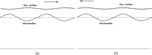
While in contrast to the long waves that we discussed earlier, the coupled westward propagating slow waves are in phase (see figure 5), the amplitude amplification at the thermocline is again very large (because $V$ is small and $d$ is large). For example, for the typical choice (38(38) $$\begin{array}{c}\hfill V\approx 0.015,W\approx 0.029,m=l\approx 0.33,n\approx 2,d\approx 33.\end{array}$$(38) ), this factor is about $1.5\times {10}^5$, meaning that even a spectacularly large internal wave of amplitude $40$ m is undetectable at the surface, since the amplitude of the corresponding surface wave is less than $0.001$ m.

Figure 5. The direction of propagation has an effect on the coupling of the surface and internal waves: (a) The eastward propagating coupled long waves are out of phase, with the crests/troughs of the internal wave located beneath the troughs/crests of the surface wave; (b) The westward propagating coupled long waves are in phase, with overlying wave crests/troughs.

6. Conclusions

We have presented a theory, based on simple principles, to explain the main features of wave-current interactions that are typical of the flows observed in the Pacific Ocean near the Equator. Our model uses, as its starting point, the inviscid, but rotational, equations of fluid motion, adjusted to include the $f$-plane approximation; these have been suitably non-dimensionalised and scaled in order to describe the perturbation of a background state. This background state has been chosen to accommodate all the salient features that are present: a wind-driven surface layer (westwards) and an EUC core that flows eastwards which has embedded in it a thermocline. The particular model for this background flow comprises a number of regions, each of which possesses constant vorticity – and it is this aspect of the model that makes significant headway possible. The process of linearisation simply allows the introduction of a linear wave system superimposed on the background flow, no other assumptions or simplifications being made. This results in the most general form of linear theory, and it is this that has been solved exactly (for harmonic waves).

Not surprisingly, the details turned out to be algebraically very involved, but otherwise the calculation is altogether routine. The use of a realistic background flow, and the minimal assumptions leading to the linearisation, have produced a theory from which it is possible to extract a significant amount of information, leading to ample opportunities to check with the available data, to make some predictions and to explain a number of the underlying processes. Indeed, our final expressions, in their greatest generality, are available for the analysis of many different, but similar, flows, and for any chosen wave length. We have elected to extract a few simple – but gratifyingly quite accurate – results by examining waves of short, intermediate and long wavelengths, coupled with suitable approximations driven by the sizes of some of the parameters in the problem. Of course, our theoretical approach cannot hope to reproduce, faithfully, all the fine detail of the very complicated dynamical processes involved in this oceanic flow, but we are able to provide some in-depth analysis which can be used to test and to make empirical predictions. To this end, our model incorporates many of the important factors that are necessary for the description of these flows, and also many adjustable parameters; we believe that we have provided firmly-based explanations for most of the fundamental processes that are relevant, and observed, in the motions in this equatorial region. In particular, we have found the following:

(1)	The significantly different behaviours of short, intermediate and long waves; here, short is relative to the mean depth of the thermocline, long is with respect to the ocean depth, while intermediate is long relative to the thermocline depth, but short relative to the ocean depth. By further approximating, taking advantage of the small change in density across the thermocline, and the size of the (non-dimensional) speeds in the background flow, we have obtained simple expressions for the speeds of these waves, and the strength of the coupling between the waves on the surface and those on the thermocline. We have seen that the character of these various relations changes markedly as the dependence on $r$ (a measure of the density difference), on the thicknesses of the various layers around the thermocline and on the speeds of the background flow, is different for different wavelengths. So, for example, the effect of short waves is confined to the near-surface layer, being very weakly coupled to the motion of the thermocline (section 4). On the other hand, for intermediate and long waves, the attenuation at the surface is considerable (section 5), so that waves of significant amplitude on the thermocline will not be visible at the surface (confirming many observations). Furthermore, our results are able to predict whether these coupled waves are in- or out-of-phase, depending on the wave regime. For all the above, we have obtained expressions that, in a simple form, provide a basis for testing our approach to this problem.
(2)	The extensive details of all the various modes and speeds of propagation – there are five for long waves, for example – have enabled us to predict that some wave speeds correspond to the appearance of critical layers in the flow. These can manifest themselves both above and below the thermocline, and there is now a growing body of observations that confirm their existence (and they are thought to be important in mixing processes below the surface). In the absence of critical layers, which is the more usual circumstance, then the wave motion is unidirectional, of course.
(3)	Our results show that there is a noticeable difference, both in terms of speeds and the coupling of the wave systems, between waves that propagate to the East and those that move westwards. The quantitative features of all the waves are summarised in table 1, and in table 2 we present the main properties of the observed equatorial current field.

Table 1. Main wave characteristics: The proposed theory predicts the speed and the amplitude ratio of the coupled waves at the surface and at the interface, while field data provide estimates for typical amplitudes of the oscillations of the thermocline and of the surface wave.

	Maximum speed	Typical amplitude	Pacific crossing time
	$({\mathrm{ms}}^{-1})$	(m)	(days)
Short eastward surface wave	12.2	3	12
Short eastward internal wave	12.2	0.015	12
Short westward surface wave	13.2	5	11
Short westward internal wave	13.2	0.025	11
Intermediate eastward surface wave	2.5	0.03	60
Intermediate eastward internal wave	2.5	5	60
Intermediate westward surface wave	0.5	0.03	300
Intermediate westward internal wave	0.5	5	300
Long and slow eastward surface wave	1.9	0.001	84
Long and slow eastward internal wave	1.9	20	84
Long and very slow eastward surface wave	0.12	0.001	1253
Long and very slow eastward internal wave	0.12	20	1253
Long and slow westward surface wave	0.5	0.0001	300
Long and slow westward internal wave	0.5	20	300

Table 2. Field data indicating the main characteristics of the underlying currents.

	Vertical range $\text{(m)}$	Maximum speed ${\text{(ms}}^{-1})$	Minimum speed ${\text{(ms}}^{-1})$
Westward surface drift	40	0.5	0
Eastward Equatorial Undercurrent	80	1	0

It is clear that further investigations will be necessary in order to uncover and describe more details of the dynamics of this flow environment. For example, an important issue in oceanographic studies is how thermal disturbances are propagated across the equatorial regions, driven by the underlying flow and the wave system. A first approach in this direction is offered in appendix E, but this is no more than an indication of what is possible, once we have a fairly complete and convincing theory of the wave-current interaction. We have shown that we can predict the appearance of critical layers; this type of flow is of particular interest, both theoretically and practically; we have briefly described the nature of critical layers, in this context, in appendix B, but this is worthy of more detailed attention.

Our development has aimed to describe the propagation of a harmonic wave against the background of a given current field; we have allowed any wavelength for this wave, but a more meaningful discussion would centre on the interaction between waves of different wavelength. Indeed, we can begin to address this in a very simple way, based directly on our analysis. We can consider the sum of two waves (at the surface, say), one short – the familiar surface gravity wave – and the other acting as a small-amplitude, long-wave modulation of this; this choice is fully covered by our theory. Of course, any proper interaction cannot be accessed through the work presented here; a more comprehensive and detailed analysis is required to accomplish this. Further, the waves that we have described, within the scenario that we envisage, are not expected to evolve over sufficiently long time or distance scales to the extent that nonlinearity becomes important. However, we must expect that nonlinearity will play a rôle in some wave phenomena – and there is some evidence for this – and so this is another avenue for exploration. Finally, an important extension of this work is to accommodate the $\mathit{\beta }$-plane approximation, and so incorporate some three-dimensionality (thus allowing for meridional variations), and also to permit the underlying flow to change (slowly) along the Equator. Many of the above extensions are currently under investigation.

Acknowledgements

The authors are grateful for helpful comments from the referees and from the editor. The support of the ERC Advanced Grant “Nonlinear studies of water flows with vorticity” is acknowledged.

Additional information

Funding

This work was supported by the ERC Advanced Grant ‘Nonlinear studies of water flows with vorticity’.

Notes

No potential conflict of interest was reported by the authors.

Appendix A

The equatorial current field

The theory developed in this paper requires the introduction of a suitable background flow, namely that given in (36(36) $$\begin{array}{c}\hfill U(z)=\left\{\begin{array}{cccc}-V-z(V+W)/(1-l)\hfill & \hfill \text{for}& \hfill -1+l& <z\le 0,\hfill \\ W\hfill & \hfill \text{for}& \hfill -1-m& <z\le -1+l,\hfill \\ W(z+n)/(n-1-m)\hfill & \hfill \text{for}& \hfill -n& <z\le -1-m,\hfill \\ 0\hfill & \hfill \text{for}& \hfill -d& \le z\le -n,\hfill \end{array}\right.\end{array}$$(36) ). Here, we present a simple two-dimensional linear model that explains the basic underlying qualitative mechanisms that give rise to this type of profile. The complexity of the dynamics implies that any model for the wind-induced current field in the equatorial region of the Pacific Ocean is bound to involve a trade-off between simplicity and realism/precision. We aim to find a balance between these two aspects, although we do not address the issue of quantitative accuracy – available data makes this almost impossible at this stage, due to the difficulties encountered in obtaining precise empirical estimates of the vertical eddy viscosity through experiments and measurements, and is beyond the scope of our discussion here.

To explain the origin of the shape of the equatorial current field, as described in section 2.3, we consider an initially calm setting in which a sudden westward wind-stress is applied to the ocean surface and then remains constant for a long time. In the absence of land boundaries, with a constant ocean depth and a uniform wind stress, no gradient of sea-surface elevation will occur (cf. Davies 2013) but the initial (constant) pressure at the ocean surface is altered and an underlying current field is generated. If the wind subsides – a feature that is observed, for example, in the context of the El Niño phenomenon (see also the discussion in appendix E) – then a rapid adjustment of the pressure at the surface to (constant) atmospheric pressure will occur. This resulting scenario is the one that is relevant to our theory and the choice of background profile, because, after the wind drops, the underlying current persists, its basic shape being captured by the background flow modelled by (36(36) $$\begin{array}{c}\hfill U(z)=\left\{\begin{array}{cccc}-V-z(V+W)/(1-l)\hfill & \hfill \text{for}& \hfill -1+l& <z\le 0,\hfill \\ W\hfill & \hfill \text{for}& \hfill -1-m& <z\le -1+l,\hfill \\ W(z+n)/(n-1-m)\hfill & \hfill \text{for}& \hfill -n& <z\le -1-m,\hfill \\ 0\hfill & \hfill \text{for}& \hfill -d& \le z\le -n,\hfill \end{array}\right.\end{array}$$(36) ). The issue is therefore: can we find a mechanism that generates a suitable background flow? Once this is in place, and the uniform wind drops, wave perturbations of this pure current background flow, studied in this paper, can be initiated by wind bursts. Of course, viscous theory is essential in explaining the genesis of the equatorial-current field induced by wind forcing, but in this paper we have pursued an inviscid study of equatorial wave-current interactions. This approach is appropriate since the values of the Reynolds numbers encountered in geophysical fluid dynamics are very large; see the discussion in Maslowe (1986).

Let us now describe the most basic framework for the interpretation of the wind-induced current field in the equatorial region of the Pacific ocean. Ignoring the detailed structure of the prevailing westward trade winds, we assume the wind stress to be uniform and consider the linearised equations for a forced steady-state flow, with a vanishing vertical-fluid-velocity component in the $f$-plane approximation:(106a) $$\begin{array}{cc}\hfill 0& {\displaystyle =-\frac{1}{\overline{\mathit{\rho }}}{\overline{P}}_{\overline{x}}+(\overline{\mathit{\nu }}{\overline{u}}_{\overline{z}}{)}_{\overline{z}},}\hfill \end{array}$$(106a) (106b) $$\begin{array}{cc}\hfill -2\overline{\mathit{\Omega }}\overline{u}& {\displaystyle =-\frac{1}{\overline{\mathit{\rho }}}{\overline{P}}_{\overline{z}}-\overline{g},}\hfill \end{array}$$(106b) (106c) $$\begin{array}{cc}\hfill {\overline{u}}_{\overline{x}}& =0,\hfill \end{array}$$(106c) in the frictional layer located beneath the surface $\overline{z}=0$ and above the thermocline $\overline{z}=-\overline{h}$, where $\overline{\mathit{\rho }}$ takes on the constant value ${\overline{\mathit{\rho }}}_0$. We assume the stress-shear relationship(A.1) $$\begin{array}{c}\hfill \overline{\mathit{\tau }}=\overline{\mathit{\rho }}\overline{\mathit{\nu }}{\overline{u}}_{\overline{z}},\end{array}$$(A.1)

for the wind-induced stress $\overline{\mathit{\tau }}(\overline{z})$ within the fluid, where $\overline{\mathit{\nu }}(\overline{z})$ is the vertical viscosity parameter (see McCreary 1985). In contrast to the classical model of uniform vertical viscosity, due to Stommel (1960), we assume that $\overline{\mathit{\nu }}(\overline{z})$ is depth-dependent. This assumption is consistent with measurements and was introduced by Cronin and Kessler (2009). Associated with (A.1) is the knowledge of the surface wind stress, ${\overline{\mathit{\tau }}}_0<0$,(A.2) $$\begin{array}{c}\hfill {\overline{\mathit{\rho }}}_0\overline{\mathit{\nu }}{\overline{u}}_{\overline{z}}={\overline{\mathit{\tau }}}_0\text{at}\overline{z}=0.\end{array}$$(A.2)

The considerations in Wenegrat et al. (2014) show that it is realistic to assume the validity of the relation $\overline{\mathit{\nu }}(0)=\overline{\mathit{\sigma }}|{\overline{\mathit{\tau }}}_0|$, for some (dimensional) constant $\overline{\mathit{\sigma }}$; thus (A.3(A.3) $$\begin{array}{c}\hfill {\overline{u}}_{\overline{z}}=-{\displaystyle \frac{1}{{\overline{\mathit{\rho }}}_0\overline{\mathit{\sigma }}}}\text{at}\overline{z}=0.\end{array}$$(A.3) ) becomes(A.3) $$\begin{array}{c}\hfill {\overline{u}}_{\overline{z}}=-{\displaystyle \frac{1}{{\overline{\mathit{\rho }}}_0\overline{\mathit{\sigma }}}}\text{at}\overline{z}=0.\end{array}$$(A.3)

Note that for moderate and high wind speeds, exceeding 5 ms${}^{-1}$, the surface wind stress $|{\overline{\mathit{\tau }}}_0|$ is a quadratic function of the wind speed:(A.4) $$\begin{array}{c}\hfill |{\overline{\mathit{\tau }}}_0|=c_D{\overline{\mathit{\rho }}}_a{\overline{U}}_w^2\end{array}$$(A.4) (in Nm${}^{-2}$), where ${\overline{U}}_w$ is the wind speed at 10 m above the sea surface, ${\overline{\mathit{\rho }}}_a$ is the density of air (about $1.22$ kgm${}^{-3}$) and $c_D\sim 0.0013$ is a (dimensionless) drag coefficient (see the discussion in Santiago-Mandujano and Firing (1990), Yelland and Taylor (1996)). This is relevant to the equatorial Pacific, where the average speed of the trade winds is typically about 7 ms${}^{-1}$. We also observe that (A.4(A.4) $$\begin{array}{c}\hfill |{\overline{\mathit{\tau }}}_0|=c_D{\overline{\mathit{\rho }}}_a{\overline{U}}_w^2\end{array}$$(A.4) ) shows that the shear at the surface does not depend on the wind speed. In the classical model, discussed in detail in the survey by Arthur (1953), one requires that the shear (and thus the stress) vanishes at the thermocline $\overline{z}=-\overline{h}$, nominally set as the centre of the EUC. We will also impose this condition, known to be realistic for the central Pacific region (cf. Cronin and Kessler 2009).

Differentiating the first equation in (A.1) with respect to the $\overline{z}$-variable and the second equation with respect to the $\overline{x}$-variable, their difference yields ${(\overline{\mathit{\nu }}{\overline{u}}_{\overline{z}})}_{\overline{z}\overline{z}}=0$ for $-\overline{h}<\overline{z}<0$. Taking into account the assumption of a vanishing shear at the thermocline, we see that(A.5) $$\begin{array}{c}\hfill \overline{\mathit{\nu }}{\overline{u}}_{\overline{z}}=\overline{A}(1+\frac{\overline{z}}{\overline{h}})\text{for}-\overline{h}<\overline{z}<0,\end{array}$$(A.5)

where $\overline{A}$ is some (dimensional) parameter; from (A.4(A.4) $$\begin{array}{c}\hfill |{\overline{\mathit{\tau }}}_0|=c_D{\overline{\mathit{\rho }}}_a{\overline{U}}_w^2\end{array}$$(A.4) ) we get(A.6) $$\begin{array}{c}\hfill \overline{A}=-{\displaystyle \frac{\overline{\mathit{\nu }}(0)}{{\overline{\mathit{\rho }}}_0\overline{\mathit{\sigma }}}}.\end{array}$$(A.6)

The surface drift $\overline{u}(0)$ is typically about 3$\%$ of the wind speed, with $|\overline{u}(0)|$ proportional to $\sqrt{|{\overline{\mathit{\tau }}}_0|}$ (see Wu 1975). Setting $\overline{u}(0)=-\overline{\mathit{\theta }}\sqrt{\overline{\mathit{\nu }}(0)}$ for some (dimensional) constant $\overline{\mathit{\theta }}$, from (A.6(A.6) $$\begin{array}{c}\hfill \overline{A}=-{\displaystyle \frac{\overline{\mathit{\nu }}(0)}{{\overline{\mathit{\rho }}}_0\overline{\mathit{\sigma }}}}.\end{array}$$(A.6) )–(A.7(A.7) $$\begin{array}{c}\hfill \overline{u}(\overline{z})=-\overline{\mathit{\theta }}\sqrt{\overline{\mathit{\nu }}(0)}+{\displaystyle \frac{\overline{\mathit{\nu }}(0)}{{\overline{\mathit{\rho }}}_0\overline{\mathit{\sigma }}}}{\int }_{\overline{z}}^0{\displaystyle \frac{1+(s/\overline{h})}{\overline{\mathit{\nu }}(s)}}\mathrm{d}s\text{for}-\overline{h}<\overline{z}\le 0.\end{array}$$(A.7) ) we obtain that(A.7) $$\begin{array}{c}\hfill \overline{u}(\overline{z})=-\overline{\mathit{\theta }}\sqrt{\overline{\mathit{\nu }}(0)}+{\displaystyle \frac{\overline{\mathit{\nu }}(0)}{{\overline{\mathit{\rho }}}_0\overline{\mathit{\sigma }}}}{\int }_{\overline{z}}^0{\displaystyle \frac{1+(s/\overline{h})}{\overline{\mathit{\nu }}(s)}}\mathrm{d}s\text{for}-\overline{h}<\overline{z}\le 0.\end{array}$$(A.7)

Let ${\overline{P}}_{\mathrm{a}tm}$ be the (constant) atmospheric pressure at the point $\overline{x}=0$, $\overline{z}=0$; if there is no wind, the pressure is atmospheric on the surface $\overline{z}=0$. We see that (A.1) and (A.8(A.8) $$\begin{array}{c}\hfill \overline{P}(\overline{x},\overline{z})=-{\displaystyle \frac{\overline{\mathit{\nu }}(0)}{\overline{\mathit{\sigma }}\overline{h}}}\overline{x}-{\overline{\mathit{\rho }}}_0\overline{g}\overline{z}-2{\overline{\mathit{\rho }}}_0\overline{\mathit{\Omega }}{\int }_{\overline{z}}^0\overline{u}(s)\mathrm{d}s+{\overline{P}}_{\mathrm{a}tm}\text{for}-\overline{h}<\overline{z}\le 0.\end{array}$$(A.8) ) yield(A.8) $$\begin{array}{c}\hfill \overline{P}(\overline{x},\overline{z})=-{\displaystyle \frac{\overline{\mathit{\nu }}(0)}{\overline{\mathit{\sigma }}\overline{h}}}\overline{x}-{\overline{\mathit{\rho }}}_0\overline{g}\overline{z}-2{\overline{\mathit{\rho }}}_0\overline{\mathit{\Omega }}{\int }_{\overline{z}}^0\overline{u}(s)\mathrm{d}s+{\overline{P}}_{\mathrm{a}tm}\text{for}-\overline{h}<\overline{z}\le 0.\end{array}$$(A.8)

In the deep layer beneath the thermocline, (A.1) has to be replaced by(115a) $$\begin{array}{cc}\hfill 0& {\displaystyle =-\frac{1}{(1+r){\overline{\mathit{\rho }}}_0}{\overline{P}}_{\overline{x}}+{(\overline{\mathit{\nu }}{\overline{u}}_{\overline{z}})}_{\overline{z}},}\hfill \end{array}$$(115a) (115b) $$\begin{array}{cc}\hfill -2\overline{\mathit{\Omega }}\overline{u}& {\displaystyle =-{\frac{1}{(1+r)\overline{\mathit{\rho }}}}_0{\overline{P}}_{\overline{z}}-\overline{g},}\hfill \end{array}$$(115b) (115c) $$\begin{array}{cc}\hfill {\overline{u}}_{\overline{x}}& =0.\hfill \end{array}$$(115c) The boundary conditions appropriate to the set (A.10) are the continuity of the horizontal velocity component, of the pressure and of the shear stress across the thermocline, together with the no-slip boundary condition(A.9) $$\begin{array}{c}\hfill \overline{u}=0\text{at the ocean bed}\overline{z}=-\overline{d}.\end{array}$$(A.9)

The equations in (A.10) show that$${(\overline{\mathit{\nu }}{\overline{u}}_{\overline{z}})}_{\overline{z}\overline{z}}=0$$

throughout the deep layer. Coupled with the assumption that the shear vanishes at the thermocline, this yields(A.10) $$\begin{array}{c}\hfill \overline{\mathit{\nu }}{\overline{u}}_{\overline{z}}=\overline{B}(1+\frac{\overline{z}}{\overline{h}})\text{for}-\overline{d}<\overline{z}<-\overline{h},\end{array}$$(A.10)

for some (dimensional) parameter $\overline{B}$. In view of (A.9(A.9) $$\begin{array}{c}\hfill \overline{u}=0\text{at the ocean bed}\overline{z}=-\overline{d}.\end{array}$$(A.9) ), (A.10), (A.12(A.12) $$\begin{array}{c}\hfill \overline{u}(\overline{z})=-{\displaystyle \frac{\overline{\mathit{\nu }}(0)}{(1+r){\overline{\mathit{\rho }}}_0\overline{\mathit{\sigma }}}}{\int }_{-\overline{d}}^{\overline{z}}{\displaystyle \frac{1+(s/\overline{h})}{\overline{\mathit{\nu }}(s)}}\mathrm{d}s\text{in the fluid region}-\overline{d}\le \overline{z}<-\overline{h},\end{array}$$(A.12) ), the continuity of the pressure across the thermocline shows that(A.11) $$\begin{array}{c}\hfill \overline{B}=-{\displaystyle \frac{\overline{\mathit{\nu }}(0)}{(1+r){\overline{\mathit{\rho }}}_0\overline{\mathit{\sigma }}}}.\end{array}$$(A.11)

Taking into account (A.11(A.11) $$\begin{array}{c}\hfill \overline{B}=-{\displaystyle \frac{\overline{\mathit{\nu }}(0)}{(1+r){\overline{\mathit{\rho }}}_0\overline{\mathit{\sigma }}}}.\end{array}$$(A.11) ), we deduce that(A.12) $$\begin{array}{c}\hfill \overline{u}(\overline{z})=-{\displaystyle \frac{\overline{\mathit{\nu }}(0)}{(1+r){\overline{\mathit{\rho }}}_0\overline{\mathit{\sigma }}}}{\int }_{-\overline{d}}^{\overline{z}}{\displaystyle \frac{1+(s/\overline{h})}{\overline{\mathit{\nu }}(s)}}\mathrm{d}s\text{in the fluid region}-\overline{d}\le \overline{z}<-\overline{h},\end{array}$$(A.12)

while$$\begin{array}{cc}\hfill \overline{P}(\overline{x},\overline{z})=& -{\displaystyle \frac{\overline{\mathit{\nu }}(0)}{\overline{\mathit{\sigma }}\overline{h}}}\overline{x}-{\overline{\mathit{\rho }}}_0\overline{g}[(1+r)\overline{z}+r\overline{h}]\hfill \\ \hfill & -2{\overline{\mathit{\rho }}}_0\overline{\mathit{\Omega }}{\int }_{-\overline{h}}^0\overline{u}(s)\mathrm{d}s-2{\overline{\mathit{\rho }}}_0\overline{\mathit{\Omega }}(1+r){\int }_{\overline{z}}^{-\overline{h}}\overline{u}(s)\mathrm{d}s+{\overline{P}}_{\mathrm{a}tm}\hfill \end{array}$$

below the thermocline, i.e. for $-\overline{d}\le \overline{z}\le -\overline{h}$. Due to (A.8(A.8) $$\begin{array}{c}\hfill \overline{P}(\overline{x},\overline{z})=-{\displaystyle \frac{\overline{\mathit{\nu }}(0)}{\overline{\mathit{\sigma }}\overline{h}}}\overline{x}-{\overline{\mathit{\rho }}}_0\overline{g}\overline{z}-2{\overline{\mathit{\rho }}}_0\overline{\mathit{\Omega }}{\int }_{\overline{z}}^0\overline{u}(s)\mathrm{d}s+{\overline{P}}_{\mathrm{a}tm}\text{for}-\overline{h}<\overline{z}\le 0.\end{array}$$(A.8) ) and (A.14(A.14) $$\begin{array}{c}\hfill \overline{\mathit{\nu }}(\overline{z})=\overline{\mathit{\nu }}(0)f(\overline{z}/\overline{d}),-\overline{d}\le \overline{z}\le 0,\end{array}$$(A.14) ), the relation(A.13) $$\begin{array}{c}\hfill -\overline{\mathit{\theta }}\sqrt{\overline{\mathit{\nu }}(0)}+{\displaystyle \frac{\overline{\mathit{\nu }}(0)}{{\overline{\mathit{\rho }}}_0\overline{\mathit{\sigma }}}}{\int }_{-\overline{h}}^0{\displaystyle \frac{1+(s/\overline{h})}{\overline{\mathit{\nu }}(s)}}\mathrm{d}s=-{\displaystyle \frac{\overline{\mathit{\nu }}(0)}{(1+r){\overline{\mathit{\rho }}}_0\overline{\mathit{\sigma }}}}{\int }_{-\overline{d}}^{-\overline{h}}{\displaystyle \frac{1+(s/\overline{h})}{\overline{\mathit{\nu }}(s)}}\mathrm{d}s\end{array}$$(A.13)

emerges from the continuity of $\overline{u}$ across the thermocline, both sides being equal to $\overline{u}(-\overline{h})$. Using (A.5(A.5) $$\begin{array}{c}\hfill \overline{\mathit{\nu }}{\overline{u}}_{\overline{z}}=\overline{A}(1+\frac{\overline{z}}{\overline{h}})\text{for}-\overline{h}<\overline{z}<0,\end{array}$$(A.5) ) and the fact that $\overline{\mathit{\nu }}(0)=\overline{\mathit{\sigma }}|{\overline{\mathit{\tau }}}_0|$, we see that the relation (A.15(A.15) $$\begin{array}{c}\hfill \mathit{\xi }=C{\int }_{-h}^0{\displaystyle \frac{1+(s/h)}{f(s/d)}}\mathrm{d}s+{\displaystyle \frac{C}{(1+r)}}{\int }_{-d}^{-h}{\displaystyle \frac{1+(s/h)}{f(s/d)}}\mathrm{d}s,\end{array}$$(A.15) ) expresses an implicit dependence of the thermocline depth $\overline{h}$ on the wind speed. We also observe that in the case $\overline{\mathit{\nu }}=\mathrm{constant}$, equations (A.8(A.8) $$\begin{array}{c}\hfill \overline{P}(\overline{x},\overline{z})=-{\displaystyle \frac{\overline{\mathit{\nu }}(0)}{\overline{\mathit{\sigma }}\overline{h}}}\overline{x}-{\overline{\mathit{\rho }}}_0\overline{g}\overline{z}-2{\overline{\mathit{\rho }}}_0\overline{\mathit{\Omega }}{\int }_{\overline{z}}^0\overline{u}(s)\mathrm{d}s+{\overline{P}}_{\mathrm{a}tm}\text{for}-\overline{h}<\overline{z}\le 0.\end{array}$$(A.8) ) and (A.14(A.14) $$\begin{array}{c}\hfill \overline{\mathit{\nu }}(\overline{z})=\overline{\mathit{\nu }}(0)f(\overline{z}/\overline{d}),-\overline{d}\le \overline{z}\le 0,\end{array}$$(A.14) ) imply that the velocity profile, $\overline{u}(\overline{z})$, is parabolic both above and below the thermocline (as in Stommel (1960)).

Glancing at (A.6(A.6) $$\begin{array}{c}\hfill \overline{A}=-{\displaystyle \frac{\overline{\mathit{\nu }}(0)}{{\overline{\mathit{\rho }}}_0\overline{\mathit{\sigma }}}}.\end{array}$$(A.6) ), (A.7(A.7) $$\begin{array}{c}\hfill \overline{u}(\overline{z})=-\overline{\mathit{\theta }}\sqrt{\overline{\mathit{\nu }}(0)}+{\displaystyle \frac{\overline{\mathit{\nu }}(0)}{{\overline{\mathit{\rho }}}_0\overline{\mathit{\sigma }}}}{\int }_{\overline{z}}^0{\displaystyle \frac{1+(s/\overline{h})}{\overline{\mathit{\nu }}(s)}}\mathrm{d}s\text{for}-\overline{h}<\overline{z}\le 0.\end{array}$$(A.7) ), (A.12(A.12) $$\begin{array}{c}\hfill \overline{u}(\overline{z})=-{\displaystyle \frac{\overline{\mathit{\nu }}(0)}{(1+r){\overline{\mathit{\rho }}}_0\overline{\mathit{\sigma }}}}{\int }_{-\overline{d}}^{\overline{z}}{\displaystyle \frac{1+(s/\overline{h})}{\overline{\mathit{\nu }}(s)}}\mathrm{d}s\text{in the fluid region}-\overline{d}\le \overline{z}<-\overline{h},\end{array}$$(A.12) ), (A.13(A.13) $$\begin{array}{c}\hfill -\overline{\mathit{\theta }}\sqrt{\overline{\mathit{\nu }}(0)}+{\displaystyle \frac{\overline{\mathit{\nu }}(0)}{{\overline{\mathit{\rho }}}_0\overline{\mathit{\sigma }}}}{\int }_{-\overline{h}}^0{\displaystyle \frac{1+(s/\overline{h})}{\overline{\mathit{\nu }}(s)}}\mathrm{d}s=-{\displaystyle \frac{\overline{\mathit{\nu }}(0)}{(1+r){\overline{\mathit{\rho }}}_0\overline{\mathit{\sigma }}}}{\int }_{-\overline{d}}^{-\overline{h}}{\displaystyle \frac{1+(s/\overline{h})}{\overline{\mathit{\nu }}(s)}}\mathrm{d}s\end{array}$$(A.13) ) and (A.15(A.15) $$\begin{array}{c}\hfill \mathit{\xi }=C{\int }_{-h}^0{\displaystyle \frac{1+(s/h)}{f(s/d)}}\mathrm{d}s+{\displaystyle \frac{C}{(1+r)}}{\int }_{-d}^{-h}{\displaystyle \frac{1+(s/h)}{f(s/d)}}\mathrm{d}s,\end{array}$$(A.15) ), we deduce that $\overline{u}$ attains its maximum $\overline{u}(-\overline{h})>0$ on the thermocline and its minimum $\overline{u}(0)=-\overline{\mathit{\theta }}\sqrt{\overline{\mathit{\nu }}(0)}<0$ on the free surface, being strictly increasing with depth above the thermocline and strictly decreasing below it, as plotted in figure A1 for a reasonable choice of the function $\overline{\mathit{\nu }}$ (see below). These considerations show that the choice of a piecewise linear current, as in the background flow (36(36) $$\begin{array}{c}\hfill U(z)=\left\{\begin{array}{cccc}-V-z(V+W)/(1-l)\hfill & \hfill \text{for}& \hfill -1+l& <z\le 0,\hfill \\ W\hfill & \hfill \text{for}& \hfill -1-m& <z\le -1+l,\hfill \\ W(z+n)/(n-1-m)\hfill & \hfill \text{for}& \hfill -n& <z\le -1-m,\hfill \\ 0\hfill & \hfill \text{for}& \hfill -d& \le z\le -n,\hfill \end{array}\right.\end{array}$$(36) ), captures the primary structure of the equatorial current system in the Pacific, where regular trade winds blow to the West.

Figure A1. Typical vertical profile of the equatorial current field in the Pacific region (in bold) and a piecewise linear approximation (dotted broken line). The horizontal axis points from West to East, along the Equator.

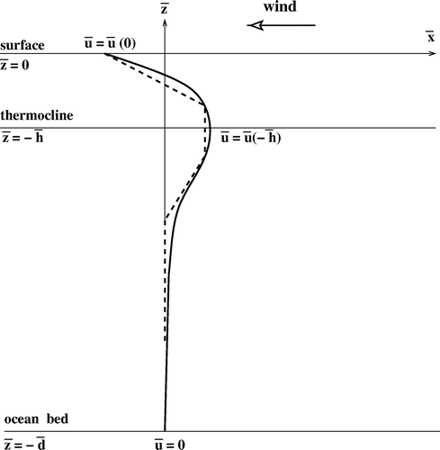
The microstructure measurements in Peters et al. (1988) and in Smyth et al. (1996) indicate that the vertical-eddy-viscosity-coefficient is depth-dependent. While for low wind speeds (below 3 ms${}^{-1}$) the behaviour presents anomalies due to surface tension effects, for moderate and high wind speeds a realistic choice is a viscosity coefficient of the form(A.14) $$\begin{array}{c}\hfill \overline{\mathit{\nu }}(\overline{z})=\overline{\mathit{\nu }}(0)f(\overline{z}/\overline{d}),-\overline{d}\le \overline{z}\le 0,\end{array}$$(A.14)

for a suitably chosen (non-dimensional) function $f$ that decays exponentially with depth in the layer above the thermocline (see Cronin and Kessler 2009). Expressing in (A.15(A.15) $$\begin{array}{c}\hfill \mathit{\xi }=C{\int }_{-h}^0{\displaystyle \frac{1+(s/h)}{f(s/d)}}\mathrm{d}s+{\displaystyle \frac{C}{(1+r)}}{\int }_{-d}^{-h}{\displaystyle \frac{1+(s/h)}{f(s/d)}}\mathrm{d}s,\end{array}$$(A.15) ) all dimensional variables in standard units of measure by setting $\overline{\mathit{\nu }}(0)={\mathit{\xi }}^2$ m${}^2$s${}^{-1}$ and otherwise dropping the overbar, we obtain, after some simple algebraic manipulation, the non-dimensional equation(A.15) $$\begin{array}{c}\hfill \mathit{\xi }=C{\int }_{-h}^0{\displaystyle \frac{1+(s/h)}{f(s/d)}}\mathrm{d}s+{\displaystyle \frac{C}{(1+r)}}{\int }_{-d}^{-h}{\displaystyle \frac{1+(s/h)}{f(s/d)}}\mathrm{d}s,\end{array}$$(A.15)

relating the variables $\mathit{\xi }>0$ and $h\in (0,d)$ by means of the fixed constants $C,d>0$ and the given function $f:[-1,0]\to (0,\infty )$, known to be strictly increasing on $[-h/d,0]$. Note that(A.16) $$\begin{array}{c}\hfill \frac{\mathrm{d}}{\mathrm{d}h}({\int }_{-h}^0{\displaystyle \frac{1+(s/h)}{f(s/d)}}\mathrm{d}s)=-\frac{1}{h^2}{\int }_{-h}^0{\displaystyle \frac{s\mathrm{d}s}{f(s/d)}}>0,\end{array}$$(A.16) (A.17) $$\begin{array}{c}\hfill \frac{\mathrm{d}}{\mathrm{d}h}({\int }_{-d}^{-h}{\displaystyle \frac{1+(s/h)}{f(s/d)}}\mathrm{d}s)=-\frac{1}{h^2}{\int }_{-d}^{-h}{\displaystyle \frac{s\mathrm{d}s}{f(s/d)}}>0,\end{array}$$(A.17)

while(A.18) $$\begin{array}{cc}\hfill {\displaystyle \frac{\mathrm{d}}{\mathrm{d}h}(\frac{1}{\sqrt{h}}{\int }_{-h}^0}& {\displaystyle \frac{1+(s/h)}{f(s/d)}}\mathrm{d}s)\hfill \\ \hfill & =-\frac{3}{2h^2\sqrt{h}}{\int }_{-h}^0{\displaystyle \frac{s\mathrm{d}s}{f(s/d)}}-\frac{1}{2h\sqrt{h}}{\int }_{-h}^0{\displaystyle \frac{\mathrm{d}s}{f(s/d)}}\hfill \\ \hfill & >-\frac{1}{2h^2\sqrt{h}}{\int }_{-h}^{-h/3}{\displaystyle \frac{3s\mathrm{d}s}{f(s/d)}}-\frac{1}{2h\sqrt{h}}{\int }_{-h}^0{\displaystyle \frac{\mathrm{d}s}{f(s/d)}}\hfill \\ \hfill & >\frac{1}{h\sqrt{h}}{\int }_{-h}^{-2h/3}{\displaystyle \frac{\mathrm{d}s}{f(s/d)}}+\frac{1}{2h\sqrt{h}}{\int }_{-2h/3}^{-h/3}{\displaystyle \frac{\mathrm{d}s}{f(s/d)}}-\frac{1}{2h\sqrt{h}}{\int }_{-h}^0{\displaystyle \frac{\mathrm{d}s}{f(s/d)}}\hfill \\ \hfill & =\frac{1}{2h\sqrt{h}}({\int }_{-h}^{-2h/3}{\displaystyle \frac{\mathrm{d}s}{f(s/d)}}-{\int }_{-h/3}^0{\displaystyle \frac{\mathrm{d}s}{f(s/d)}})>0,\hfill \end{array}$$(A.18)

and(A.19) $$\begin{array}{c}\hfill \frac{\mathrm{d}}{\mathrm{d}h}(\frac{1}{\sqrt{h}}{\int }_{-d}^{-h}{\displaystyle \frac{1+(s/h)}{f(s/d)}}\mathrm{d}s)=-\frac{1}{2h^2\sqrt{h}}{\int }_{-d}^{-h}{\displaystyle \frac{h+3s}{f(s/d)}}\mathrm{d}s>0.\end{array}$$(A.19)

In terms of the dimensional variables, comparing (A.17(A.17) $$\begin{array}{c}\hfill \frac{\mathrm{d}}{\mathrm{d}h}({\int }_{-d}^{-h}{\displaystyle \frac{1+(s/h)}{f(s/d)}}\mathrm{d}s)=-\frac{1}{h^2}{\int }_{-d}^{-h}{\displaystyle \frac{s\mathrm{d}s}{f(s/d)}}>0,\end{array}$$(A.17) ) with (A.15(A.15) $$\begin{array}{c}\hfill \mathit{\xi }=C{\int }_{-h}^0{\displaystyle \frac{1+(s/h)}{f(s/d)}}\mathrm{d}s+{\displaystyle \frac{C}{(1+r)}}{\int }_{-d}^{-h}{\displaystyle \frac{1+(s/h)}{f(s/d)}}\mathrm{d}s,\end{array}$$(A.15) ), we see that (A.18(A.18) $$\begin{array}{cc}\hfill {\displaystyle \frac{\mathrm{d}}{\mathrm{d}h}(\frac{1}{\sqrt{h}}{\int }_{-h}^0}& {\displaystyle \frac{1+(s/h)}{f(s/d)}}\mathrm{d}s)\hfill \\ \hfill & =-\frac{3}{2h^2\sqrt{h}}{\int }_{-h}^0{\displaystyle \frac{s\mathrm{d}s}{f(s/d)}}-\frac{1}{2h\sqrt{h}}{\int }_{-h}^0{\displaystyle \frac{\mathrm{d}s}{f(s/d)}}\hfill \\ \hfill & >-\frac{1}{2h^2\sqrt{h}}{\int }_{-h}^{-h/3}{\displaystyle \frac{3s\mathrm{d}s}{f(s/d)}}-\frac{1}{2h\sqrt{h}}{\int }_{-h}^0{\displaystyle \frac{\mathrm{d}s}{f(s/d)}}\hfill \\ \hfill & >\frac{1}{h\sqrt{h}}{\int }_{-h}^{-2h/3}{\displaystyle \frac{\mathrm{d}s}{f(s/d)}}+\frac{1}{2h\sqrt{h}}{\int }_{-2h/3}^{-h/3}{\displaystyle \frac{\mathrm{d}s}{f(s/d)}}-\frac{1}{2h\sqrt{h}}{\int }_{-h}^0{\displaystyle \frac{\mathrm{d}s}{f(s/d)}}\hfill \\ \hfill & =\frac{1}{2h\sqrt{h}}({\int }_{-h}^{-2h/3}{\displaystyle \frac{\mathrm{d}s}{f(s/d)}}-{\int }_{-h/3}^0{\displaystyle \frac{\mathrm{d}s}{f(s/d)}})>0,\hfill \end{array}$$(A.18) ) and (A.19(A.19) $$\begin{array}{c}\hfill \frac{\mathrm{d}}{\mathrm{d}h}(\frac{1}{\sqrt{h}}{\int }_{-d}^{-h}{\displaystyle \frac{1+(s/h)}{f(s/d)}}\mathrm{d}s)=-\frac{1}{2h^2\sqrt{h}}{\int }_{-d}^{-h}{\displaystyle \frac{h+3s}{f(s/d)}}\mathrm{d}s>0.\end{array}$$(A.19) ) imply(A.20) $$\begin{array}{c}\hfill [\overline{u}(-\overline{h})-\overline{u}(0)]\text{increases when}\overline{\mathit{\nu }}(0)\text{increases}\end{array}$$(A.20)

and(A.21) $$\begin{array}{c}\hfill \overline{u}(-\overline{h})\text{increases when}\overline{\mathit{\nu }}(0)\text{increases},\end{array}$$(A.21)

respectively. Similarly, (A.20(A.20) $$\begin{array}{c}\hfill [\overline{u}(-\overline{h})-\overline{u}(0)]\text{increases when}\overline{\mathit{\nu }}(0)\text{increases}\end{array}$$(A.20) ) and (A.21(A.21) $$\begin{array}{c}\hfill \overline{u}(-\overline{h})\text{increases when}\overline{\mathit{\nu }}(0)\text{increases},\end{array}$$(A.21) ) provide us with the monotonicity features(A.22) $$\begin{array}{c}\hfill [\overline{u}(-\overline{h})-\overline{u}(0)]/\sqrt{\overline{g}\overline{h}}\text{increases when}\overline{\mathit{\nu }}(0)\text{increases}\end{array}$$(A.22)

and(A.23) $$\begin{array}{c}\hfill \overline{u}(-\overline{h})/\sqrt{\overline{g}\overline{h}}\text{increases when}\overline{\mathit{\nu }}(0)\text{increases},\end{array}$$(A.23)

respectively, expressed in terms of the non-dimensionalisation described in (19(19) $$\begin{array}{cc}\hfill \overline{z}& =\overline{h}z,\overline{x}=\overline{h}x,\overline{t}=\overline{h}t/\sqrt{\overline{g}\overline{h}},\overline{\mathit{\eta }}=\overline{a}\mathit{\eta },\overline{H}=\overline{a}H,\hfill \\ \hfill (\overline{U}+\overline{u},\overline{w})& =\sqrt{\overline{g}\overline{h}}(U+u,w),\overline{P}+\overline{p}=\overline{{\mathit{\rho }}_0}\overline{g}\overline{h}(P+p),\hfill \end{array}$$(19) ). Finally, let us note that the monotonicity property:(A.24) $$\begin{array}{c}\hfill -\overline{u}(0)\text{increases when}\overline{\mathit{\nu }}(0)\text{increases},\end{array}$$(A.24)

follows at once since $\overline{u}(0)=-\overline{\mathit{\theta }}\sqrt{\overline{\mathit{\nu }}(0)}$. Consequently, for the background flow (36(36) $$\begin{array}{c}\hfill U(z)=\left\{\begin{array}{cccc}-V-z(V+W)/(1-l)\hfill & \hfill \text{for}& \hfill -1+l& <z\le 0,\hfill \\ W\hfill & \hfill \text{for}& \hfill -1-m& <z\le -1+l,\hfill \\ W(z+n)/(n-1-m)\hfill & \hfill \text{for}& \hfill -n& <z\le -1-m,\hfill \\ 0\hfill & \hfill \text{for}& \hfill -d& \le z\le -n,\hfill \end{array}\right.\end{array}$$(36) ), the strength of the westward surface drift $\overline{V}$ (respectively $V$), of the maximum speed of the EUC, $\overline{W}$ (respectively $W$), and of the total speed variation of the current field, $\overline{V}+\overline{W}$ (respectively $V+W$), all exhibit a monotonically increasing dependence on the speed of the generating wind. Moreover, the thermocline depth, $\overline{h}$ (respectively $h$), also presents this feature.

The development that we have presented here is intended as an indication of why we chose the particular background flow that we used for the analysis. The general form that we modelled is what is observed, but we thought that a brief outline of how we think it might come about would be useful. Of course, any careful and consistent discussion of the interaction between surface winds (and pressure) and the ocean, the rôle of surface and internal viscosities, and the timescales involved, is an immense task – and quite beyond the aims of the current work. The bottom line is that we need do no more than be given any (suitable) arbitrary background flow, and then proceed with our linear theory; in this context, the ideas presented in this appendix can be ignored.

Appendix B

Some considerations on real roots of quintics

Galois theory ensures that there is no general algebraic solution (in terms of radicals) which gives the roots to a quintic polynomial with arbitrary real coefficients. Nevertheless, if the coefficients are specified, the roots can be computed numerically to any desired degree of accuracy. To go beyond the limitations inherent in a case-by-case approach in order to draw some conclusions valid in a wider context, it is necessary to take advantage of the structural properties of the type of quintic under investigation. We present here some considerations valid for the quintic that underlies the dispersion relation for long waves (see section 5.2).

We write (103(103) $$\begin{array}{cc}\hfill (1-2\mathit{\Omega }c)\{(c+V)[d{(c-W)}^2+(1+m+n)cW-n{W}^2]-(1-l)c^2(V+W)\}& \hfill \\ \hfill =c^2{(c-W)}^2(c+V).& \hfill \end{array}$$(103) ) as(B.1) $$\begin{array}{c}\hfill \mathfrak{p}(c)=c^5+e_1{c}^4+e_2{c}^3+e_3{c}^2+e_{4}c+e_5,\end{array}$$(B.1)

where$$\begin{array}{cc}\hfill e_1=& -2W+V+2\mathit{\Omega }d,\hfill \\ \hfill e_2=& W^2-2VW-d+2\mathit{\Omega }\{W(l+m+n-2d)+V(d-1+l)\},\hfill \\ \hfill e_3=& d(2W-V)+V{W}^2-W(l+m+n)+(1-l)V\hfill \\ \hfill & +2\mathit{\Omega }\{VW(1+m+n-2d)+(d-n)W^2\},\hfill \\ \hfill e_4=& (n-d)W^2-VW[1+m+n-2d]+2\mathit{\Omega }\{(d-n)V{W}^2\},\hfill \\ \hfill e_5=& (n-d)V{W}^2.\hfill \end{array}$$

Since $\mathfrak{p}(c)\to \pm \infty$ as $c\to \pm \infty$ and$$\mathfrak{p}(-V)=(1-l)(V+W)V^2(1+2\mathit{\Omega }V)>0,\mathfrak{p}(0)=(n-d)V{W}^2<0,$$

we deduce that $\mathfrak{p}$ has at least three real roots: $c_1\in (-\infty ,-V)$, $c_2\in (-V,0)$ and $c_3\in (0,\infty )$. Since $\mathit{\Omega }\ll 1$, we have$$\begin{array}{cc}& e_1\approx -2W+V,\hfill \\ \hfill & e_2\approx W^2-2VW-d,\hfill \\ \hfill & e_3\approx d(2W-V)+V{W}^2-W(l+m+n)+(1-l)V,\hfill \\ \hfill & e_4\approx (n-d)W^2-VW[1+m+n-2d].\hfill \end{array}$$

Note that $V,W\ll 1$ while $l,m,n$ are all $\mathrm{O}(1)$. Since all five roots of $\mathfrak{p}$, in the complex palne, lie within the distance $1+{max}_{1\le j\le 4}|e_j|$ from the origin (see Prasolov 2004) then to find the approximate location of the real roots of (103(103) $$\begin{array}{cc}\hfill (1-2\mathit{\Omega }c)\{(c+V)[d{(c-W)}^2+(1+m+n)cW-n{W}^2]-(1-l)c^2(V+W)\}& \hfill \\ \hfill =c^2{(c-W)}^2(c+V).& \hfill \end{array}$$(103) ) we might let $\mathit{\Omega }\to 0$. This amounts to setting $\mathit{\Omega }=0$ in the coefficients of the polynomial $\mathfrak{p}$, so that we now have to locate the real roots of the polynomial(B.2) $$\begin{array}{cc}\hfill \mathfrak{q}(c)& =c^5-\{2W-V\}{c}^4-\{d-W^2+2VW\}{c}^3\hfill \\ \hfill & +\{d(2W-V)+V{W}^2-W(l+m+n)+(1-l)V\}{c}^2\hfill \\ \hfill & -\{dW(W-2V)-n{W}^2+VW[1+m+n]\}c-(d-n)V{W}^2.\hfill \end{array}$$(B.2)

We now take advantage of the inequality $V<W$ and of Descartes’ rule of signs, which states that the number of positive roots of the polynomial ${\sum }_{j=0}^n{a}_j{x}^j$, with real coefficients, does not exceed the number of sign changes in the sequence $a_0,a_1,\dots ,a_n$ (see Prasolov 2004). Irrespective of the sign of $(W-2V)$, we deduce that $\mathfrak{q}$ has at most three positive roots. Since the negative roots of $\mathfrak{q}(c)$ are the positive roots of $\mathfrak{q}(-c)$, there are at most two negative roots. Consequently, $\mathfrak{q}$ has precisely two negative roots: $c_1$ and $c_2$. Moreover, computing ${\mathfrak{q}}_{+}(c)=\mathfrak{q}(c-W)$:$$\begin{array}{c}\hfill {\mathfrak{q}}_{+}(c)\sim c^5-(7W-V)c^4-d{c}^3+d(2W-V)c^2-dW(W-2V)c-dV{W}^2\end{array}$$

and so Descartes’ sign rule applied to ${\mathfrak{q}}_{+}(-c)$ ensures that ${\mathfrak{q}}_{+}$ has at most two negative roots. Thus $\mathfrak{q}$ has at most two and therefore exactly two real roots smaller than $W$. Since $\mathfrak{q}(c)\to \infty$ for $c\to \infty$ and$$\mathfrak{q}(W)=-(l+m)W^2(V+W)<0,$$

we deduce that $\mathfrak{q}$ has at least one real root larger than $W$. We claim that there is just one real root larger than $W$. To prove this, let us write(B.3) $$\begin{array}{c}\hfill \mathfrak{q}(c)=(c^2-d){(c-W)}^2(c+V)+\widehat{\mathfrak{q}}(c),\end{array}$$(B.3)

where $\widehat{\mathfrak{q}}$ is the second-degree polynomial$$\widehat{\mathfrak{q}}(c)=\{-W(l+m+n)+(1-l)V\}{c}^2+\{n{W}^2-VW(1+m+n)\}c+nV{W}^2.$$

Since the relations$$\widehat{\mathfrak{q}}(0)=nV{W}^2>0,\widehat{\mathfrak{q}}(W)=-(l+m)W^2(V+W)<0,\widehat{\mathfrak{q}}(-\sqrt{d})<0,$$

ensure that $\widehat{\mathfrak{q}}(c)<0$ for $c<-\sqrt{d}$ and for $c>W$, a glance at the graph of the quintic polynomial $(c^2-d){(c-W)}^2(c+V)$, depicted in figure B1, confirms that $\mathfrak{q}$ has no roots in either of the intervals $(-\infty ,-\sqrt{d})$ and $(W,\sqrt{d})$. Were all roots of $\mathfrak{q}$ real, one would be located in the interval $(-\sqrt{d},-V)$, one in the interval $(-V,0)$, and three would have to be larger than $\sqrt{d}$; thus their sum would exceed $2\sqrt{d}-V\gg 2W-V$, which is impossible in view of Viète’s formula. Consequently two of the roots of $\mathfrak{q}$ are not real.

0

Figure B1. The graph of the quintic $(c^2-d){(c-W)}^2(c+V)$.

We conclude our discussion by deriving the asymptotic form of the three real roots of $\mathfrak{p}$. With $d\gg 1$ and $V,W\ll 1$ such that $dW$ and $dV$ are both $\mathrm{O}(1)$, the fact that the polynomial (B.2(B.2) $$\begin{array}{cc}\hfill \mathfrak{q}(c)& =c^5-\{2W-V\}{c}^4-\{d-W^2+2VW\}{c}^3\hfill \\ \hfill & +\{d(2W-V)+V{W}^2-W(l+m+n)+(1-l)V\}{c}^2\hfill \\ \hfill & -\{dW(W-2V)-n{W}^2+VW[1+m+n]\}c-(d-n)V{W}^2.\hfill \end{array}$$(B.2) ) has only one relatively large coefficient, namely that of the cubic term, yields(B.4) $$\begin{array}{c}\hfill c_1\approx -\sqrt{d},c_3\approx \sqrt{d}\end{array}$$(B.4) (see also the discussion in Pakdemirli and Sari (2013)). As for $c_2\in (-V,0)$, since$$|\mathfrak{q}(0)|=(d-n)V{W}^2\gg (1-l)V^2(V+W)=\mathfrak{q}(-V),$$

we expect $c_2\approx -V$. Set $c_2=-V+\mathit{\gamma }$ with $\mathit{\gamma }\in (0,V)$. From $\mathfrak{q}(c_2)=0$, using (B.3(B.3) $$\begin{array}{c}\hfill \mathfrak{q}(c)=(c^2-d){(c-W)}^2(c+V)+\widehat{\mathfrak{q}}(c),\end{array}$$(B.3) ), we get, retaining the relevant dominant terms,$$\begin{array}{cc}& [-3d{V}^2-2d(2W-V)V-dW(W-2V)]\mathit{\gamma }\hfill \\ \hfill & +V^2[-W(l+m+n)+(1-l)V]\hfill \\ \hfill & +V[-n{W}^2+VW(1+m+n)]+nV{W}^2\sim 0.\hfill \end{array}$$

Thus$$\mathit{\gamma }\sim {\displaystyle \frac{(1-l)V^2}{d(V+W)}},$$

so that(B.5) $$\begin{array}{c}\hfill c_2\sim -V+{\displaystyle \frac{(1-l)V^2}{d(V+W)}}.\end{array}$$(B.5)

Appendix C

Critical layers

If the speed of the coupled surface and internal waves, $c$, is such that $-V<c<W$, then a critical layer exists in Region I. Moreover, if $0<c<W$, then there is a second, corresponding critical layer in Region IV. We analyse the situation for the critical layer in Region I, the considerations for Region IV being analogous.

The non-dimensional, scaled equations in Region I are$$\begin{array}{cc}\hfill u_t+(-V-{\mathit{\gamma }}_{+}z+\mathit{\epsilon }u)u_x+w(-{\mathit{\gamma }}_{+}+\mathit{\epsilon }{u}_z)+2\mathit{\Omega }w=& -p_x,\hfill \\ \hfill w_t+(-V-{\mathit{\gamma }}_{+}z+\mathit{\epsilon }u)w_x+\mathit{\epsilon }w{w}_z-2\mathit{\Omega }u=& -p_z,\hfill \\ \hfill u_x+w_z=& 0;\hfill \end{array}$$

see (28)–(35(35) $$\begin{array}{cccc}\hfill w=& 0\text{on}\hfill & \hfill z=& -d.\hfill \end{array}$$(35) ) and (36(36) $$\begin{array}{c}\hfill U(z)=\left\{\begin{array}{cccc}-V-z(V+W)/(1-l)\hfill & \hfill \text{for}& \hfill -1+l& <z\le 0,\hfill \\ W\hfill & \hfill \text{for}& \hfill -1-m& <z\le -1+l,\hfill \\ W(z+n)/(n-1-m)\hfill & \hfill \text{for}& \hfill -n& <z\le -1-m,\hfill \\ 0\hfill & \hfill \text{for}& \hfill -d& \le z\le -n,\hfill \end{array}\right.\end{array}$$(36) ). We introduce the characteristic $\mathit{\xi }=x-ct$ associated with this wave motion to give(C.1) $$\begin{array}{cc}\hfill (-c-V-{\mathit{\gamma }}_{+}z+\mathit{\epsilon }u)u_{\mathit{\xi }}+w(-{\mathit{\gamma }}_{+}+\mathit{\epsilon }{u}_z)+2\mathit{\Omega }w=& -p_{\mathit{\xi }},\hfill \end{array}$$(C.1) (C.2) $$\begin{array}{cc}\hfill (-c-V-{\mathit{\gamma }}_{+}z+\mathit{\epsilon }u)w_{\mathit{\xi }}+\mathit{\epsilon }w{w}_z-2\mathit{\Omega }u=& -p_z,\hfill \end{array}$$(C.2) (C.3) $$\begin{array}{cc}\hfill u_{\mathit{\xi }}+w_z=& 0.\hfill \end{array}$$(C.3)

Now the solution valid away from the critical layer (in Region I), based on the linear problem, can be expressed in terms of the stream function $\mathit{\psi }(\mathit{\xi },z)$, determined up to a constant by$${\mathit{\psi }}_{\mathit{\xi }}=-\mathit{\epsilon }w\text{and}{\mathit{\psi }}_z=U+\mathit{\epsilon }u.$$

We have, for $\mathit{\epsilon }\to 0$,$$\begin{array}{cc}& {\mathit{\psi }}_{\mathit{\xi }}\sim -\mathit{\epsilon }(A{\mathrm{e}}^{kz}+B{\mathrm{e}}^{-kz})sin(k\mathit{\xi }),\hfill \\ \hfill & {\mathit{\psi }}_z\sim -V-{\mathit{\gamma }}_{+}z+\mathit{\epsilon }(A{\mathrm{e}}^{kz}-B{\mathrm{e}}^{-kz})cos(k\mathit{\xi }),\hfill \end{array}$$

and so$$\mathit{\psi }\sim -Vz-{\displaystyle \frac{{\mathit{\gamma }}_{+}}{2}}{z}^2+\mathit{\epsilon }{\displaystyle \frac{A{\mathrm{e}}^{kz}+B{\mathrm{e}}^{-kz}}{k}}cos(k\mathit{\xi }).$$

We define $z_c$, the mid-line of the critical layer, by $c+V+{\mathit{\gamma }}_{+}{z}_c=0$; writing $z=z_c+\mathit{\delta }Z$ gives$$\begin{array}{cc}\hfill \mathit{\psi }\sim -V{z}_c-{\displaystyle \frac{{\mathit{\gamma }}_{+}}{2}}{z}_c^2& -\mathit{\delta }(V+{\mathit{\gamma }}_{+}{z}_c)Z-{\mathit{\delta }}^2{\displaystyle \frac{{\mathit{\gamma }}_{+}}{2}}{Z}^2\hfill \\ \hfill & +\mathit{\epsilon }{\displaystyle \frac{1}{k}}(A{\mathrm{e}}^{k{z}_c}+B{\mathrm{e}}^{-k{z}_c}+\mathrm{O}(\mathit{\delta }))cos(k\mathit{\xi }).\hfill \end{array}$$

We now introduce the stream function $\widehat{\mathit{\psi }}(\mathit{\xi },z)$ in the moving frame, defined up to an additive constant by$${\widehat{\mathit{\psi }}}_z=U+\mathit{\epsilon }u-c\text{and}{\widehat{\mathit{\psi }}}_{\mathit{\xi }}=-\mathit{\epsilon }w.$$

Thus we obtain(C.4) $$\begin{array}{c}\hfill \widehat{\mathit{\psi }}+(V+c)z_c+{\displaystyle \frac{{\mathit{\gamma }}_{+}}{2}}{z}_c^2\sim -{\mathit{\delta }}^2{\displaystyle \frac{{\mathit{\gamma }}_{+}}{2}}{Z}^2+\mathit{\epsilon }{\displaystyle \frac{1}{k}}(A{\mathrm{e}}^{k{z}_c}+B{\mathrm{e}}^{-k{z}_c})cos(k\mathit{\xi }),\end{array}$$(C.4)

an asymptotic representation which breaks down in the classical way: where $\mathit{\delta }=O(\sqrt{\mathit{\epsilon }})$. On the basis of this breakdown of the asymptotic expansion near the critical layer, we introduce the relevant variables valid in the neighbourhood of this critical layer. We write$$z=z_c+\sqrt{\mathit{\epsilon }}Z\text{and}u={\displaystyle \frac{1}{\sqrt{\mathit{\epsilon }}}}\tilde{U}(\mathit{\xi },Z;\mathit{\epsilon }),$$$$\text{with}w=\tilde{W}(\mathit{\xi },Z;\mathit{\epsilon }),p=\tilde{P}(\mathit{\xi },Z;\mathit{\epsilon }),$$

and we note that $c+V+{\mathit{\gamma }}_{+}z={\mathit{\gamma }}_{+}\sqrt{\mathit{\epsilon }}Z$. The governing equations (C.1(C.1) $$\begin{array}{cc}\hfill (-c-V-{\mathit{\gamma }}_{+}z+\mathit{\epsilon }u)u_{\mathit{\xi }}+w(-{\mathit{\gamma }}_{+}+\mathit{\epsilon }{u}_z)+2\mathit{\Omega }w=& -p_{\mathit{\xi }},\hfill \end{array}$$(C.1) )–(C.3(C.3) $$\begin{array}{cc}\hfill u_{\mathit{\xi }}+w_z=& 0.\hfill \end{array}$$(C.3) ) near the critical layer in Region I therefore become$$\begin{array}{cc}\hfill (-{\mathit{\gamma }}_{+}Z+\tilde{U}){\tilde{U}}_{\mathit{\xi }}+\tilde{W}(-{\mathit{\gamma }}_{+}+{\tilde{U}}_Z)+2\mathit{\Omega }\tilde{W}=& -{\tilde{P}}_{\mathit{\xi }},\hfill \\ \hfill \mathit{\epsilon }\{(-{\mathit{\gamma }}_{+}Z+\tilde{U}){\tilde{W}}_{\mathit{\xi }}+\tilde{W}{\tilde{W}}_Z\}-2\mathit{\Omega }\tilde{U}=& -{\tilde{P}}_X,\hfill \\ \hfill {\tilde{U}}_{\mathit{\xi }}+{\tilde{W}}_Z=& 0.\hfill \end{array}$$

To proceed, we introduce the stream function $\mathrm{\Psi }$ appropriate to this region, so that $\tilde{U}={\mathrm{\Psi }}_Z$ and $\tilde{W}=-{\mathrm{\Psi }}_{\mathit{\xi }}$, and then the leading-order problem here, as $\mathit{\epsilon }\to 0$, is given by$$\begin{array}{cc}\hfill ({\mathrm{\Psi }}_Z-{\mathit{\gamma }}_{+}Z){\mathrm{\Psi }}_{Z\mathit{\xi }}-{\mathrm{\Psi }}_{\mathit{\xi }}(-{\mathit{\gamma }}_{+}+{\mathrm{\Psi }}_{ZZ})-2\mathit{\Omega }{\mathrm{\Psi }}_{\mathit{\xi }}=& -{\tilde{P}}_{\mathit{\xi }},\hfill \\ \hfill 2\mathit{\Omega }{\mathrm{\Psi }}_Z=& {\tilde{P}}_Z.\hfill \end{array}$$

Differentiating the first equation with respect to the $Z$-variable yields$$({\mathrm{\Psi }}_Z-{\mathit{\gamma }}_{+}Z){({\mathrm{\Psi }}_{ZZ})}_{\mathit{\xi }}-{\mathrm{\Psi }}_{\mathit{\xi }}{({\mathrm{\Psi }}_{ZZ})}_Z=0.$$

This means that the gradients of the functions $(\mathrm{\Psi }-{\mathit{\gamma }}_{+}{Z}^2/2)$ and ${\mathrm{\Psi }}_{ZZ}$ are aligned, so that ${\mathrm{\Psi }}_{ZZ}$ and $(\mathrm{\Psi }-{\mathit{\gamma }}_{+}{Z}^2/2)$ must be functionally dependent; see the discussion in Newns (1967). Due to (C.4(C.4) $$\begin{array}{c}\hfill \widehat{\mathit{\psi }}+(V+c)z_c+{\displaystyle \frac{{\mathit{\gamma }}_{+}}{2}}{z}_c^2\sim -{\mathit{\delta }}^2{\displaystyle \frac{{\mathit{\gamma }}_{+}}{2}}{Z}^2+\mathit{\epsilon }{\displaystyle \frac{1}{k}}(A{\mathrm{e}}^{k{z}_c}+B{\mathrm{e}}^{-k{z}_c})cos(k\mathit{\xi }),\end{array}$$(C.4) ), the appropriate solution must match to$$-{\displaystyle \frac{{\mathit{\gamma }}_{+}}{2}}{Z}^2+{\displaystyle \frac{1}{k}}(A{\mathrm{e}}^{k{z}_c}+B{\mathrm{e}}^{-k{z}_c})cos(k\mathit{\xi })$$

for $Z=\mathrm{O}(1/\sqrt{\mathit{\epsilon }})$. Thus ${\mathrm{\Psi }}_{ZZ}\approx -{\mathit{\gamma }}_{+}$ throughout, and the stream function in the moving frame near the critical layer is therefore$$\mathrm{\Psi }\approx -{\displaystyle \frac{{\mathit{\gamma }}_{+}}{2}}{Z}^2+{\displaystyle \frac{1}{k}}(A{\mathrm{e}}^{k{z}_c}+B{\mathrm{e}}^{-k{z}_c})cos(k\mathit{\xi }).$$

The streamlines are then expressed as$$-{\displaystyle \frac{{\mathit{\gamma }}_{+}}{2}}{Z}^2+{\displaystyle \frac{1}{k}}(A{\mathrm{e}}^{k{z}_c}+B{\mathrm{e}}^{-k{z}_c})cos(k\mathit{\xi })=\text{constant}.$$

This family of streamlines recovers the classical Kelvin cat’s-eyes; see figure C1.

0

Figure C1. In the moving frame, the critical points of the stream function are surrounded by closed streamlines (Kelvin’s “cat’s eye” flow pattern). The critical layer, depicted by the dashed curve, is the hallmark of flow reversal, the flow being uni-directional away from the critical layer.

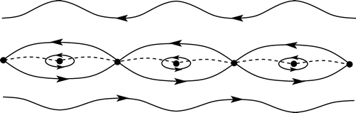
The condition for the existence of a critical layer in Region I is(C.5) $$\begin{array}{c}\hfill z_c=-(c+V)/{\mathit{\gamma }}_{+}>-1+l.\end{array}$$(C.5)

For short waves, using (66(66) $$\begin{array}{c}\hfill c\sim -V\pm \sqrt{{\displaystyle \frac{1+2\mathit{\Omega }V}{k}}}\text{as}k\to \infty .\end{array}$$(66) ), we see that (C.5(C.5) $$\begin{array}{c}\hfill z_c=-(c+V)/{\mathit{\gamma }}_{+}>-1+l.\end{array}$$(C.5) ) amounts to $\sqrt{k}>1/(V+W)$. In physical variables, this corresponds to the requirement that the wavelength $\overline{L}$ satisfies $\overline{L}<2\mathit{\pi }{(\overline{V}+\overline{W})}^2/\overline{g}$. Since, typically, this amounts to very small wavelengths (a few metres at most), we conclude that short waves do not generate critical layers in Region I. However, critical layers in Region I will arise due to westward propagating long waves with speeds close to $V$. In this case, (B.5(B.5) $$\begin{array}{c}\hfill c_2\sim -V+{\displaystyle \frac{(1-l)V^2}{d(V+W)}}.\end{array}$$(B.5) ) from appendix B transforms (C.5(C.5) $$\begin{array}{c}\hfill z_c=-(c+V)/{\mathit{\gamma }}_{+}>-1+l.\end{array}$$(C.5) ) into the condition $V^2<d(1-l)$, which is clearly satisfied for the typical choice (38(38) $$\begin{array}{c}\hfill V\approx 0.015,W\approx 0.029,m=l\approx 0.33,n\approx 2,d\approx 33.\end{array}$$(38) ). Field evidence for critical layers above the thermocline is provided in Smyth et al. (2011).

We also point out that long, single harmonic waves propagating eastward at speeds $c<W$ will always generate critical layers in Region IV. To see this, it suffices to note that the level $z_c$ of the critical layer in Region IV is defined by the solution to the equation$$-c+W(z_c+n)/(n-1-m)=0,$$

and for $c\in (0,W)$ with $W<1$, we have $z_c\in (-n,-1-m)$. Consequently, long waves propagating eastwards at speeds $\overline{c}<\overline{W}$ will generate critical layers beneath the thermocline.

Appendix D

The Burns condition for equatorial shear flows

The equations(142a) $$\begin{array}{cc}\hfill u_t+U(z)u_x+w{U}^{\prime }(z)+2\mathit{\Omega }w=& -p_x,\hfill \end{array}$$(142a) (142b) $$\begin{array}{cc}\hfill w_t+U(z)w_x-2\mathit{\Omega }u=& -p_z,\hfill \end{array}$$(142b) in the region $(-d<z<0)$, coupled with(D.1) $$\begin{array}{ccccc}\hfill u_x+w_z=& 0\hfill & \hfill \text{in}& -d<z\hfill & <0,\end{array}$$(D.1) (D.2) $$\begin{array}{ccccc}\hfill u_z-w_x=& 0\hfill & \hfill \text{in}& -d<z\hfill & <0,\end{array}$$(D.2) (D.3) $$\begin{array}{ccccc}\hfill p=& (1+2\mathit{\Omega }V)\mathit{\eta }\hfill & \hfill \text{on}& z\hfill & =0,\end{array}$$(D.3) (D.4) $$\begin{array}{ccccc}\hfill w=& {\mathit{\eta }}_t-V{\mathit{\eta }}_x\hfill & \hfill \text{on}& z\hfill & =0,\end{array}$$(D.4) (D.5) $$\begin{array}{ccccc}\hfill w=& 0\hfill & \hfill \text{on}& z\hfill & =-d,\end{array}$$(D.5)

are the leading order (linear) equations obtained in the limit $r\to 0$ of (39)–(47(47) $$\begin{array}{ccccc}\hfill w=& 0\hfill & \hfill \text{on}& z\hfill & =-d,\end{array}$$(47) ), as required in the long-wave approximation of our problem – see the discussion in section 5.2. In particular, in the limit $r\to 0$ the presence of the thermocline is neglected. To investigate the system (D.1)–(D.6(D.6) $$\begin{array}{ccccc}\hfill u_{\mathit{\xi }}+w_z=& 0\hfill & \hfill \text{in}& -d<z\hfill & <0,\end{array}$$(D.6) ), we first introduce a travelling wave: with $\mathit{\xi }=x-ct$, we have(148a) $$\begin{array}{cc}\hfill [U(z)-c]u_{\mathit{\xi }}+wU{}^{\prime }(z)+2\mathit{\Omega }w& =-p_{\mathit{\xi }},\hfill \end{array}$$(148a) (148b) $$\begin{array}{cc}\hfill [U(z)-c]w_{\mathit{\xi }}-2\mathit{\Omega }u& =-p_z,\hfill \end{array}$$(148b) in the region $(-d<z<0)$, coupled with(D.6) $$\begin{array}{ccccc}\hfill u_{\mathit{\xi }}+w_z=& 0\hfill & \hfill \text{in}& -d<z\hfill & <0,\end{array}$$(D.6) (D.7) $$\begin{array}{ccccc}\hfill u_z-w_{\mathit{\xi }}=& 0\hfill & \hfill \text{in}& -d<z\hfill & <0,\end{array}$$(D.7) (D.8) $$\begin{array}{ccccc}\hfill p=& (1+2\mathit{\Omega }V)\mathit{\eta }\hfill & \hfill \text{on}& z\hfill & =0,\end{array}$$(D.8) (D.9) $$\begin{array}{ccccc}\hfill w=& -(c+V){\mathit{\eta }}_{\mathit{\xi }}\hfill & \hfill \text{on}& z\hfill & =0,\end{array}$$(D.9) (D.10) $$\begin{array}{ccccc}\hfill w=& 0\hfill & \hfill \text{on}& z\hfill & =-d.\end{array}$$(D.10)

Now we impose the condition for long waves, e.g. we seek a solution with a $(\mathit{\xi },z)$-dependence in the form $(k\mathit{\xi },z)$ and let $k\to 0$. That is, we set$$u=\tilde{u}(\mathit{\chi },z),w=k\tilde{w}(\mathit{\chi },z),\mathit{\eta }=\tilde{\mathit{\eta }}(\mathit{\chi },z),p=\tilde{p}(\mathit{\chi },z)\text{with}\mathit{\chi }=k\mathit{\xi };$$

the different scaling of $w$ being imposed to ensure the consistency of the equation of mass conservation, (D.8(D.8) $$\begin{array}{ccccc}\hfill p=& (1+2\mathit{\Omega }V)\mathit{\eta }\hfill & \hfill \text{on}& z\hfill & =0,\end{array}$$(D.8) ), in the new variables $(\mathit{\chi },z)$. This gives, at leading order as $k\to 0$,(154a) $$\begin{array}{cc}\hfill [U(z)-c]{\tilde{u}}_{\mathit{\chi }}+\tilde{w}{U}^{\prime }(z)+2\mathit{\Omega }\tilde{w}=& -p_{\mathit{\xi }},\hfill \end{array}$$(154a) (154b) $$\begin{array}{cc}\hfill 2\mathit{\Omega }\tilde{u}=& -{\tilde{p}}_z,\hfill \end{array}$$(154b) in the region $(-d<z<0)$, coupled with(D.11) $$\begin{array}{ccccc}\hfill {\tilde{u}}_{\mathit{\chi }}+{\tilde{w}}_z=& 0\hfill & \hfill \text{in}& -d<z\hfill & <0,\end{array}$$(D.11) (D.12) $$\begin{array}{ccccc}\hfill {\tilde{u}}_z=& 0\hfill & \hfill \text{in}& -d<z\hfill & <0,\end{array}$$(D.12) (D.13) $$\begin{array}{ccccc}\hfill \tilde{p}=& (1+2\mathit{\Omega }V)\tilde{\mathit{\eta }}\hfill & \hfill \text{on}& z\hfill & =0,\end{array}$$(D.13) (D.14) $$\begin{array}{ccccc}\hfill \tilde{w}=& -(c+V){\tilde{\mathit{\eta }}}_{\mathit{\chi }}\hfill & \hfill \text{on}& z\hfill & =0,\end{array}$$(D.14) (D.15) $$\begin{array}{ccccc}\hfill \tilde{w}=& 0\hfill & \hfill \text{on}& z\hfill & =-d.\end{array}$$(D.15)

Thus$$\tilde{p}(\mathit{\chi },z)=2\mathit{\Omega }z\tilde{u}(\mathit{\chi })+(1+2\mathit{\Omega }V)\tilde{\mathit{\eta }}(\mathit{\chi }),\tilde{w}(\mathit{\xi },z)=-z{\tilde{u}}_{\mathit{\chi }}(\mathit{\chi })-(c+V){\tilde{\mathit{\eta }}}_{\mathit{\chi }}(\mathit{\chi }),$$

and so we get$$d{\tilde{u}}_{\mathit{\chi }}=(c+V){\tilde{\mathit{\eta }}}_{\mathit{\chi }}$$

and$$[U(z)-c]-(z+d)U^{\prime }(z)={\displaystyle \frac{(2\mathit{\Omega }c-1)d}{c+V}}.$$

Multiplying both sides by $1/{[U(z)-c]}^2$ and integrating on $[-d,0]$, this produces(D.16) $$\begin{array}{c}\hfill 1=(1-2\mathit{\Omega }c){\int }_{-d}^0{\displaystyle \frac{\mathrm{d}z}{{[U(z)-c]}^2}},\end{array}$$(D.16)

which is the Burns condition for this problem. For $\mathit{\Omega }=0$ in (D.19(13) $$\begin{array}{c}\hfill {\overline{u}}_{\overline{x}}+{\overline{w}}_{\overline{z}}=0,\end{array}$$(13) ) we recover the classical result given by Burns (1953), relating the speed of propagation of long water waves to the background-current-velocity distribution.

Appendix E

Propagation of thermal disturbances

Small variations (of the order of 1 ${}^{\circ }$C) in the magnitude of the sea surface temperature in the equatorial Pacific, where the mean sea surface temperature exceeds 27 ${}^{\circ }$C, can result in dramatic shifts in weather patterns (cf. Palmer and Mansfield 1984). In this process, the EUC variability, due to anomalies in the equatorial zonal wind, leads to wave-induced changes in the entire equatorial oceanic circulation. These seasonal variations are strongly linked to the El Niño Southern Oscillation (ENSO) and have an impact on the global climate (see Kessler 2002). We now briefly discuss the rôle played by interactions between ocean waves and the EUC towards the redistribution of heat in the equatorial Pacific. While both vertical and horizontal heat transport influence the thermal structure of the ocean, we do not aim to provide a comprehensive discussion here. For simplicity, and since this process is often dominant in the variability of the sea-surface temperature (cf. the discussion in Cronin and McPhaden (1997)), we restrict our attention to the eastward heat advection. Note that the rate of heat energy transport through the surface responds mainly to changes in the sea-surface temperature (see Haney 1971, Boccaletti et al. 2004, Boccaletti 2005, Wallcraft et al. 2008), with the dimensional ocean-atmosphere heat flux $\overline{Q}$ well-approximated as(E.1) $$\begin{array}{c}\hfill \overline{Q}=\overline{\mathit{\alpha }}({\overline{T}}^{\ast }-\overline{T}),\end{array}$$(E.1)

in which $\overline{T}$ is the sea-surface temperature, while typical values of the relaxation coefficient $\overline{\mathit{\alpha }}$, and of the threshold atmospheric temperature ${\overline{T}}^{\ast }$ for the equatorial Pacific, are about 50 Wm${}^{-2}$ C${}^{-1}$ and $27.5^{\circ }$C, respectively (cf. Philander 1989). A negative sign in (E.1(E.1) $$\begin{array}{c}\hfill \overline{Q}=\overline{\mathit{\alpha }}({\overline{T}}^{\ast }-\overline{T}),\end{array}$$(E.1) ) implies upward heat flux, so that the effect of a sea-surface temperature in excess of ${\overline{T}}^{\ast }$ is a transfer of heat from the ocean into the atmosphere.

We assume that the convection of temperature changes, $T(x,z,t)$, due to the flow of the ocean, driven by the propagation of waves, is governed by the equation(E.2) $$\begin{array}{c}\hfill T_t+(U+\mathit{\epsilon }u)T_x+\mathit{\epsilon }w{T}_z=\mathit{\kappa }{T}_{xx},\end{array}$$(E.2)

written in non-dimensional, scaled variables. The (non-dimensional) thermal diffusivity is $\mathit{\kappa }$. The model equation (E.2(E.2) $$\begin{array}{c}\hfill T_t+(U+\mathit{\epsilon }u)T_x+\mathit{\epsilon }w{T}_z=\mathit{\kappa }{T}_{xx},\end{array}$$(E.2) ) admits diffusion in the $x$-direction, but not in the vertical $z$-direction, together with the familiar convection by virtue of the material derivative (see Gill 1982). In (E.2(E.2) $$\begin{array}{c}\hfill T_t+(U+\mathit{\epsilon }u)T_x+\mathit{\epsilon }w{T}_z=\mathit{\kappa }{T}_{xx},\end{array}$$(E.2) ), $U(z)$ is the background flow, given by (36(36) $$\begin{array}{c}\hfill U(z)=\left\{\begin{array}{cccc}-V-z(V+W)/(1-l)\hfill & \hfill \text{for}& \hfill -1+l& <z\le 0,\hfill \\ W\hfill & \hfill \text{for}& \hfill -1-m& <z\le -1+l,\hfill \\ W(z+n)/(n-1-m)\hfill & \hfill \text{for}& \hfill -n& <z\le -1-m,\hfill \\ 0\hfill & \hfill \text{for}& \hfill -d& \le z\le -n,\hfill \end{array}\right.\end{array}$$(36) ), while$$u=(C{\mathrm{e}}^{kz}-D{\mathrm{e}}^{-kz})cos(k\mathit{\xi }),w=(C{\mathrm{e}}^{kz}+D{\mathrm{e}}^{-kz})sin(k\mathit{\xi }),$$

where $\mathit{\xi }=x-ct$, and the constants $C$ and $D$ are selected to correspond to the region being considered: $C=A$ and $D=B$ in Region I, $C=S$ and $D=R$ in Region II, $C=M$ and $D=R$ in Region III, $C=F$ and $D=G$ in Region IV, $C=E$ and $D=E{\mathrm{e}}^{-2kd}$ in Region V (see section 3).

0

Figure E1. A typical background temperature distribution in the equatorial Pacific, depicting the range of temperature (in ${}^{\circ }$C) as a function of depth: temperature gradients are very small below 1 km, while beneath the thermocline, which corresponds to the 20 ${}^{\circ }$C isotherm, lies a region of large gradients and above it the depth-dependence of the temperature presents a linear trend (see Gill 1982, Weisberg and Hayes 1995).

We now seek an asymptotic solution in the near-surface layer, which is to be a perturbation (based on the parameter $\mathit{\epsilon }$) of a given background temperature distribution $T_0(z)$ – see figure E1:$$T(\mathit{\xi },z,t)\sim T_0(z)+\mathit{\epsilon }{T}_1(\mathit{\xi },z,t)\text{throughout the strip}-d\le z\le 0.$$

Thus, at leading order in the perturbation, i.e. at $\mathrm{O}(\mathit{\epsilon })$, we obtain(E.3) $$\begin{array}{c}\hfill T_{1t}+(U-c)T_{1\mathit{\xi }}+T_0^{\prime }(z)w=\mathit{\kappa }{T}_{1\mathit{\xi }\mathit{\xi }}\text{in the near-surface layer}-1<z<0.\end{array}$$(E.3)

Recalling the given form of $w$, we see that (E.3(E.3) $$\begin{array}{c}\hfill T_{1t}+(U-c)T_{1\mathit{\xi }}+T_0^{\prime }(z)w=\mathit{\kappa }{T}_{1\mathit{\xi }\mathit{\xi }}\text{in the near-surface layer}-1<z<0.\end{array}$$(E.3) ) has the particular solution(E.4) $$\begin{array}{c}\hfill {\tilde{T}}_1(\mathit{\xi },z,t)=-{\displaystyle \frac{T_0^{\prime }(z)}{\mathit{\kappa }}}{\displaystyle \frac{C{\mathrm{e}}^{kz}+D{\mathrm{e}}^{-kz}}{k^2+([U(z)-c]/\mathit{\kappa }]{)}^2}}\{sin(k\mathit{\xi })-({\displaystyle \frac{U(z)-c}{k\mathit{\kappa }}})cos(k\mathit{\xi })\},\end{array}$$(E.4)

leaving, for $\mathfrak{T}=T_1-{\tilde{T}}_1$,$${\mathfrak{T}}_t+(U-c){\mathfrak{T}}_{\mathit{\xi }}=\mathit{\kappa }{\mathfrak{T}}_{\mathit{\xi }\mathit{\xi }}.$$

The solution to this heat equation, with initial data $\mathfrak{T}(x,z,0)=F(x,z)$, is(E.5) $$\begin{array}{c}\hfill \mathfrak{T}(\mathit{\xi },z,t)={\displaystyle \frac{1}{\sqrt{\mathit{\kappa }\mathit{\pi }t}}}{\int }_{-\infty }^{\infty }F(s,z)exp\left\{-{\displaystyle \frac{(\mathit{\xi }-[U(z)-c]t-s{)}^2}{4\mathit{\kappa }t}}\right\}\mathrm{d}s.\end{array}$$(E.5)

The solution to (E.3(E.3) $$\begin{array}{c}\hfill T_{1t}+(U-c)T_{1\mathit{\xi }}+T_0^{\prime }(z)w=\mathit{\kappa }{T}_{1\mathit{\xi }\mathit{\xi }}\text{in the near-surface layer}-1<z<0.\end{array}$$(E.3) ) is then given by $T_1={\tilde{T}}_1+\mathfrak{T}$, with ${\tilde{T}}_1$ defined in (E.4(E.4) $$\begin{array}{c}\hfill {\tilde{T}}_1(\mathit{\xi },z,t)=-{\displaystyle \frac{T_0^{\prime }(z)}{\mathit{\kappa }}}{\displaystyle \frac{C{\mathrm{e}}^{kz}+D{\mathrm{e}}^{-kz}}{k^2+([U(z)-c]/\mathit{\kappa }]{)}^2}}\{sin(k\mathit{\xi })-({\displaystyle \frac{U(z)-c}{k\mathit{\kappa }}})cos(k\mathit{\xi })\},\end{array}$$(E.4) ) and $\mathfrak{T}$ provided by (E.5(E.5) $$\begin{array}{c}\hfill \mathfrak{T}(\mathit{\xi },z,t)={\displaystyle \frac{1}{\sqrt{\mathit{\kappa }\mathit{\pi }t}}}{\int }_{-\infty }^{\infty }F(s,z)exp\left\{-{\displaystyle \frac{(\mathit{\xi }-[U(z)-c]t-s{)}^2}{4\mathit{\kappa }t}}\right\}\mathrm{d}s.\end{array}$$(E.5) ), for some $F$. We may select $F$ to accommodate any suitable initial datum for $T_1$. In particular, $F$ can be chosen to describe an initial temperature disturbance that is localised about some $x=x_0$ at time $t=0$.

Let us investigate the behaviour of the maximum temperature at the surface $z=0$, over long times. With $\mathfrak{T}(\mathit{\xi },0,t)$ decaying in time like $t^{-1/2}$, the main contribution for large values of $t$ comes from (E.4(E.4) $$\begin{array}{c}\hfill {\tilde{T}}_1(\mathit{\xi },z,t)=-{\displaystyle \frac{T_0^{\prime }(z)}{\mathit{\kappa }}}{\displaystyle \frac{C{\mathrm{e}}^{kz}+D{\mathrm{e}}^{-kz}}{k^2+([U(z)-c]/\mathit{\kappa }]{)}^2}}\{sin(k\mathit{\xi })-({\displaystyle \frac{U(z)-c}{k\mathit{\kappa }}})cos(k\mathit{\xi })\},\end{array}$$(E.4) ). At a fixed time $t$, the maximum/minimum of ${\tilde{T}}_1$ in (E.4(E.4) $$\begin{array}{c}\hfill {\tilde{T}}_1(\mathit{\xi },z,t)=-{\displaystyle \frac{T_0^{\prime }(z)}{\mathit{\kappa }}}{\displaystyle \frac{C{\mathrm{e}}^{kz}+D{\mathrm{e}}^{-kz}}{k^2+([U(z)-c]/\mathit{\kappa }]{)}^2}}\{sin(k\mathit{\xi })-({\displaystyle \frac{U(z)-c}{k\mathit{\kappa }}})cos(k\mathit{\xi })\},\end{array}$$(E.4) ) at the surface $z=0$ is attained where $tan(k\mathit{\xi })=k\mathit{\kappa }/(c+V)$ and equals(E.6) $$\begin{array}{c}\hfill \pm {\displaystyle \frac{\mathit{\theta }[C+D]}{k\sqrt{k^2{\mathit{\kappa }}^2+{(c+V)}^2}}}=\pm {\displaystyle \frac{\mathit{\theta }a(c+V)}{\sqrt{k^2{\mathit{\kappa }}^2+{(c+V)}^2}}},\end{array}$$(E.6)

taking (63(63) $$\begin{array}{c}\hfill A+B=ak(c+V).\end{array}$$(63) ) into account; we have written$$\mathit{\theta }=T_0^{\prime }(0)>0.$$

The question that we address here is: within our model, which waves provide the primary mechanism for the generation of significant temperature changes at the surface? In order to discuss this, we fix $\mathit{\theta }$, $\mathit{\kappa }$ and $a$, i.e. a given background temperature-distribution and thermal diffusivity, and a given amplitude of the waves on the surface, and then treat $k$ (the wave number) as the appropriate parameter. Since for very short waves (66(66) $$\begin{array}{c}\hfill c\sim -V\pm \sqrt{{\displaystyle \frac{1+2\mathit{\Omega }V}{k}}}\text{as}k\to \infty .\end{array}$$(66) ) yields$${\displaystyle \frac{\mathit{\theta }a(c+V)}{\sqrt{k^2{\mathit{\kappa }}^2+{(c+V)}^2}}}\sim {\displaystyle \frac{\mathit{\theta }a}{\mathit{\kappa }}}{k}^{-3/2}\text{with}k\to \infty ,$$

an interesting conclusion follows: the intermediate and long waves are the primary mechanism for the generation of significant temperature changes at the ocean surface. For these waves we have $k\ll 1$, so that, for large values of $t$, we now obtain(E.7) $$\begin{array}{c}\hfill {\displaystyle \frac{\mathit{\theta }a(c+V)}{\sqrt{k^2{\mathit{\kappa }}^2+{(c+V)}^2}}}\sim \mathit{\theta }a.\end{array}$$(E.7)

Thus the amplitude of the oscillation of the temperature perturbation at the sea surface is proportional to the long surface wave amplitude $a$ and to the rate of decay of the background temperature at the surface, $\mathit{\theta }$. This fact is of significance in the context of El Niño events. The relatively slow propagation of long waves across the ocean, which couple the surface waves to the oscillations of the thermocline, provide an important source of climate variability in the equatorial regions of the Pacific. Note that the Sun is the major source of heating, and temperatures at the Equator are, on average, the hottest on the planet since the Equator always receives direct sunlight. The ocean layer above the thermocline absorbs practically all of the incoming solar radiation and responds quickly to changes in the surface climate. The primary direct influence of the ocean on the overlying atmosphere is through the sea-surface temperature which, in addition to solar radiation, is also influenced by the ocean dynamics. Under normal conditions in the equatorial Pacific, there is a change in excess of 3 ${}^{\circ }$C in the sea-surface temperature from West to East, since the trade winds drag the surface water westward and in the prolonged exposure to the Sun warms it up, while colder water in the East (off the coast of South America) up wells from below the thermocline. This East–West surface temperature difference creates a convective loop in the atmosphere across the equatorial Pacific that, in turn, reinforces the trade winds. The warm western water-pool pumps heat and moisture into the atmosphere, the rising air being associated with rainfall since, in this process, air cools and thus holds less evaporated water. This ocean-atmosphere system is stable but, every 5 years or so, the Pacific trade winds get disrupted to the point that they fall to zero, and sometimes even blow from West to East (see Kessler 2002). The weakening of the trade winds is mainly concentrated in an area around the date line (cf. Deser and Wallace 1990) and, once initiated, persists throughout the autumn months; see the discussion in Cosca et al. (2003). This leads to temperature anomalies in this region, with maximum temperature increasing by up to 4 ${}^{\circ }$C during the 1997–1998 El Niño, since strong wind-activity and the associated cloudiness contribute to sea-surface cooling due to enhanced latent-heat loss and reduced shortwave radiation (cf. Cronin and McPhaden 1997). The weakening of the trade winds is punctuated by westerly wind bursts that excite eastward propagating waves, thus inducing an eastward migration of the temperature anomalies (cf. Cosca et al. 2003). According to the above discussion, applied to a background temperature $T_0$ with $T_0(0)$ corresponding to 27.5 ${}^{\circ }$C and a localised temperature perturbation $\mathit{\epsilon }{T}_1$ accommodating variations of up to 2.5 ${}^{\circ }$C, the thermal adjustment in the eastern equatorial Pacific is driven by the propagation of intermediate and long waves. Since the intermediate waves have wavelengths of a few hundred metres and propagation speeds within the ranges specified in section 5.1, (E.1(E.1) $$\begin{array}{c}\hfill \overline{Q}=\overline{\mathit{\alpha }}({\overline{T}}^{\ast }-\overline{T}),\end{array}$$(E.1) ) shows that in this case the succession of heat flux from the atmosphere into the ocean and vice-versa occurs typically within less than a half-hour, so that over the course of a day the net flux across the ocean surface is zero. The situation for long waves differs radically: waves with wavelengths of a few hundred kilometres and speeds that do not exceed 2 ms${}^{-1}$ are common occurrences, cf. the data provided in Sitler (1994); in this case, due to (E.1(E.1) $$\begin{array}{c}\hfill \overline{Q}=\overline{\mathit{\alpha }}({\overline{T}}^{\ast }-\overline{T}),\end{array}$$(E.1) ) and (E.7(E.7) $$\begin{array}{c}\hfill {\displaystyle \frac{\mathit{\theta }a(c+V)}{\sqrt{k^2{\mathit{\kappa }}^2+{(c+V)}^2}}}\sim \mathit{\theta }a.\end{array}$$(E.7) ), the heat flux from the ocean to the atmosphere is uninterrupted for several days, thus inducing a warming of the atmosphere in the region extending for more than a hundred kilometres on either side of the slowly propagating wave crest. This factor contributes to an unusual atmospheric warming near the equatorial coast of Peru around Christmas. This warming is delayed since, according to the data presented in table 1, the slow long waves need about 2 months to reach the coast of South America from their generation in the central equatorial Pacific. The anomalous coastal warming is striking since November marks the end of the cold season in the eastern equatorial Pacific (cf. Deser and Wallace 1990). Let us also point out another relevant fact. In view of the mechanism described in appendix A, the weakening of the trade winds triggers a decrease of the depth $\overline{h}$ of the thermocline, and of the value of $\overline{W}$. According to (91(91) $$\begin{array}{c}\hfill c\sim W\pm \sqrt{{\displaystyle \frac{lmr}{l+m}}(1-2\mathit{\Omega }W)}.\end{array}$$(91) ) and (19(19) $$\begin{array}{cc}\hfill \overline{z}& =\overline{h}z,\overline{x}=\overline{h}x,\overline{t}=\overline{h}t/\sqrt{\overline{g}\overline{h}},\overline{\mathit{\eta }}=\overline{a}\mathit{\eta },\overline{H}=\overline{a}H,\hfill \\ \hfill (\overline{U}+\overline{u},\overline{w})& =\sqrt{\overline{g}\overline{h}}(U+u,w),\overline{P}+\overline{p}=\overline{{\mathit{\rho }}_0}\overline{g}\overline{h}(P+p),\hfill \end{array}$$(19) ), the eastward propagation speed of the long waves is about$$c\sqrt{\overline{g}\overline{h}}\sim \overline{W}\pm \sqrt{{\displaystyle \frac{lmr}{l+m}}\overline{g}\overline{h}}.$$

Thus the weakening of the trade winds results in a slowing down of the long equatorial waves which propagate eastward, carrying the warm pool with them.

We conclude this discussion by noticing that in very strong El Niño episodes, the thermocline is flat across the entire equatorial Pacific for periods of several months; for example, during July-August 1997, cf. the NOAA database. However, under normal conditions, the varying intensity of the trade winds (mostly concentrated to the West of the date line, cf. Philander (1989)) raises the thermocline in the East and lowers it in the West; see the discussion in appendix A. Even in such circumstances, according to the data provided in Kessler (2005), in the western equatorial Pacific region that extends over 3000 km, from 150${}^{\circ }$E to the date line (180${}^{\circ }$), and in the eastern equatorial Pacific region that extends over 2000 km between 110${}^{\circ }$W to 90${}^{\circ }$W, the thermocline is practically flat, being located at about 120 m depth in the West and at about 50 m depth near the coast of South America. Moreover, the east–west slope of the thermocline in the central Pacific region is relatively uniform, with a depth variation of about 1 m for 111 km along the Equator. The scale of this variation is too slow for the east–west slope of the thermocline in the central equatorial Pacific to have a noticeable effect on the waves considered in this section, other than a possible adjustment of the propagation speed in terms of the mean thermocline depth over several wavelengths.

References

- Arthur, R.S., A review of the calculation of ocean currents at the equator. Deep-Sea Res. 1953, 1, 287–297.
- Boccaletti, G., Timescales and dynamics of the formation of a thermocline. Dyn. Atmosph. Oceans 2005, 39, 21–40.
- Boccaletti, G., Pacanowski, R.P., Philander, S.G.H. and Fedorov, A.V., The thermal structure of the upper ocean. J. Phys. Oceanogr. 2004, 34, 888–902.
- Bosc, C. and Delcroix, T., Observed equatorial Rossby waves and ENSO-related warm water volume changes in the equatorial Pacific Ocean. J. Geophys. Res.-Oceans 2008, 113, C06003.
- Bühler, O., Waves and Mean Flows, 2009 (Cambridge University Press: Cambridge).
- Burns, J.C., Long waves in running water. Proc. Cambridge Philos. Soc. 1953, 49, 695–706.
- Chiang, T.L. and Qu, T., Subthermocline eddies in the Western Equatorial Pacific as shown by an eddy-resolving OGCM. J. Phys. Oceanogr. 2013, 43, 1241–1253.
- Constantin, A., Nonlinear Water Waves with Applications to Wave-current Interactions and Tsunamis, 2011 (SIAM: Philadelphia, PA).
- Constantin, A., An exact solution for equatorially trapped waves. J. Geophys. Res.-Oceans 2012, 117, C05029.
- Constantin, A., Some nonlinear, equatorially trapped, nonhydrostatic internal geophysical waves. J. Phys. Oceanogr. 2014, 44, 781–789.
- Cosca, C.E., Feely, R.A., Boutin, J., Etcheto, J., McPhaden, M.J., Chavez, F.P. and Strutton, P.G., Seasonal and interannual CO2 fluxes for the central and eastern equatorial Pacific Ocean as determined from fCO2-SST relationships. J. Geophys. Res. 2003, 108(C8), 3278.
- Cronin, M.F. and Kessler, W.S., Near-surface shear flow in the tropical Pacific cold tongue front. J. Phys. Oceanogr. 2009, 39, 1200–1215.
- Cronin, M.F. and McPhaden, M.J., The upper ocean heat balance in the western equatorial Pacific warm pool during September–December 1992. J. Geophys. Res. 1997, 102, 8533–8553.
- Davies, A.M., Modelling storm surge current structure. In Offshore and Coastal Modelling, edited by P.P.G. Dyke, A.O. Moscardini and E.H. Robson, pp. 55–81, 2013 (Wiley: New York).
- Delcroix, T., Picaut, J. and Eldin, G., Equatorial Kelvin and Rossby waves evidenced in the Pacific Ocean through geosat sea level and surface current anomalies. J. Geophys. Res.-Oceans 1991, 96, 3249–3262.
- Deser, C. and Wallace, J.M., Large-scale atmospheric circulation features of warm and cold episodes in the tropical Pacific. J. Climate 1990, 3, 1254–1281.
- Fedorov, A.V. and Brown, J.N., Equatorial waves. In Encyclopedia of Ocean Sciences, edited by J. Steele, pp. 3679–3695, 2009 (Academic Press: New York).
- Gerkema, T., Zimmerman, J.T.F., Maas, L.R.M. and van Haren, H., Geophysical and astrophysical fluid dynamics beyond the traditional approximation. Rev. Geophys. 2004, 46, 1–33.
- Gill, A., Atmosphere-ocean Dynamics, 1982 (Academic Press: New York).
- Haney, R.L., Surface thermal boundary condition for ocean circulation models. J. Phys. Oceanogr. 1971, 1, 241–248.
- Haynes, P.H., Critical layers. In Encyclopedia of Atmospheric Sciences, edited by J.R. Holton, J.A. Pyle and J.A. Curry, pp. 582–589, 2003 (Elsevier: New York).
- Henry, D., An exact solution for equatorial geophysical water waves with an underlying current. Europ. J. Mech. B/Fluids 2013, 38, 18–21.
- Izumo, T., The equatorial undercurrent, meridional overturning circulation, and their roles in mass and heat exchanges during El Niño events in the tropical Pacific Ocean. Ocean Dyn. 2013, 55, 110–123.
- Johnson, R.S., A Modern Introduction to the Mathematical Theory of Water Waves, 1997 (Cambridge University Press: Cambridge).
- Johnson, G.C. and McPhaden, M.J., Equatorial Pacific ocean horizontal velocity, divergence, and upwelling. J. Phys. Oceanogr. 2001, 31, 839–849.
- Kessler, W.S., Is ENSO a cycle or a series of events? Geophys. Res. Lett. 2002, 29, 2125.
- Kessler, W.S., Intraseasonal variability in the oceans. In Intraseasonal Variability of the Atmosphere-ocean System, edited by W.K.M. Lau and D.E. Wallser, pp. 175–222, 2005 (Springer: New York).
- Kessler, W.S. and McPhaden, M.J., Oceanic equatorial waves and the 1991–1993 El Ninõ. J. Climate 1995, 8, 1757–1774.
- LeBlond, P.H. and Mysak, L.A., Waves in the Ocean, 1978 (Elsevier: Amsterdam).
- Majda, A.J. and Wang, X., Nonlinear Dynamics and Statistical Theories for Basic Geophysical Flows, 2006 (Cambridge University Press: Cambridge).
- Maslowe, S.A., Critical layers in shear flows. Ann. Rev. Fluid Mech. 1986, 18, 405–432.
- McCreary, J.P., Modeling equatorial ocean circulation. Ann. Rev. Fluid Mech. 1985, 17, 359–409.
- McPhaden, M.J., Proehl, J.A. and Rothstein, L.M., The interaction of equatorial Kelvin waves with realistically sheared zonal currents. J. Phys. Oceanogr. 1986, 17, 1499–1515.
- Moum, J.N., Nash, J.D. and Smyth, W.D., Narrowband oscillations in the upper equatorial ocean. Part I: Interpretation as shear instability. J. Phys. Oceanogr. 2011, 41, 397–411.
- Newns, W.F., Functional dependence. Amer. Math. Monthly 1967, 74, 911–920.
- Pacanowski, R.C. and Philander, S.G.H., The generation of equatorial currents. J. Geophys. Res. 1980, 85, 1123–1136.
- Pakdemirli, M. and Sari, G., A comprehensive perturbation theorem for estimating magnitudes of roots of polynomials. LMS J. Comput. Math. 2013, 16, 1–8.
- Palmer, T.N. and Mansfield, D.A., Response of two atmospheric general circulation models to sea-surface temperature anomalies in the tropical East and West Pacific. Nature 1984, 310, 483–485.
- Peters, H., Gregg, M.C. and Toole, J.M., On the parametrization of equatorial turbulence. J. Geophys. Res. 1988, 93, 467–494.
- Philander, S.G.H., The equatorial undercurrent revisited. Annu. Rev. Earth Planet. Sci. 1980, 8, 191–204.
- Philander, S.G.H., El, Niño, La Niña, and the Southern Oscillation, 1989 (Academic Press: San Diego, CA).
- Prasolov, V.V., Polynomials, 2004 (Springer: Berlin).
- Proehl, J.A., McPhaden, M.J. and Rothstein, L.M., A numerical approach to equatorial oceanic wave-mean flow interactions. In Advanced Physical Oceanographic Modelling, edited by J.J. O’Brien, pp. 111–126, 1986 (D. Reidel Publishing Company: Dordrecht).
- Santiago-Mandujano, F. and Firing, E., Mixed-layer shear generated by wind stress in the Central Equatorial Pacific. J. Phys. Oceanogr. 1990, 20, 1576–1582.
- Sitler, T.W., An observational study of long waves in the Equatorial Pacific Ocean during the 1991–1993 El Ninõ. Ph.D. Thesis, Naval Postgraduate School, Monterey, CA, 1994.
- Smyth, W.D., Hebert, D. and Moum, J.N., Local ocean response to a multiphase westerly wind burst. J. Geophys. Res. 1996, 101, 495–512.
- Smyth, W.D., Moum, J.N. and Nash, J.D., Narrowband oscillations in the upper equatorial ocean. Part II: Properties of shear instabilities. J. Phys. Oceanogr. 2011, 41, 412–428.
- Stommel, H., Winddrift near the equator. Deep-Sea Res. 1960, 6, 298–302.
- Wallcraft, A.J., Kara, A.B., Hurlburt, H.E., Chassignet, E.P. and Halliwell, G.H., Value of bulk heat flux parametrizations for ocean SST prediction. J. Marine Syst. 2008, 74, 241–258.
- Weisberg, R.H. and Hayes, S.P., Upper ocean variability on the equator in the Pacific at 120°W. J. Geophys. Res. 1995, 100, 20485–20498.
- Wenegrat, J.O., McPhaden, M.J. and Lien, R.C., Wind stress and near-surface shear in the equatorial Atlantic Ocean. Geophys. Res. Lett. 2014, 41, 1226–1231.
- Wu, J., Wind-induced drift currents. J. Fluid Mech. 1975, 68, 49–70.
- Yelland, M. and Taylor, P.K., Wind stress measurements from the open ocean. J. Phys. Oceanogr. 1996, 26, 541–558.