Thin-jet scaling in large-scale shallow water quasigeostrophic flow

Abstract

The evolution of thin frontal jets in large-scale shallow water quasigeostrophic flow is studied, with a focus on jet curvature and arclength. The flow is large-scale in the sense that mixed regions of potential vorticity (PV) are much larger than the deformation length $L_D$. However the presence of sharp PV fronts with $\mathrm{O}\left(L_D\right)$ widths drives the ongoing growth of the flow's length scale; in particular the PV fronts and collocated jets support long undulations that facilitate jet interactions and the merger of mixed regions. The flow develops large dynamically active multilevel vortices containing two main mixed levels of PV, as well as small dynamically inactive vortices that persist for long times; these regions and their frontal jets display markedly different scaling properties. The frontal jets bounding the large dynamically active mixed regions follow power laws consistent with the scaling symmetries of the modified Korteweg-de Vries (mKdV) equation, which governs the motion of the jet axis in the thin-jet limit. These jets have population total arc length decaying approximately as $L_{\mathrm{t}\mathrm{o}\mathrm{t}}\propto t^{-1/3}$, average arc length growing like $t^{1/3}$, rms curvature as ${\kappa }_{\mathrm{r}\mathrm{m}\mathrm{s}}\sim t^{-1/3}$ and typical curvature fluctuation as ${\kappa }_{\mathrm{f}\mathrm{l}}\sim t^{-1/3}$.

Keywords:

• Potential vorticity mixing
• frontal jets
• curvature
• scaling symmetries
• modified Korteweg-de-Vries equation

1. Introduction

The formation of jets bounding regions of well-mixed potential vorticity (PV) is a prominent feature of geophysical flows, with examples ranging from stratospheric polar vortices and their bounding jets (Waugh and Polvani 2010) to planetary gyres in the ocean (Rhines and Young 1982). The ubiquity of PV mixing and associated jet formation makes it of fundamental importance to geophysical fluid dynamics.

Burgess and Dritschel (2019) recently developed a scaling theory that links the frequency of long waves on PV fronts and their collocated jets to the decay rate of kinetic energy and the growth of mixed PV regions in a canonical geophysical model, shallow water quasigeostrophic flow. The system consists of a rapidly rotating shallow fluid layer with a deformable free surface. It is governed by an evolution equation for potential vorticity q, (1) ${\mathrm{\partial }}_{t}q+J(\psi ,q)=0,$(1) where $q=\omega -{\lambda }^2\psi$, $\omega =-{\mathrm{\nabla }}^2\psi$ is the relative vorticity, ψ is the streamfunction, which is proportional to the free surface height anomaly, and $\lambda =L_D^{-1}$ is the Rossby deformation wavenumber, a measure of the free surface elasticity. The Rossby deformation length is $L_D=\sqrt{gH}/f_0$, where g is the gravitational acceleration, H is the mean layer depth and $f_0$ is the Coriolis parameter. Equation (1(1) ${\mathrm{\partial }}_{t}q+J(\psi ,q)=0,$(1) ) is also known as the Charney–Hasegawa–Mima (CHM) equation, and governs quasi-2D fluctuations of the electrostatic potential ψ for a plasma in a uniform strong magnetic field, where ${\lambda }^{-1}$ is the ion Larmor radius (Hasegawa and Mima 1978).

Depending on the value of $\lambda L$, where L is the characteristic length scale of the flow, equation (1(1) ${\mathrm{\partial }}_{t}q+J(\psi ,q)=0,$(1) ) has two extremal regimes. In the limit $\lambda L\ll 1$ the potential vorticity is dominated by the relative vorticity, $q\to \omega$, and the governing equation is effectively the two-dimensional Euler equation, (2) ${\mathrm{\partial }}_t\omega +J(\psi ,\omega )=0.$(2) In this regime the flow closely resembles freely evolving two-dimensional turbulence, with strong, small long-lived vortices surrounded by a sea of filamentary vorticity, which is strained out, cascades to dissipation scales and burns off as the flow evolves.

The limit $\lambda L\gg 1$ yields the “asymptotic model” (AM) regime, in which the potential vorticity is dominated by the rescaled streamfunction, $q\to -{\lambda }^2\psi$, and the governing equation reduces effectively to advection of the streamfunction by the relative vorticity on a rescaled slow time $\tau =t/{\lambda }^2$, (3) ${\mathrm{\partial }}_{\tau }\psi +J(\omega ,\psi )=0.$(3) In this regime, in the absence of sharp potential vorticity fronts, the dynamical evolution occurs on a very long time scale, and the flow resembles a frozen quasicrystal, with islands of PV concentration locked into place and barely moving (Larichev and McWilliams 1991, Watanabe 1997, Boffetta et al. 2002, Iwayama et al. 2002).

The flow studied in this paper is intermediate between the two extremal regimes governed by (2(2) ${\mathrm{\partial }}_t\omega +J(\psi ,\omega )=0.$(2) ) and (3(3) ${\mathrm{\partial }}_{\tau }\psi +J(\omega ,\psi )=0.$(3) ). It is large-scale in the sense that the length scale L of the mixed PV regions is much greater than the deformation length, so that ${\lambda }_L\gg 1$. However the flow also contains small length scales in the form of potential vorticity fronts, whose dynamical evolution occurs on a much faster time scale than that of the AM regime, and drives the ongoing evolution of the flow, including merger of PV fronts bounding large mixed regions and consequent growth of the length scale L characterising the mixed regions. The flow develops a complicated structure, with a “zoo” of objects, including large, interacting vortices consisting of more than one mixed PV level, small elliptical mixed regions that interact little and persist for long times, and concentrated vortex cores in which PV mixing is not active.

Equation (1(1) ${\mathrm{\partial }}_{t}q+J(\psi ,q)=0,$(1) ) has been studied extensively in both its limiting regimes. A major focus of studies of the Euler equation (2(2) ${\mathrm{\partial }}_t\omega +J(\psi ,\omega )=0.$(2) ) has been the scaling exhibited by populations of long-lived vortices (McWilliams 1984, Benzi et al. 1986a, 1986b, Santangelo et al. 1989, McWilliams 1990, Carnevale et al. 1991, Benzi et al. 1992, Huber and Alstrom 1993, Iwayama et al. 1997, Burgess and Scott 2017, Burgess et al. 2017a, 2017b,Dritschel et al. 2008, LaCasce 2008). Studies on the AM regime governed by (3(3) ${\mathrm{\partial }}_{\tau }\psi +J(\omega ,\psi )=0.$(3) ) have largely consisted of relatively low-resolution simulations unable to resolve sharp PV fronts and well-mixed regions of PV (Larichev and McWilliams 1991, Boffetta et al. 2002, Iwayama et al. 2002), or theoretical studies assuming a smooth PV field without fronts (Tran and Dritschel 2006); these studies thus omitted the PV fronts and collocated jets that are the focus of the present paper. Simulations of (1(1) ${\mathrm{\partial }}_{t}q+J(\psi ,q)=0,$(1) ) containing jets and well-mixed regions have been conducted (see, for example, Arbic and Flierl 2003) but have not considered the scaling properties of these coherent structures.

Burgess and Dritschel (2019) developed a scaling theory that links the frequency of long frontal waves to the kinetic energy decay rate and inverse transfer of potential energy in freely evolving turbulence governed by (1(1) ${\mathrm{\partial }}_{t}q+J(\psi ,q)=0,$(1) ). Their theory extends previous work on the scaling behaviour of vortex populations governed by (2(2) ${\mathrm{\partial }}_t\omega +J(\psi ,\omega )=0.$(2) ) to the jets and mixed regions that arise in shallow water quasigeostrophic flow when $L_D$ is small compared to the length scale of the flow and the simulation continues long enough that PV fronts emerge. This paper makes a more in-depth study of the complex flow structure in the simulation studied by Burgess and Dritschel (2019), considering the “zoo” of objects, including regions bounded by PV fronts enclosing both the lowest and subsidiary mixed levels, as well as long-lived weakly elliptical regions that interact infrequently compared to the large vortices. Both the areas of these regions and the frontal jets that bound them are considered, with a focus on the time evolution of the jet curvature and frontal length. The simulation studied here is the highest resolution and longest running simulation of (1(1) ${\mathrm{\partial }}_{t}q+J(\psi ,q)=0,$(1) ) to date, and represents a novel opportunity to investigate the scaling behaviour of the frontal jets bounding large dynamically active mixed regions.

The plan of the paper is as follows: section 2 shows how the scaling theory of Burgess and Dritschel (2019) and predicted growth laws for the jet curvature and arclength follow from the scaling symmetries of the modified Korteweg-de Vries (mKdV) equation. The mKdV equation governs the path of the jet axis in the thin-jet limit, in which the meander radius of curvature is much greater than the jet cross-sectional width (Cushman-Roisin et al. 1993, Nycander et al. 1993). Section 3 describes the numerical simulations and discusses the emergent flow structure. Section 4 describes how mixed regions, long-lived elliptical vortices and the high-speed contours that bound each of these types of regions, comprising frontal jets, are identified, and discusses how the typical areas of these regions scale in time. Section 5 discusses the scaling behaviour exhibited by the frontal contours bounding large, active mixed regions and small, long-lived elliptical vortices, with a focus on contour curvature. Section 6 concludes with a discussion of the main findings.

2. Theoretical background

In the thin-jet limit, in which the meander radius of curvature is much larger than the $\mathrm{O}\left(L_D\right)$ length scale of cross-jet variations, the modified Korteweg de Vries (mKdV) equation, (4) $\frac{\mathrm{\partial }\kappa }{\mathrm{\partial }t}+\frac{3}{2}{\kappa }^2\frac{\mathrm{\partial }\kappa }{\mathrm{\partial }s}+\frac{{\mathrm{\partial }}^3\kappa }{\mathrm{\partial }{s}^3}=0,$(4) governs the motion of the jet axis (Cushman-Roisin et al. 1993, Nycander et al. 1993, Ralph and Pratt 1994), where (5) $\kappa =\mathrm{\partial }\theta /\mathrm{\partial }s$(5) is the normalised curvature, θ is the angle with the x-axis and s is the arclength along the jet. The mKdV equation has the group of scaling symmetries (6) $(s,t,\kappa )\mapsto (\sigma s,{\sigma }^{3}t,{\sigma }^{-1}\kappa ),$(6) where σ is a constant rescaling factor. These scaling symmetries transform solutions of the system to other solutions, and invariants of this transformation are (7) $t^{-1/3}s,t^{1/3}\kappa ,$(7) implying that arc length grows like $s\sim t^{1/3}$ while curvature decays as $\kappa \sim t^{-1/3}$. This decay rate for the curvature is consistent with the findings of Pratt and Stern (1986), who showed that finite-amplitude disturbances with typical radius of curvature $1/\kappa$ on thin jets evolve on a time scale T proportional to ${\kappa }^{-3}$, such that the time scale will increase with the meander radius of curvature, (8) $T\sim {\kappa }^{-3}.$(8) This relates length to time scales in the same way as the dispersion relationship for long frontal waves, $\nu \sim {\Lambda }^{-3}$, where ν is the wave frequency and Λ the wavelength, which played a key role in the scaling theory of Burgess and Dritschel (2019).

Assuming the simplest possible case of N mixed regions with characteristic radius R, and requiring the meander radius of curvature $1/\kappa$ to scale like the characteristic radius R, $1/\kappa \sim R$, the scaling predictions made by Burgess and Dritschel (2019) then follow from (7(7) $t^{-1/3}s,t^{1/3}\kappa ,$(7) ) and (8(8) $T\sim {\kappa }^{-3}.$(8) ). In particular, (9) $R\sim t^{1/3}.$(9) Requiring the area within the vortices to be constant, $NA\sim N{R}^2=\mathrm{c}\mathrm{o}\mathrm{n}\mathrm{s}\mathrm{t}.$ then implies (10) $N\sim R^{-2}\sim t^{-2/3}.$(10) The predictions of Burgess and Dritschel (2019) thus alternately follow from the scaling symmetries of the mKdV equation. Further, while Burgess and Dritschel (2019) assumed the disturbances on the contours were long frontal waves, the above derivation of the scaling theory shows that the predictions also hold for finite-amplitude disturbances such as breathers governed by the mKdV equation. While Burgess and Dritschel (2019) focused on linking the growth rate of the typical vortex area to the decay of the total frontal length and kinetic energy, the main focus here will be the evolution of the frontal jet curvature and arc length, as predicted by (7(7) $t^{-1/3}s,t^{1/3}\kappa ,$(7) ).

3. Simulation and flow structure

3.1. Numerical method and initial conditions

The numerical simulation analysed is the same one discussed in Burgess and Dritschel (2019); the details are recalled here for convenience. A flow governed by (1(1) ${\mathrm{\partial }}_{t}q+J(\psi ,q)=0,$(1) ) is simulated by contour advection using the Combined Lagrangian Advection Method (Dritschel and Fontane 2010). The basic inversion grid is ${1024}^2$ and the effective resolution is $(16\times 1024{)}^2=16,{384}^2$, with domain side length $2\pi$. The deformation wavenumber is $\lambda =40$, corresponding to $L_D=1/40$. 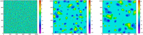Potential vorticity is represented using 80 contour levels, and the simulation is initialised with the spatially random smooth PV field shown in figure 1, left, which has spectrum (11) $\mathcal{C}\left(k\right)=c(k_d^2+k^2)k^{2p-3}\exp [-(p-1)(k/k_0{)}^2].$(11) Here $\mathcal{C}\left(k\right)$ is the power spectrum of $C\equiv ⟨q^2⟩/2$, p = 3, and the spectral peak wavenumber is set to $k_0=40$, so that the characteristic length scale of the initial PV field is the deformation length $L_D=1/40$. The constant c is chosen so that $|q{|}_{\mathrm{m}\mathrm{a}\mathrm{x}}=4\pi$.

Figure 1. Potential vorticity field at t = 0 (left), t = 20, 000 (middle) and t = 50, 200 (right). (Colour online).

3.2. Flow structure and emergence of fronts

The PV field quickly develops mixed regions, which increase in characteristic size as the flow evolves, and on which PV is roughly homogenised. These mixed regions are bounded by PV fronts, narrow bands of width $\mathrm{O}\left(L_D\right)$, over which the PV gradients are steep and the PV transitions from its value on one mixed level to the next. Well-developed mixed regions are visible already at t = 20, 000, for example in the positive (green–yellow) and negative (blue) multilevel vortices at $(100,600)$ in the middle panel of figure 1. The PV fronts are visible as sharp transitions between the lower mixed level (light green) and upper mixed level (yellow), and similarly for the negative vortex. By t = 50, 200 (figure 1, right) the mixed regions have grown larger, the number of vortices has fallen off, and more of the vortices contain clearly defined mixed PV levels with intermediate PV fronts.

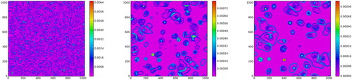
Figure 2 shows the kinetic energy density corresponding to the PV in figure 1. By t = 20, 000 (middle panel) the frontal structure has clearly emerged, as indicated by strong ribbon-like jets collocated with the fronts. At this stage the exterior fronts bounding the lowest non-zero mixed regions are particularly well-developed, while the interior fronts and their collocated jets are still weak. By t = 50, 200 both the exterior fronts and the interior fronts bounding the secondary mixed level are well-developed, as indicated by the strength of their collocated jets. This frontal structure, with two concentric fronts bounding two main mixed levels of PV, persists throughout the simulation, as it must due to PV conservation.

Figure 2. Kinetic energy density at t = 0 (left), t = 20, 000 (middle) and $t=50,200$ (right). (Colour online).

At later times the mixed PV levels have grown even more distinct and much larger in size, and their bounding jets are stronger, as can be seen in figure 3, which shows the PV (left) and kinetic energy density (right) at t = 403, 000 . The two primary mixed levels at positive and negative PV values correspond to the light and dark blue regions (negative PV) and the green and yellow regions (positive PV) in the left panel. The PV fronts bounding the lower and upper mixed regions are referred to as external fronts and internal fronts, because the secondary/upper mixed level is enclosed by the lower mixed level.

Figure 3. Potential vorticity field (left) and kinetic energy density at $t=403,000$ (right). (Colour online).

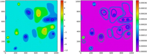
There are also many relatively small quasi-circular or weakly elliptical patches of PV with strong central peaks. These regions are referred to as “vortex cores”. Some cores, such as the patches at the lower and upper left of figure 3, left, are found outside mixed regions, and are referred to as free cores to distinguish them from cores found within mixed regions. The vortex cores are also visible in the kinetic energy density field, figure 3, right, as tightly bound groups of short quasi-circular jets with a central minima. These short weakly elliptical contours are closer in scale to $L_D$ than the long undulating frontal contours bounding large mixed regions.

4. Identification of mixed regions, fronts and free vortex cores

Two approaches are used to isolate contours and the areas they bound: the first method, also used in Burgess and Dritschel (2019), applies PV thresholds to the gridded PV fields to identify areas bounded by external fronts and internal fronts, and contained within free vortex cores. The second method uses both gridded fields and contour data to identify high-speed frontal and core contours of various lengths using thresholds on along-contour speed and arc length. These approaches allow both the high-speed contours that comprise PV fronts and bound free vortex cores and the areas contained within those contours to be studied, providing complementary viewpoints, and allowing the growth rates of the typical areas of mixed regions and cores to be compared with the properties of their bounding fronts. The methods used to extract the various structures are described in more detail below, starting with the extraction of mixed regions and vortex cores from gridded PV fields.

4.1. Moving threshold based on typical area $A_{typ}$

Both the PV-based area extraction described in section 4.2 and the high-speed contour extraction described in section 4.3 use a moving threshold based on a typical area $A_{\mathrm{t}\mathrm{y}\mathrm{p}}$ defined as (12) $A_{\mathrm{t}\mathrm{y}\mathrm{p}}\equiv \frac{\sum _{i=1}^{N\left(t\right)}{A}_i^2{\overline{q_i}}^2}{\sum _{i=1}^{N\left(t\right)}{A}_i{\overline{q_i}}^2},|q|\ge 0.25q_{\mathrm{r}\mathrm{m}\mathrm{s}}\mathrm{a}\mathrm{n}\mathrm{d}{A}_i>4\pi L_D^2.$(12) The regions i are mixed regions enclosed by high-speed frontal jets, and are identified by applying a threshold to the PV field to extract contiguous regions on which $q\ge 0.25q_{\mathrm{r}\mathrm{m}\mathrm{s}}$ and which have area $A_i>4\pi L_D^2$. This minimum area excludes tiny quasi-circular patches of PV that populate the sea of very weak PV in between the much stronger mixed regions. The area $A_i$ is the total area enclosed by front i (including the area inside the internal front, if present, and the vortex cores inside it), $\overline{q_i}$ is the PV averaged over the area $A_i$, and $N\left(t\right)$ is the total number of such regions. Note that the regions over which the sum is taken include both regions bounded by external fronts, as defined in (13(13) $q_{\mathrm{e}\mathrm{x}\mathrm{t}}=\left\{\begin{array}{l}q,\mathrm{i}\mathrm{f}|q|\ge 0.25q_{\mathrm{r}\mathrm{m}\mathrm{s}}\mathrm{a}\mathrm{n}\mathrm{d}A>A_{\mathrm{t}\mathrm{y}\mathrm{p}}/9,\\ 0,\mathrm{o}\mathrm{t}\mathrm{h}\mathrm{e}\mathrm{r}\mathrm{w}\mathrm{i}\mathrm{s}\mathrm{e},\end{array}\right.$(13) ), and free cores, as defined in equation (17(17) $q_{\mathrm{f}\mathrm{r}\mathrm{e}\mathrm{e}}=\left\{\begin{array}{l}q,\mathrm{i}\mathrm{f}|q|\ge 0.25q_{\mathrm{r}\mathrm{m}\mathrm{s}}\mathrm{a}\mathrm{n}\mathrm{d}4\pi L_D^2<A<A_{\mathrm{t}\mathrm{y}\mathrm{p}}/9,\\ 0,\mathrm{o}\mathrm{t}\mathrm{h}\mathrm{e}\mathrm{r}\mathrm{w}\mathrm{i}\mathrm{s}\mathrm{e}.\end{array}\right.$(17) ) of section 4.2 below. The inclusion of free cores in the computation of $A_{\mathrm{t}\mathrm{y}\mathrm{p}}$ distinguishes it from the typical area $A_{\mathrm{t}\mathrm{y}\mathrm{p}}^{\mathrm{e}\mathrm{x}\mathrm{t}}$ defined in (15(15) $A_{\mathrm{t}\mathrm{y}\mathrm{p}}^{\mathrm{e}\mathrm{x}\mathrm{t}}\equiv \frac{\sum _{i=1}^{N^{\mathrm{e}\mathrm{x}\mathrm{t}}\left(t\right)}{A}_i^2{\overline{q_i}}^2}{\sum _{i=1}^{N^{\mathrm{e}\mathrm{x}\mathrm{t}}\left(t\right)}{A}_i{\overline{q_i}}^2},A_i>A_{\mathrm{t}\mathrm{y}\mathrm{p}}/9,|q|\ge 0.25q_{\mathrm{r}\mathrm{m}\mathrm{s}}$(15) ) below.

The typical area $A_{\mathrm{t}\mathrm{y}\mathrm{p}}$ is shown in figure 4 (violet triangles), along with a best fit line (dashed violet), which yields $A_{\mathrm{t}\mathrm{y}\mathrm{p}}\sim t^{0.62\pm 0.03}$ over the fit interval $20,000\le t\le 660,000$ . As in Burgess and Dritschel (2019), $A_{\mathrm{t}\mathrm{y}\mathrm{p}}$ approximately follows the growth law predicted by the scaling theory in section 2: with $R_{\mathrm{t}\mathrm{y}\mathrm{p}}\sim t^{1/3}$ as in (9(9) $R\sim t^{1/3}.$(9) ), it follows that $A_{\mathrm{t}\mathrm{y}\mathrm{p}}\sim t^{2/3}$, which is approximately the case.

Figure 4. Left: typical area $A_{\mathrm{t}\mathrm{y}\mathrm{p}}^{\mathrm{e}\mathrm{x}\mathrm{t}}$ of mixed regions bounded by external fronts (black squares) with least squares best fit line (solid black), typical area $A_{\mathrm{t}\mathrm{y}\mathrm{p}}$ (violet triangles) with best fit line (dashed violet), typical area $A_{\mathrm{t}\mathrm{y}\mathrm{p}}^{\mathrm{i}\mathrm{n}\mathrm{t}}$ of mixed regions bounded by internal fronts (blue asterisks) with best fit line (dash-dot blue), and typical area $A_{\mathrm{t}\mathrm{y}\mathrm{p}}^{\mathrm{f}\mathrm{r}\mathrm{e}\mathrm{e}}$ regions within free vortex cores (magenta circles), with best fit line (magenta dotted). Right: number of mixed regions bounded by external fronts (black squares) with least squares best fit line (solid black), mixed regions bounded by internal fronts (blue asterisks) with best fit line (dash-dot blue), and regions within free vortex cores (magenta circles). (Colour online).

4.2. PV-based area extraction

To extract the areas enclosed by external and internal fronts, thresholds are applied on PV and on the area A of the enclosed region, such that (13) $q_{\mathrm{e}\mathrm{x}\mathrm{t}}=\left\{\begin{array}{l}q,\mathrm{i}\mathrm{f}|q|\ge 0.25q_{\mathrm{r}\mathrm{m}\mathrm{s}}\mathrm{a}\mathrm{n}\mathrm{d}A>A_{\mathrm{t}\mathrm{y}\mathrm{p}}/9,\\ 0,\mathrm{o}\mathrm{t}\mathrm{h}\mathrm{e}\mathrm{r}\mathrm{w}\mathrm{i}\mathrm{s}\mathrm{e},\end{array}\right.$(13) and (14) $q_{\mathrm{i}\mathrm{n}\mathrm{t}}=\left\{\begin{array}{l}q,\mathrm{i}\mathrm{f}|q|\ge 1.7q_{\mathrm{r}\mathrm{m}\mathrm{s}}\mathrm{a}\mathrm{n}\mathrm{d}A>A_{\mathrm{t}\mathrm{y}\mathrm{p}}/9,\\ 0,\mathrm{o}\mathrm{t}\mathrm{h}\mathrm{e}\mathrm{r}\mathrm{w}\mathrm{i}\mathrm{s}\mathrm{e}.\end{array}\right.$(14) Here, the subscripts ext and int indicate that the region of non-zero mixed PV is enclosed by an external front or an internal front, respectively.

The typical areas of the regions bounded by criteria (13(13) $q_{\mathrm{e}\mathrm{x}\mathrm{t}}=\left\{\begin{array}{l}q,\mathrm{i}\mathrm{f}|q|\ge 0.25q_{\mathrm{r}\mathrm{m}\mathrm{s}}\mathrm{a}\mathrm{n}\mathrm{d}A>A_{\mathrm{t}\mathrm{y}\mathrm{p}}/9,\\ 0,\mathrm{o}\mathrm{t}\mathrm{h}\mathrm{e}\mathrm{r}\mathrm{w}\mathrm{i}\mathrm{s}\mathrm{e},\end{array}\right.$(13) ) and (14(14) $q_{\mathrm{i}\mathrm{n}\mathrm{t}}=\left\{\begin{array}{l}q,\mathrm{i}\mathrm{f}|q|\ge 1.7q_{\mathrm{r}\mathrm{m}\mathrm{s}}\mathrm{a}\mathrm{n}\mathrm{d}A>A_{\mathrm{t}\mathrm{y}\mathrm{p}}/9,\\ 0,\mathrm{o}\mathrm{t}\mathrm{h}\mathrm{e}\mathrm{r}\mathrm{w}\mathrm{i}\mathrm{s}\mathrm{e}.\end{array}\right.$(14) ) are, respectively, (15) $A_{\mathrm{t}\mathrm{y}\mathrm{p}}^{\mathrm{e}\mathrm{x}\mathrm{t}}\equiv \frac{\sum _{i=1}^{N^{\mathrm{e}\mathrm{x}\mathrm{t}}\left(t\right)}{A}_i^2{\overline{q_i}}^2}{\sum _{i=1}^{N^{\mathrm{e}\mathrm{x}\mathrm{t}}\left(t\right)}{A}_i{\overline{q_i}}^2},A_i>A_{\mathrm{t}\mathrm{y}\mathrm{p}}/9,|q|\ge 0.25q_{\mathrm{r}\mathrm{m}\mathrm{s}}$(15) and (16) $A_{\mathrm{t}\mathrm{y}\mathrm{p}}^{\mathrm{i}\mathrm{n}\mathrm{t}}\equiv \frac{\sum _{i=1}^{N^{\mathrm{i}\mathrm{n}\mathrm{t}}\left(t\right)}{A}_i^2{\overline{q_i}}^2}{\sum _{i=1}^{N^{\mathrm{i}\mathrm{n}\mathrm{t}}\left(t\right)}{A}_i{\overline{q_i}}^2},A_i>A_{\mathrm{t}\mathrm{y}\mathrm{p}}/9,|q|\ge 1.7q_{\mathrm{r}\mathrm{m}\mathrm{s}},$(16) where $N^{\mathrm{e}\mathrm{x}\mathrm{t}}\left(t\right)$ and $N^{\mathrm{i}\mathrm{n}\mathrm{t}}\left(t\right)$ are the number of regions bounded by external and internal fronts, respectively. Note that $A_{\mathrm{t}\mathrm{y}\mathrm{p}}^{\mathrm{e}\mathrm{x}\mathrm{t}}$ differs from $A_{\mathrm{t}\mathrm{y}\mathrm{p}}$ in the moving lower bound $A_i>A_{\mathrm{t}\mathrm{y}\mathrm{p}}/9$ on the areas of the regions included in the sum (15(15) $A_{\mathrm{t}\mathrm{y}\mathrm{p}}^{\mathrm{e}\mathrm{x}\mathrm{t}}\equiv \frac{\sum _{i=1}^{N^{\mathrm{e}\mathrm{x}\mathrm{t}}\left(t\right)}{A}_i^2{\overline{q_i}}^2}{\sum _{i=1}^{N^{\mathrm{e}\mathrm{x}\mathrm{t}}\left(t\right)}{A}_i{\overline{q_i}}^2},A_i>A_{\mathrm{t}\mathrm{y}\mathrm{p}}/9,|q|\ge 0.25q_{\mathrm{r}\mathrm{m}\mathrm{s}}$(15) ), and $A_{\mathrm{t}\mathrm{y}\mathrm{p}}^{\mathrm{i}\mathrm{n}\mathrm{t}}$ differs from $A_{\mathrm{t}\mathrm{y}\mathrm{p}}$ in both the lower bound on area and the different PV threshold, $|q|\ge 1.7q_{\mathrm{r}\mathrm{m}\mathrm{s}}$ as opposed to $|q|\ge 0.25q_{\mathrm{r}\mathrm{m}\mathrm{s}}$.

The PV thresholds and lower bound on area A in (13(13) $q_{\mathrm{e}\mathrm{x}\mathrm{t}}=\left\{\begin{array}{l}q,\mathrm{i}\mathrm{f}|q|\ge 0.25q_{\mathrm{r}\mathrm{m}\mathrm{s}}\mathrm{a}\mathrm{n}\mathrm{d}A>A_{\mathrm{t}\mathrm{y}\mathrm{p}}/9,\\ 0,\mathrm{o}\mathrm{t}\mathrm{h}\mathrm{e}\mathrm{r}\mathrm{w}\mathrm{i}\mathrm{s}\mathrm{e},\end{array}\right.$(13) )–(14(14) $q_{\mathrm{i}\mathrm{n}\mathrm{t}}=\left\{\begin{array}{l}q,\mathrm{i}\mathrm{f}|q|\ge 1.7q_{\mathrm{r}\mathrm{m}\mathrm{s}}\mathrm{a}\mathrm{n}\mathrm{d}A>A_{\mathrm{t}\mathrm{y}\mathrm{p}}/9,\\ 0,\mathrm{o}\mathrm{t}\mathrm{h}\mathrm{e}\mathrm{r}\mathrm{w}\mathrm{i}\mathrm{s}\mathrm{e}.\end{array}\right.$(14) ) were selected by trying different values and examining the physical fields at different times to ensure that the chosen thresholds identify the correct regions. Because the values of PV on the mixed regions vary very little in time, once identified, the thresholds can be applied to the entire time integration.

The choice $A>A_{\mathrm{t}\mathrm{y}\mathrm{p}}/9$ corresponds to the threshold $L_j>L_{\mathrm{t}\mathrm{y}\mathrm{p}}/3$ on contour arclength used in section 4.3 below. Note that Burgess and Dritschel (2019) used a larger cutoff $A_{\mathrm{t}\mathrm{y}\mathrm{p}}/2$ to compute the growth rate of what here correspond to regions bounded by external fronts. Such a large threshold excludes interior fronts; taking the threshold as low as $A_{\mathrm{t}\mathrm{y}\mathrm{p}}/9$ includes interior mixed regions, while still reliably separating large mixed regions bounded by external fronts from the smaller and more slowly evolving free cores.

To extract the free vortex cores, the same PV threshold is used as for regions bounded by external fronts, but the free vortex cores must satisfy different bounds on area (17) $q_{\mathrm{f}\mathrm{r}\mathrm{e}\mathrm{e}}=\left\{\begin{array}{l}q,\mathrm{i}\mathrm{f}|q|\ge 0.25q_{\mathrm{r}\mathrm{m}\mathrm{s}}\mathrm{a}\mathrm{n}\mathrm{d}4\pi L_D^2<A<A_{\mathrm{t}\mathrm{y}\mathrm{p}}/9,\\ 0,\mathrm{o}\mathrm{t}\mathrm{h}\mathrm{e}\mathrm{r}\mathrm{w}\mathrm{i}\mathrm{s}\mathrm{e}.\end{array}\right.$(17) The upper bound $A_{\mathrm{t}\mathrm{y}\mathrm{p}}/9$ ensures that the free cores are smaller than the external and internal mixed regions. A fixed $L_D$-based upper bound was also tried, but this failed to reliably separate the free cores from dynamically active regions at times t<100, 000 , while the moving upper bound $A_{\mathrm{t}\mathrm{y}\mathrm{p}}/9$ more reliably identified undisturbed free cores at all times. At earlier times, when the population is still developing, an $L_D$-based threshold includes many disturbed regions, which have undulating boundaries, and which are undergoing merger, and therefore should not be classified as free cores. A fixed $L_D$-based threshold has the additional disadvantage that the regions selected are not guaranteed to be smaller than regions bounded by external fronts, while the thresholds (13(13) $q_{\mathrm{e}\mathrm{x}\mathrm{t}}=\left\{\begin{array}{l}q,\mathrm{i}\mathrm{f}|q|\ge 0.25q_{\mathrm{r}\mathrm{m}\mathrm{s}}\mathrm{a}\mathrm{n}\mathrm{d}A>A_{\mathrm{t}\mathrm{y}\mathrm{p}}/9,\\ 0,\mathrm{o}\mathrm{t}\mathrm{h}\mathrm{e}\mathrm{r}\mathrm{w}\mathrm{i}\mathrm{s}\mathrm{e},\end{array}\right.$(13) ) and (17(17) $q_{\mathrm{f}\mathrm{r}\mathrm{e}\mathrm{e}}=\left\{\begin{array}{l}q,\mathrm{i}\mathrm{f}|q|\ge 0.25q_{\mathrm{r}\mathrm{m}\mathrm{s}}\mathrm{a}\mathrm{n}\mathrm{d}4\pi L_D^2<A<A_{\mathrm{t}\mathrm{y}\mathrm{p}}/9,\\ 0,\mathrm{o}\mathrm{t}\mathrm{h}\mathrm{e}\mathrm{r}\mathrm{w}\mathrm{i}\mathrm{s}\mathrm{e}.\end{array}\right.$(17) ) ensure there is no overlap between these populations. The lower threshold on area $4\pi L_D^2$ ensures that tiny quasi-circular patches of PV thrown off into the zero PV “sea” as the large mixed regions interact are not included in the free core field.

The typical area of the free cores is (18) $A_{\mathrm{t}\mathrm{y}\mathrm{p}}^{\mathrm{f}\mathrm{r}\mathrm{e}\mathrm{e}}\equiv \frac{\sum _{i=1}^{N^{\mathrm{f}\mathrm{r}\mathrm{e}\mathrm{e}}\left(t\right)}{A}_i^2{\overline{q_i}}^2}{\sum _{i=1}^{N^{\mathrm{f}\mathrm{r}\mathrm{e}\mathrm{e}}\left(t\right)}{A}_i{\overline{q_i}}^2},4\pi L_D^2<A<A_{\mathrm{t}\mathrm{y}\mathrm{p}}/9,|q|\ge 0.25q_{\mathrm{r}\mathrm{m}\mathrm{s}},$(18) where $N^{\mathrm{f}\mathrm{r}\mathrm{e}\mathrm{e}}\left(t\right)$ is the number of free cores. Note that $A_{\mathrm{t}\mathrm{y}\mathrm{p}}^{\mathrm{f}\mathrm{r}\mathrm{e}\mathrm{e}}$ differs from $A_{\mathrm{t}\mathrm{y}\mathrm{p}}$ by the presence of the moving upper bound on the areas $A_i$ of the regions included in the sum.

Figure 4, left, shows the growth rates of the typical areas $A_{\mathrm{t}\mathrm{y}\mathrm{p}}^{\mathrm{e}\mathrm{x}\mathrm{t},\mathrm{i}\mathrm{n}\mathrm{t},\mathrm{f}\mathrm{r}\mathrm{e}\mathrm{e}}\left(t\right)$ of regions bounded by external fronts (black squares), regions bounded by internal fronts (blue asterisks), and regions contained within free vortex cores (magenta circles), where the computation of $A_{\mathrm{t}\mathrm{y}\mathrm{p}}^{\mathrm{e}\mathrm{x}\mathrm{t},\mathrm{i}\mathrm{n}\mathrm{t},\mathrm{f}\mathrm{r}\mathrm{e}\mathrm{e}}\left(t\right)$ is restricted to the subpopulation of regions identified by thresholds (13(13) $q_{\mathrm{e}\mathrm{x}\mathrm{t}}=\left\{\begin{array}{l}q,\mathrm{i}\mathrm{f}|q|\ge 0.25q_{\mathrm{r}\mathrm{m}\mathrm{s}}\mathrm{a}\mathrm{n}\mathrm{d}A>A_{\mathrm{t}\mathrm{y}\mathrm{p}}/9,\\ 0,\mathrm{o}\mathrm{t}\mathrm{h}\mathrm{e}\mathrm{r}\mathrm{w}\mathrm{i}\mathrm{s}\mathrm{e},\end{array}\right.$(13) ), (14(14) $q_{\mathrm{i}\mathrm{n}\mathrm{t}}=\left\{\begin{array}{l}q,\mathrm{i}\mathrm{f}|q|\ge 1.7q_{\mathrm{r}\mathrm{m}\mathrm{s}}\mathrm{a}\mathrm{n}\mathrm{d}A>A_{\mathrm{t}\mathrm{y}\mathrm{p}}/9,\\ 0,\mathrm{o}\mathrm{t}\mathrm{h}\mathrm{e}\mathrm{r}\mathrm{w}\mathrm{i}\mathrm{s}\mathrm{e}.\end{array}\right.$(14) ) and (17(17) $q_{\mathrm{f}\mathrm{r}\mathrm{e}\mathrm{e}}=\left\{\begin{array}{l}q,\mathrm{i}\mathrm{f}|q|\ge 0.25q_{\mathrm{r}\mathrm{m}\mathrm{s}}\mathrm{a}\mathrm{n}\mathrm{d}4\pi L_D^2<A<A_{\mathrm{t}\mathrm{y}\mathrm{p}}/9,\\ 0,\mathrm{o}\mathrm{t}\mathrm{h}\mathrm{e}\mathrm{r}\mathrm{w}\mathrm{i}\mathrm{s}\mathrm{e}.\end{array}\right.$(17) ), respectively. Least squares best fit lines are also shown with standard error given in the exponent. The regions bounded by external and internal fronts both approximately follow the growth law $R_{\mathrm{t}\mathrm{y}\mathrm{p}}\sim t^{1/3}$ – see (9(9) $R\sim t^{1/3}.$(9) ) – found by Burgess and Dritschel (2019), with $A_{\mathrm{t}\mathrm{y}\mathrm{p}}^{\mathrm{e}\mathrm{x}\mathrm{t}}\sim t^{0.62\pm 0.02}$ for the external fronts and $A_{\mathrm{t}\mathrm{y}\mathrm{p}}^{\mathrm{i}\mathrm{n}\mathrm{t}}\sim t^{0.67\pm 0.03}$ for the internal fronts. The typical area of the free vortex cores grows more slowly, with $A_{\mathrm{t}\mathrm{y}\mathrm{p}}^{\mathrm{f}\mathrm{r}\mathrm{e}\mathrm{e}}\sim t^{0.51\pm 0.02}$. The free cores grow more steadily before $t\approx 100,000$ . At later times, interactions become less frequent, and $A_{\mathrm{t}\mathrm{y}\mathrm{p}}^{\mathrm{f}\mathrm{r}\mathrm{e}\mathrm{e}}$ remains constant for long times.

The number of regions $N^{\mathrm{e}\mathrm{x}\mathrm{t}}\left(t\right)$ of regions enclosed by external fronts, $N^{\mathrm{i}\mathrm{n}\mathrm{t}}\left(t\right)$ of regions enclosed by internal fronts, and $N^{\mathrm{f}\mathrm{r}\mathrm{e}\mathrm{e}}\left(t\right)$ of free vortex cores are shown as functions of time in figure 4, right. The number of regions enclosed by external fronts (black squares) decays like $N^{\mathrm{e}\mathrm{x}\mathrm{t}}\sim t^{-0.66\pm 0.02}$, which is in agreement with the scaling theory of Burgess and Dritschel (2019) – see (10(10) $N\sim R^{-2}\sim t^{-2/3}.$(10) ). The number of regions enclosed by internal fronts (blue asterisks) decays more steeply, with $N^{\mathrm{i}\mathrm{n}\mathrm{t}}\sim t^{-0.81\pm 0.03}$. The number of free vortex cores $N^{\mathrm{f}\mathrm{r}\mathrm{e}\mathrm{e}}$ is roughly constant, with occasional jumps upward and downward as a free core passes or fails the moving threshold on area. It should be noted that the losses and gains of cores contribute partially to the fluctuations in the free core typical area $A_{\mathrm{t}\mathrm{y}\mathrm{p}}^{\mathrm{f}\mathrm{r}\mathrm{e}\mathrm{e}}$ seen in the left panel of figure 4. Note that the number of regions is small at late times, so the power law exponents should be taken with a grain of salt. The primary point of figure 4 is that $N^{\mathrm{f}\mathrm{r}\mathrm{e}\mathrm{e}}$ exhibits qualitatively different behaviour in time – relative constancy – as compared to $N^{\mathrm{e}\mathrm{x}\mathrm{t}}$ and $N^{\mathrm{i}\mathrm{n}\mathrm{t}}$, which show a clear decay.

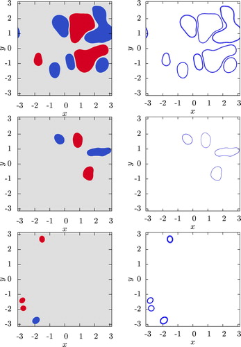
The results of applying the criteria (13(13) $q_{\mathrm{e}\mathrm{x}\mathrm{t}}=\left\{\begin{array}{l}q,\mathrm{i}\mathrm{f}|q|\ge 0.25q_{\mathrm{r}\mathrm{m}\mathrm{s}}\mathrm{a}\mathrm{n}\mathrm{d}A>A_{\mathrm{t}\mathrm{y}\mathrm{p}}/9,\\ 0,\mathrm{o}\mathrm{t}\mathrm{h}\mathrm{e}\mathrm{r}\mathrm{w}\mathrm{i}\mathrm{s}\mathrm{e},\end{array}\right.$(13) ), (14(14) $q_{\mathrm{i}\mathrm{n}\mathrm{t}}=\left\{\begin{array}{l}q,\mathrm{i}\mathrm{f}|q|\ge 1.7q_{\mathrm{r}\mathrm{m}\mathrm{s}}\mathrm{a}\mathrm{n}\mathrm{d}A>A_{\mathrm{t}\mathrm{y}\mathrm{p}}/9,\\ 0,\mathrm{o}\mathrm{t}\mathrm{h}\mathrm{e}\mathrm{r}\mathrm{w}\mathrm{i}\mathrm{s}\mathrm{e}.\end{array}\right.$(14) ) and (17(17) $q_{\mathrm{f}\mathrm{r}\mathrm{e}\mathrm{e}}=\left\{\begin{array}{l}q,\mathrm{i}\mathrm{f}|q|\ge 0.25q_{\mathrm{r}\mathrm{m}\mathrm{s}}\mathrm{a}\mathrm{n}\mathrm{d}4\pi L_D^2<A<A_{\mathrm{t}\mathrm{y}\mathrm{p}}/9,\\ 0,\mathrm{o}\mathrm{t}\mathrm{h}\mathrm{e}\mathrm{r}\mathrm{w}\mathrm{i}\mathrm{s}\mathrm{e}.\end{array}\right.$(17) ) to the PV field at $t=403,000$ are shown in the left panels of figure 5. At the top left are regions bounded by external fronts, in the middle left are regions bounded by internal fronts, and at the bottom left are free vortex cores. Positive PV is red and negative PV is blue. Comparison with the full PV field in figure 3, left, shows that the criteria (13(13) $q_{\mathrm{e}\mathrm{x}\mathrm{t}}=\left\{\begin{array}{l}q,\mathrm{i}\mathrm{f}|q|\ge 0.25q_{\mathrm{r}\mathrm{m}\mathrm{s}}\mathrm{a}\mathrm{n}\mathrm{d}A>A_{\mathrm{t}\mathrm{y}\mathrm{p}}/9,\\ 0,\mathrm{o}\mathrm{t}\mathrm{h}\mathrm{e}\mathrm{r}\mathrm{w}\mathrm{i}\mathrm{s}\mathrm{e},\end{array}\right.$(13) ), (14(14) $q_{\mathrm{i}\mathrm{n}\mathrm{t}}=\left\{\begin{array}{l}q,\mathrm{i}\mathrm{f}|q|\ge 1.7q_{\mathrm{r}\mathrm{m}\mathrm{s}}\mathrm{a}\mathrm{n}\mathrm{d}A>A_{\mathrm{t}\mathrm{y}\mathrm{p}}/9,\\ 0,\mathrm{o}\mathrm{t}\mathrm{h}\mathrm{e}\mathrm{r}\mathrm{w}\mathrm{i}\mathrm{s}\mathrm{e}.\end{array}\right.$(14) ) and (17(17) $q_{\mathrm{f}\mathrm{r}\mathrm{e}\mathrm{e}}=\left\{\begin{array}{l}q,\mathrm{i}\mathrm{f}|q|\ge 0.25q_{\mathrm{r}\mathrm{m}\mathrm{s}}\mathrm{a}\mathrm{n}\mathrm{d}4\pi L_D^2<A<A_{\mathrm{t}\mathrm{y}\mathrm{p}}/9,\\ 0,\mathrm{o}\mathrm{t}\mathrm{h}\mathrm{e}\mathrm{r}\mathrm{w}\mathrm{i}\mathrm{s}\mathrm{e}.\end{array}\right.$(17) ) extract regions bounded by external fronts, internal fronts and located within free vortex cores extremely well.

Figure 5. Results of the mixed region and free vortex core extractions (left) and high-speed contour extractions (right) at t = 403, 000. Regions bounded by external fronts, internal fronts and contained within free vortex cores are shown in the top, middle and bottom left panels, respectively, while the corresponding bounding contours composing the external PV fronts, internal PV fronts and boundaries of the free cores are shown in the top, middle and bottom right, respectively. (Colour online).

4.3. High-speed contour extraction

To complement the area extractions of mixed levels and vortex cores, high-speed PV contours making up the external and internal frontal jets and the free cores are identified using a combination of gridded fields and contour data. The high-speed frontal and core contours are visible in the kinetic energy density field shown in figure 3, right, as cyan and dark blue string-like structures.

To isolate contours belonging to external and internal fronts, masks based on the PV field were first applied to the gridded velocity field. For the external frontal jets the velocity field was set to zero except where $0.25q_{\mathrm{r}\mathrm{m}\mathrm{s}}<|q|<1.3q_{\mathrm{r}\mathrm{m}\mathrm{s}}$, (19) ${\mathit{u}}_{\mathrm{e}\mathrm{x}\mathrm{t}}=\left\{\begin{array}{l}\mathit{u},0.25q_{\mathrm{r}\mathrm{m}\mathrm{s}}<|q|<1.3q_{\mathrm{r}\mathrm{m}\mathrm{s}}\\ 0,\mathrm{o}\mathrm{t}\mathrm{h}\mathrm{e}\mathrm{r}\mathrm{w}\mathrm{i}\mathrm{s}\mathrm{e}.\end{array}\right.$(19) For the internal frontal jets the velocity field was set to zero except in regions where $1.7q_{\mathrm{r}\mathrm{m}\mathrm{s}}<|q|<2q_{\mathrm{r}\mathrm{m}\mathrm{s}}$, (20) ${\mathit{u}}_{\mathrm{i}\mathrm{n}\mathrm{t}}=\left\{\begin{array}{l}\mathit{u},1.7q_{\mathrm{r}\mathrm{m}\mathrm{s}}<|q|<2q_{\mathrm{r}\mathrm{m}\mathrm{s}}\\ 0,\mathrm{o}\mathrm{t}\mathrm{h}\mathrm{e}\mathrm{r}\mathrm{w}\mathrm{i}\mathrm{s}\mathrm{e}.\end{array}\right.$(20) These threshold values were chosen by examining the resulting kinetic energy density fields and confirming that (19(19) ${\mathit{u}}_{\mathrm{e}\mathrm{x}\mathrm{t}}=\left\{\begin{array}{l}\mathit{u},0.25q_{\mathrm{r}\mathrm{m}\mathrm{s}}<|q|<1.3q_{\mathrm{r}\mathrm{m}\mathrm{s}}\\ 0,\mathrm{o}\mathrm{t}\mathrm{h}\mathrm{e}\mathrm{r}\mathrm{w}\mathrm{i}\mathrm{s}\mathrm{e}.\end{array}\right.$(19) ) and (20(20) ${\mathit{u}}_{\mathrm{i}\mathrm{n}\mathrm{t}}=\left\{\begin{array}{l}\mathit{u},1.7q_{\mathrm{r}\mathrm{m}\mathrm{s}}<|q|<2q_{\mathrm{r}\mathrm{m}\mathrm{s}}\\ 0,\mathrm{o}\mathrm{t}\mathrm{h}\mathrm{e}\mathrm{r}\mathrm{w}\mathrm{i}\mathrm{s}\mathrm{e}.\end{array}\right.$(20) ) isolate the external fronts bounding the lowest non-zero mixed PV level and the internal fronts bounding the secondary mixed levels within each vortex, respectively.

The second step in identifying the frontal jet contours is to interpolate the masked velocity onto the contours using two-point Gaussian quadrature to compute circulation $C_j$ and arc length $L_j$ for contour j, and a mean along-contour speed $\overline{u_j}=|C_j|/L_j$. Contours for which $\overline{u_j}>u_{\mathrm{r}\mathrm{m}\mathrm{s}}/4$, where $u_{\mathrm{r}\mathrm{m}\mathrm{s}}$ is the rms speed of the unmasked velocity field, and for which $L_j>L_{\mathrm{t}\mathrm{y}\mathrm{p}}/3$ are then selected as belonging to frontal jets, where (21) $L_{\mathrm{t}\mathrm{y}\mathrm{p}}=\sqrt{4\pi A_{\mathrm{t}\mathrm{y}\mathrm{p}}},$(21) and the typical area $A_{\mathrm{t}\mathrm{y}\mathrm{p}}$ is defined in (12(12) $A_{\mathrm{t}\mathrm{y}\mathrm{p}}\equiv \frac{\sum _{i=1}^{N\left(t\right)}{A}_i^2{\overline{q_i}}^2}{\sum _{i=1}^{N\left(t\right)}{A}_i{\overline{q_i}}^2},|q|\ge 0.25q_{\mathrm{r}\mathrm{m}\mathrm{s}}\mathrm{a}\mathrm{n}\mathrm{d}{A}_i>4\pi L_D^2.$(12) ). The bound on along-contour speed, $\overline{u_j}>u_{\mathrm{r}\mathrm{m}\mathrm{s}}/4$, was chosen to include most of the frontal width, while excluding long, weak, filamented contours in the surrounding mixed PV field.

The results of the external and internal frontal contours identification procedures are shown in figure 5, top right and middle right, respectively. Comparing these frontal contours with the regions depicted to their left shows that they do in fact correspond with the boundaries of these regions, as desired. The thinner boundaries around internal mixed regions reflect the fact the the PV range used to mask the velocity field must be taken narrower to avoid including contours that are part of the cores or the external fronts.

To isolate contours bounding free vortex cores, the same PV thresholds as for the external frontal contours are used to mask the velocity field, (22) ${\mathit{u}}_{\mathrm{f}\mathrm{r}\mathrm{e}\mathrm{e}}=\left\{\begin{array}{l}\mathit{u},0.25q_{\mathrm{r}\mathrm{m}\mathrm{s}}<|q|<1.3q_{\mathrm{r}\mathrm{m}\mathrm{s}},\\ 0,\mathrm{o}\mathrm{t}\mathrm{h}\mathrm{e}\mathrm{r}\mathrm{w}\mathrm{i}\mathrm{s}\mathrm{e}.\end{array}\right.$(22) and the contour arc length $L_j$ is required to satisfy $4\pi L_D<L_j<L_{\mathrm{t}\mathrm{y}\mathrm{p}}/3$, corresponding to the bounds on area in (17(17) $q_{\mathrm{f}\mathrm{r}\mathrm{e}\mathrm{e}}=\left\{\begin{array}{l}q,\mathrm{i}\mathrm{f}|q|\ge 0.25q_{\mathrm{r}\mathrm{m}\mathrm{s}}\mathrm{a}\mathrm{n}\mathrm{d}4\pi L_D^2<A<A_{\mathrm{t}\mathrm{y}\mathrm{p}}/9,\\ 0,\mathrm{o}\mathrm{t}\mathrm{h}\mathrm{e}\mathrm{r}\mathrm{w}\mathrm{i}\mathrm{s}\mathrm{e}.\end{array}\right.$(17) ) and the definition of $L_{\mathrm{t}\mathrm{y}\mathrm{p}}$ in (21(21) $L_{\mathrm{t}\mathrm{y}\mathrm{p}}=\sqrt{4\pi A_{\mathrm{t}\mathrm{y}\mathrm{p}}},$(21) ). The lower bound on contour length corresponds to the lower bound on area in (17(17) $q_{\mathrm{f}\mathrm{r}\mathrm{e}\mathrm{e}}=\left\{\begin{array}{l}q,\mathrm{i}\mathrm{f}|q|\ge 0.25q_{\mathrm{r}\mathrm{m}\mathrm{s}}\mathrm{a}\mathrm{n}\mathrm{d}4\pi L_D^2<A<A_{\mathrm{t}\mathrm{y}\mathrm{p}}/9,\\ 0,\mathrm{o}\mathrm{t}\mathrm{h}\mathrm{e}\mathrm{r}\mathrm{w}\mathrm{i}\mathrm{s}\mathrm{e}.\end{array}\right.$(17) ), and serves to exclude tiny weak vortex rings thrown off by the mergers of the larger jets. These tiny vortex rings are much weaker than the jets bounding the mixed regions and free cores, but stronger than the filamentary kinetic energy associated with the sea of mixed PV, and pass the $\overline{u_j}>u_{\mathrm{r}\mathrm{m}\mathrm{s}}/4$ threshold. The high-speed contours-identified by (22(22) ${\mathit{u}}_{\mathrm{f}\mathrm{r}\mathrm{e}\mathrm{e}}=\left\{\begin{array}{l}\mathit{u},0.25q_{\mathrm{r}\mathrm{m}\mathrm{s}}<|q|<1.3q_{\mathrm{r}\mathrm{m}\mathrm{s}},\\ 0,\mathrm{o}\mathrm{t}\mathrm{h}\mathrm{e}\mathrm{r}\mathrm{w}\mathrm{i}\mathrm{s}\mathrm{e}.\end{array}\right.$(22) ) are shown in figure 5, bottom right: they correspond very well with the boundaries of the areas shown at left.

The types of deformations exhibited by the external and internal frontal contours should be compared with those exhibited by the free core boundaries. The former support long undulations, while the latter only weakly elliptical deformations. The requirement that the areas of the mixed regions exceed $A_{\mathrm{t}\mathrm{y}\mathrm{p}}/9$ ensures that conditions (13(13) $q_{\mathrm{e}\mathrm{x}\mathrm{t}}=\left\{\begin{array}{l}q,\mathrm{i}\mathrm{f}|q|\ge 0.25q_{\mathrm{r}\mathrm{m}\mathrm{s}}\mathrm{a}\mathrm{n}\mathrm{d}A>A_{\mathrm{t}\mathrm{y}\mathrm{p}}/9,\\ 0,\mathrm{o}\mathrm{t}\mathrm{h}\mathrm{e}\mathrm{r}\mathrm{w}\mathrm{i}\mathrm{s}\mathrm{e},\end{array}\right.$(13) ) and (14(14) $q_{\mathrm{i}\mathrm{n}\mathrm{t}}=\left\{\begin{array}{l}q,\mathrm{i}\mathrm{f}|q|\ge 1.7q_{\mathrm{r}\mathrm{m}\mathrm{s}}\mathrm{a}\mathrm{n}\mathrm{d}A>A_{\mathrm{t}\mathrm{y}\mathrm{p}}/9,\\ 0,\mathrm{o}\mathrm{t}\mathrm{h}\mathrm{e}\mathrm{r}\mathrm{w}\mathrm{i}\mathrm{s}\mathrm{e}.\end{array}\right.$(14) ) select regions with boundaries long enough to support undulations reminiscent of breathers governed by mKdV dynamics, so that the properties of these regions can be considered separately from smaller regions closer in size to the deformation scale $L_D$, i.e. the free cores. The difference in shape of the free cores indicates that their radii are too close to the deformation scale to support breather-like disturbances governed by mKdV dynamics.

Tables 1 and 2 summarise the parameters used in the extractions of the mixed regions and frontal contours, respectively. The first column of table 1 gives the mixed region type, the second column gives the PV threshold $q_{\mathrm{t}\mathrm{h}\mathrm{r}}$, which the PV on the region must exceed, $q>q_{\mathrm{t}\mathrm{h}\mathrm{r}}$, and columns three and four give the lower and upper bounds on area, $A_{\mathrm{t}\mathrm{h}\mathrm{r}}^{\mathrm{m}\mathrm{i}\mathrm{n}}<A<A_{\mathrm{t}\mathrm{h}\mathrm{r}}^{\mathrm{m}\mathrm{a}\mathrm{x}}$, where A is the area of the region.

Table 1. Thresholds for the extraction of mixed regions.

Mixed region type	$q_{\mathrm{t}\mathrm{h}\mathrm{r}}$	$A_{\mathrm{t}\mathrm{h}\mathrm{r}}^{\mathrm{m}\mathrm{i}\mathrm{n}}$	$A_{\mathrm{t}\mathrm{h}\mathrm{r}}^{\mathrm{m}\mathrm{a}\mathrm{x}}$
External	$0.25q_{\mathrm{r}\mathrm{m}\mathrm{s}}$	$A_{\mathrm{t}\mathrm{y}\mathrm{p}}/9$	–
Internal	$1.7q_{\mathrm{r}\mathrm{m}\mathrm{s}}\phantom{1}$	$A_{\mathrm{t}\mathrm{y}\mathrm{p}}/9$	–
Free core	$0.25q_{\mathrm{r}\mathrm{m}\mathrm{s}}$	$4\pi L_D^2$	$A_{\mathrm{t}\mathrm{y}\mathrm{p}}/9$

Note: The PV on the region must exceed $q_{\mathrm{t}\mathrm{h}\mathrm{r}}$, while the area of the region must be greater than $A_{\mathrm{t}\mathrm{h}\mathrm{r}}^{\mathrm{m}\mathrm{i}\mathrm{n}}$ and smaller than $A_{\mathrm{t}\mathrm{h}\mathrm{r}}^{\mathrm{m}\mathrm{a}\mathrm{x}}$.

Table 2. Thresholds for the extraction of high-speed frontal contours.

Contour type	$q_{\mathrm{t}\mathrm{h}\mathrm{r}}^{\mathrm{m}\mathrm{i}\mathrm{n}}$	$q_{\mathrm{t}\mathrm{h}\mathrm{r}}^{\mathrm{m}\mathrm{a}\mathrm{x}}$	$L_{\mathrm{t}\mathrm{h}\mathrm{r}}^{\mathrm{m}\mathrm{i}\mathrm{n}}$	$L_{\mathrm{t}\mathrm{h}\mathrm{r}}^{\mathrm{m}\mathrm{a}\mathrm{x}}$	${\overline{u}}_{\mathrm{t}\mathrm{h}\mathrm{r}}$
External	$0.25q_{\mathrm{r}\mathrm{m}\mathrm{s}}$	$1.3q_{\mathrm{r}\mathrm{m}\mathrm{s}}$	$L_{\mathrm{t}\mathrm{y}\mathrm{p}}/3$	–	$u_{\mathrm{r}\mathrm{m}\mathrm{s}}/4$
Internal	$1.7q_{\mathrm{r}\mathrm{m}\mathrm{s}}\phantom{1}$	$2q_{\mathrm{r}\mathrm{m}\mathrm{s}}\phantom{.1}$	$L_{\mathrm{t}\mathrm{y}\mathrm{p}}/3$	–	$u_{\mathrm{r}\mathrm{m}\mathrm{s}}/4$
Free core	$0.25q_{\mathrm{r}\mathrm{m}\mathrm{s}}$	$1.3q_{\mathrm{r}\mathrm{m}\mathrm{s}}$	$4\pi L_D$	$L_{\mathrm{t}\mathrm{y}\mathrm{p}}/3$	$u_{\mathrm{r}\mathrm{m}\mathrm{s}}/4$

Note: The PV on the region must exceed $q_{\mathrm{t}\mathrm{h}\mathrm{r}}^{\mathrm{m}\mathrm{i}\mathrm{n}}$ and be less than $q_{\mathrm{t}\mathrm{h}\mathrm{r}}^{\mathrm{m}\mathrm{a}\mathrm{x}}$, while the length of the contour must be greater than $L_{\mathrm{t}\mathrm{h}\mathrm{r}}^{\mathrm{m}\mathrm{i}\mathrm{n}}$ and less than $L_{\mathrm{t}\mathrm{h}\mathrm{r}}^{\mathrm{m}\mathrm{a}\mathrm{x}}$, and the average along-contour speed must exceed ${\overline{u}}_{\mathrm{t}\mathrm{h}\mathrm{r}}$.

Similarly, the first column of table 2 gives the contour type, the second column gives the PV threshold $q_{\mathrm{t}\mathrm{h}\mathrm{r}}$, which the PV on the enclosed region must exceed, $q>q_{\mathrm{t}\mathrm{h}\mathrm{r}}$, columns three and four gives the lower and upper bounds on contour length L, $L_{\mathrm{t}\mathrm{h}\mathrm{r}}^{\mathrm{m}\mathrm{i}\mathrm{n}}<L<L_{\mathrm{t}\mathrm{h}\mathrm{r}}^{\mathrm{m}\mathrm{a}\mathrm{x}}$, and column 5 gives the threshold on along-contour speed, $\overline{u}>{\overline{u}}_{\mathrm{t}\mathrm{h}\mathrm{r}}$.

5. Scaling properties of high-speed contours comprising frontal jets and vortex cores

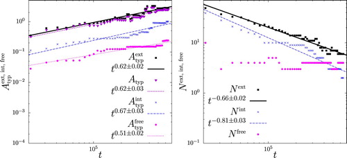
Figure 6 shows the evolution of the population total arc length $L_{\mathrm{t}\mathrm{o}\mathrm{t}}$, rms curvature ${\kappa }_{\mathrm{r}\mathrm{m}\mathrm{s}}$ and curvature fluctuation ${\kappa }_{\mathrm{f}\mathrm{l}}$ for high-speed external (left) and internal (right) frontal contours. The total arc length is computed as a sum over individual contours meeting the thresholds on speed and arc length. In the case of the external frontal contours (23) $L_{\mathrm{t}\mathrm{o}\mathrm{t}}^{\mathrm{e}\mathrm{x}\mathrm{t}}=\sum _j{L}_j,\mathrm{w}\mathrm{h}\mathrm{e}\mathrm{r}\mathrm{e}{\overline{u}}_j>u_{\mathrm{r}\mathrm{m}\mathrm{s}}/4,L_j>L_{\mathrm{t}\mathrm{y}\mathrm{p}}/3$(23) and the velocity field interpolated onto the contours to compute ${\overline{u}}_j$ has been masked as in (19(19) ${\mathit{u}}_{\mathrm{e}\mathrm{x}\mathrm{t}}=\left\{\begin{array}{l}\mathit{u},0.25q_{\mathrm{r}\mathrm{m}\mathrm{s}}<|q|<1.3q_{\mathrm{r}\mathrm{m}\mathrm{s}}\\ 0,\mathrm{o}\mathrm{t}\mathrm{h}\mathrm{e}\mathrm{r}\mathrm{w}\mathrm{i}\mathrm{s}\mathrm{e}.\end{array}\right.$(19) ). The total arc length $L_{\mathrm{t}\mathrm{o}\mathrm{t}}^{\mathrm{i}\mathrm{n}\mathrm{t}}$ for internal frontal contours is computed the same way, except with a velocity field masked as in (20(20) ${\mathit{u}}_{\mathrm{i}\mathrm{n}\mathrm{t}}=\left\{\begin{array}{l}\mathit{u},1.7q_{\mathrm{r}\mathrm{m}\mathrm{s}}<|q|<2q_{\mathrm{r}\mathrm{m}\mathrm{s}}\\ 0,\mathrm{o}\mathrm{t}\mathrm{h}\mathrm{e}\mathrm{r}\mathrm{w}\mathrm{i}\mathrm{s}\mathrm{e}.\end{array}\right.$(20) ). As shown in figure 6, left, the total arclength (open blue circle) of the external frontal contours decays as follows from (7(7) $t^{-1/3}s,t^{1/3}\kappa ,$(7) ) and (10(10) $N\sim R^{-2}\sim t^{-2/3}.$(10) ), with $L_{\mathrm{t}\mathrm{o}\mathrm{t}}^{\mathrm{e}\mathrm{x}\mathrm{t}}\sim t^{-0.32\pm 0.01}$ (solid magenta line). The total arclength of the internal frontal contours, on the other hand, decays more steeply, with $L_{\mathrm{t}\mathrm{o}\mathrm{t}}^{\mathrm{i}\mathrm{n}\mathrm{t}}\sim t^{-0.39\pm 0.02}$ (solid magenta line).

Figure 6. Total contour length $L_{\mathrm{t}\mathrm{o}\mathrm{t}}$ (open blue circles), rms curvature ${\kappa }_{\mathrm{r}\mathrm{m}\mathrm{s}}$ (open red squares), and fluctuation curvature ${\kappa }_{\mathrm{f}\mathrm{l}}$ (filled black triangles) for high-speed contours comprising external (left) and internal (right) fronts. Least squares best fit lines are also shown for ${\kappa }_{\mathrm{r}\mathrm{m}\mathrm{s}}$ (cyan), $L_{\mathrm{t}\mathrm{o}\mathrm{t}}$ (magenta) and ${\kappa }_{\mathrm{f}\mathrm{l}}$ (black). The uncertainty given is the standard error. (Colour online).

Of course, the mKdV equation conserves arclength, so decreases in total frontal length must involve processes not governed by mKdV dynamics, and which occur as a result of interactions between jets, such as reconnections and splits. These interactions generate small-scale disturbances on the jets and can induce frontal PV contours to undergo folding and form filaments that are then removed by contour surgery. Figure 7 shows an example of disturbed frontal contours undergoing filamentation at t = 141, 000 after a merger between two large mixed PV regions at t = 140, 000 . The section of jet surrounded by a rectangle is shown in close-up in the bottom panel. The innermost PV contour (blue) and the second-to-innermost contour (magenta) have folded up, forming sharp cusps, for example at $(-0.57,-0.76)$ (blue contour) and $(-0.25,-0.91)$ (magenta contour). Once two contours with the same PV value approach each other within a certain minimum distance, they are removed by contour surgery (Dritschel 1988, Dritschel and Fontane 2010), so these cusps and the associated narrow enclosed regions are expected to be removed by the numerics. The area within the blue cusps and filaments will be contributed to the mixed region, while the area within the magenta filaments will be contributed to the area between the blue and magenta contours. At the next output time (not shown) the innermost two PV contours have indeed smoothed out and the total arclength of the frontal contours has decreased. The area enclosed by the innermost two contours, which underwent filamentation, as well as the area between them, has increased. This shows that the area within the narrow extended cusps has been transferred to the mixed region and region between the two contours, as expected.

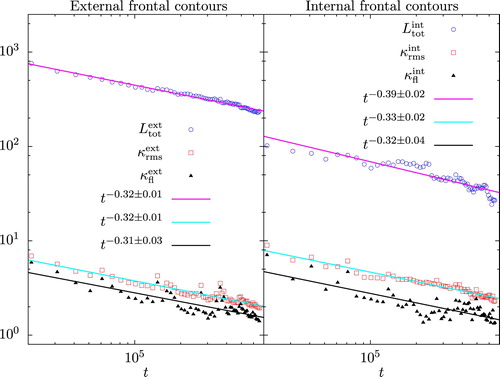
Figure 7. Disturbed PV contours undergoing filamentation after a merger at $t=140,000$. The area within the rectangle in the top panel is shown in the bottom panel: the inner two contours (blue and magenta) are undergoing filamentation. (Colour online).

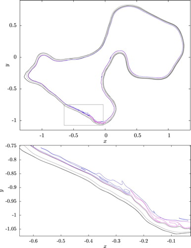
Figure 8 shows an example of a jet merger and subsequent split at a later time, and figure 9 displays the behaviour of the total contour arclength (top panel), the area enclosed by each contour (middle panel) and the area between contours (bottom panel) for the set of contours undergoing these events. Vertical lines in figure 9 indicate the reconnection and subsequent split, which coincide with cusps in the arclength. Grazing contact between the jets occurs at t = 585, 000 (figure 8, third from top left), and they merge, and then subsequently split at $t=590,000$ (figure 8, second from bottom left). Prior to the merger (top left two panels) and long after the split (bottom right two panels), the jets are relatively smooth, but after the merger they develop small-scale perturbations which persist for long times. The top panel of figure 9 shows the total arclength of the contours during these events. The arclength is relatively constant (modulo fluctuations) from t = 500, 000 to t = 580, 000 , and then shows a steady decline to a new equilibrium value as the disturbances generated by the merger and split smooth out, demonstrating how jet interactions can cause a persistent decrease in total contour length.

Figure 8. External bounding contours undergoing a reconnection and split. The time is given at the top of each panel. (Colour online).

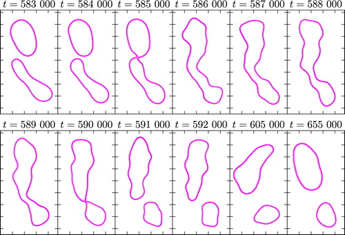
Figure 9. Total arclength (top), enclosed area (middle) and area between contours (bottom) for the contours shown in figure 8. (Colour online).

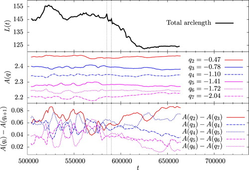
The middle panel of figure 9 shows the area enclosed by each of the contours composing the jets in figure 8, with the PV level of the contour given in the legend. The area enclosed within $q_3$ (solid blue line) decreases, while the area enclosed by its neighbouring contour $q_4$ (dash-dot blue line) increases, so that the curves move closer together. This effect is even more marked for the the contours with levels $q_5$–$q_7$, which bunch together.

The lower panel of figure 9 shows the difference $A\left(q_i\right)-A\left(q_{i+1}\right)$ of the area enclosed by adjacent contours as a function of time; $A\left(q_i\right)-A\left(q_{i+1}\right)$ is the area between the contours i and i + 1. As evident the areas between contours $q_3$ and $q_4$ decreases, as does the area between $q_5$ and $q_6$ and the area between $q_6$ and $q_7$. The area between $q_2$ and $q_3$ as well as $q_4$ and $q_5$, on the other hand, increases. This is consistent with what is observed in the flow, namely within a jet there are bands of closely spaced contours, with wider gaps in between. The changes in the area between contours start at around t = 590, 000 after the jet merger and split shown in figure 8. Hence, jet interactions such as mergers and splits are associated not only with decreases in the total arclength of the contours composing the jets, but are also responsible for sharpening the PV fronts by decreasing the area between the frontal contours.

The rms curvature for the external frontal contours is computed as (24) ${\kappa }_{\mathrm{r}\mathrm{m}\mathrm{s}}^{\mathrm{e}\mathrm{x}\mathrm{t}}=\sqrt{\frac{\sum _j\int \left[{\kappa }_j\right(s){]}^{2}s}{L_{\mathrm{t}\mathrm{o}\mathrm{t}}^{\mathrm{e}\mathrm{x}\mathrm{t}}}},$(24) where the velocity field interpolated onto the contours to compute ${\overline{u}}_j$ has been masked as in (19(19) ${\mathit{u}}_{\mathrm{e}\mathrm{x}\mathrm{t}}=\left\{\begin{array}{l}\mathit{u},0.25q_{\mathrm{r}\mathrm{m}\mathrm{s}}<|q|<1.3q_{\mathrm{r}\mathrm{m}\mathrm{s}}\\ 0,\mathrm{o}\mathrm{t}\mathrm{h}\mathrm{e}\mathrm{r}\mathrm{w}\mathrm{i}\mathrm{s}\mathrm{e}.\end{array}\right.$(19) ). The rms curvature ${\kappa }_{\mathrm{r}\mathrm{m}\mathrm{s}}^{\mathrm{i}\mathrm{n}\mathrm{t}}$ for the internal frontal contours is computed the same way, except with a velocity field masked as in (20(20) ${\mathit{u}}_{\mathrm{i}\mathrm{n}\mathrm{t}}=\left\{\begin{array}{l}\mathit{u},1.7q_{\mathrm{r}\mathrm{m}\mathrm{s}}<|q|<2q_{\mathrm{r}\mathrm{m}\mathrm{s}}\\ 0,\mathrm{o}\mathrm{t}\mathrm{h}\mathrm{e}\mathrm{r}\mathrm{w}\mathrm{i}\mathrm{s}\mathrm{e}.\end{array}\right.$(20) ). The curvature fluctuation for the external frontal contours is (25) ${\kappa }_{\mathrm{f}\mathrm{l}}^{\mathrm{e}\mathrm{x}\mathrm{t}}=\sqrt{\frac{\sum _j\int \left[{\kappa }_j\right(s)-\overline{{\kappa }_j}{]}^2\mathrm{d}s}{L_{\mathrm{t}\mathrm{o}\mathrm{t}}^{\mathrm{e}\mathrm{x}\mathrm{t}}}},\mathrm{w}\mathrm{h}\mathrm{e}\mathrm{r}\mathrm{e}{\overline{u}}_j>u_{\mathrm{r}\mathrm{m}\mathrm{s}},L_j>L_{\mathrm{t}\mathrm{y}\mathrm{p}}/3.$(25) Here $\overline{{\kappa }_j}$ is the curvature averaged over contour j, and the velocity field interpolated onto the contours to compute ${\overline{u}}_j$ has been masked as in (19(19) ${\mathit{u}}_{\mathrm{e}\mathrm{x}\mathrm{t}}=\left\{\begin{array}{l}\mathit{u},0.25q_{\mathrm{r}\mathrm{m}\mathrm{s}}<|q|<1.3q_{\mathrm{r}\mathrm{m}\mathrm{s}}\\ 0,\mathrm{o}\mathrm{t}\mathrm{h}\mathrm{e}\mathrm{r}\mathrm{w}\mathrm{i}\mathrm{s}\mathrm{e}.\end{array}\right.$(19) ). Again, the curvature fluctuation ${\kappa }_{\mathrm{f}\mathrm{l}}^{\mathrm{i}\mathrm{n}\mathrm{t}}$ for the internal frontal contours is computed the same way, except with the velocity field masked as in (20(20) ${\mathit{u}}_{\mathrm{i}\mathrm{n}\mathrm{t}}=\left\{\begin{array}{l}\mathit{u},1.7q_{\mathrm{r}\mathrm{m}\mathrm{s}}<|q|<2q_{\mathrm{r}\mathrm{m}\mathrm{s}}\\ 0,\mathrm{o}\mathrm{t}\mathrm{h}\mathrm{e}\mathrm{r}\mathrm{w}\mathrm{i}\mathrm{s}\mathrm{e}.\end{array}\right.$(20) ). The fluctuation curvature associates a meander scale with the undulating perturbations supported by the frontal contours.

As shown in figure 6, the rms curvatures for the external and internal frontal contours both decay like $t^{-1/3}$ to within the error bars, with ${\kappa }_{\mathrm{r}\mathrm{m}\mathrm{s}}^{\mathrm{e}\mathrm{x}\mathrm{t}}\sim t^{-0.32\pm 0.01}$ and ${\kappa }_{\mathrm{r}\mathrm{m}\mathrm{s}}^{\mathrm{e}\mathrm{x}\mathrm{t}}\sim t^{-0.33\pm 0.02}$, where the fit range is $20,000\le t\le 660,000$ . This is consistent with the growth rates of the typical areas $A_{\mathrm{t}\mathrm{y}\mathrm{p}}$ shown in figure 4: since the rms curvature is a measure of the typical inverse radius $1/R_{\mathrm{t}\mathrm{y}\mathrm{p}}\sim 1/\sqrt{A_{\mathrm{t}\mathrm{y}\mathrm{p}}}$, with $A_{\mathrm{t}\mathrm{y}\mathrm{p}}\sim t^{2/3}$, one would expect ${\kappa }_{\mathrm{r}\mathrm{m}\mathrm{s}}\sim t^{-1/3}$.

The fluctuation curvatures for the external and internal frontal contours also both decay approximately like $t^{-1/3}$. The fluctuation curvature associates a length scale to the undulations supported by the frontal contours, and this demonstrates that these undulations have a typical meander radius of curvature growing as $t^{1/3}$. This shows that the assumption made by Burgess and Dritschel (2019), that the wavelength of the long frontal waves – or alternatively, the meander radius of curvature in the generalisation of the scaling theory to finite-amplitude disturbances discussed in section 2 – grows like the typical mixed region radius, is a good one.

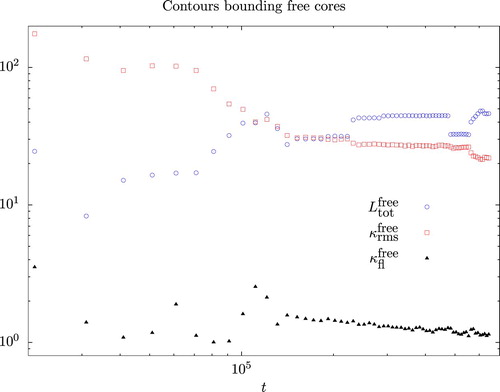
The evolution of the total arclength and curvatures for the free vortex cores is markedly different, as shown in figure 10. The total arc length $L_{\mathrm{t}\mathrm{o}\mathrm{t}}^{\mathrm{f}\mathrm{r}\mathrm{e}\mathrm{e}}$ grows irregularly and then is constant for long times at late times in the simulation, while the rms and fluctuation curvature both decay, irregularly up to $t\approx 100,000$ . Thereafter the rms curvature shows similar behaviour to the typical area of the free cores, being constant for long periods of time, and then jumping to a new value as a result of an interaction (or a region passing/failing the moving threshold). The fluctuation curvature decays more steadily than the rms curvature. The overall decay (not shown) of the squared rms curvature is $({\kappa }_{\mathrm{r}\mathrm{m}\mathrm{s}}^{\mathrm{f}\mathrm{r}\mathrm{e}\mathrm{e}}{)}^2\sim t^{-0.53\pm 0.03}$ according to a least squares fit including both early times t<100, 000 and later times. This overall decay is consistent with the growth rate of the typical area of these regions $A_{\mathrm{t}\mathrm{y}\mathrm{p}}^{\mathrm{f}\mathrm{r}\mathrm{e}\mathrm{e}}$ shown in figure 4. The behaviour of both the rms and fluctuation curvatures of the population clearly differs between early and later times, however, and the decay rates at later times are significantly smaller: on the interval $140,000\le t\le 660,000$ ${\kappa }_{\mathrm{r}\mathrm{m}\mathrm{s}}^{\mathrm{f}\mathrm{r}\mathrm{e}\mathrm{e}}\sim t^{-0.101\pm 0.008}$, while ${\kappa }_{\mathrm{f}\mathrm{l}}^{\mathrm{f}\mathrm{r}\mathrm{e}\mathrm{e}}\sim t^{-0.195\pm 0.009}$. The contours bounding the free cores, which Burgess and Dritschel (2019) excluded from their vortex census, display markedly different scaling behaviour from the contours bounding large mixed regions, justifying separate study of these regions.

Figure 10. Total contour length $L_{\mathrm{t}\mathrm{o}\mathrm{t}}$ (open blue circles), rms curvature ${\kappa }_{\mathrm{r}\mathrm{m}\mathrm{s}}$ (open red squares), and fluctuation curvature ${\kappa }_{\mathrm{f}\mathrm{l}}$ (solid black triangles) for high-speed contours bounding free vortex cores. (Colour online).

Note that though the mixed regions become large compared to the domain scale at late times, domain effects are not expected to be important to the scaling behaviour of the frontal jet curvature because the interaction length is short, with the flow speed falling off exponentially transverse to the jet (McIntyre 2008). The interactions between the jets are therefore local.

An exact general relation in fact holds between the rms curvature, the fluctuation curvature and the average arclength. The average curvature around a closed contour is given by (26) $\overline{\kappa }=\frac{1}{L}\int \kappa \mathrm{d}s=\frac{1}{L}\int \frac{\mathrm{\partial }\theta }{\mathrm{\partial }s}\mathrm{d}s=\frac{2\pi }{L},$(26) where L is the length of the contour. The exact relation (27) $\int {\kappa }^2\mathrm{d}s=\int (\kappa -\overline{\kappa }{)}^2\mathrm{d}s+\frac{4{\pi }^2}{L}$(27) follows. This relation can be generalised to an average over the population, such that (28) $\frac{1}{N_{\mathrm{c}\mathrm{o}\mathrm{n}\mathrm{t}}}\sum _j\left[\int {\kappa }_j^2\mathrm{d}s-\int ({\kappa }_j-{\overline{\kappa }}_j{)}^2\mathrm{d}s\right]=⟨\frac{4{\pi }^2}{L}⟩,$(28) where (29) $⟨\frac{1}{L}⟩=\frac{1}{N_{\mathrm{c}\mathrm{o}\mathrm{n}\mathrm{t}}}\sum _j\frac{1}{L_j}.$(29) Here, j is the contour index and $N_{\mathrm{c}\mathrm{o}\mathrm{n}\mathrm{t}}$ is the total number of contours. Figure 11 shows the left and right-hand sides of (28(28) $\frac{1}{N_{\mathrm{c}\mathrm{o}\mathrm{n}\mathrm{t}}}\sum _j\left[\int {\kappa }_j^2\mathrm{d}s-\int ({\kappa }_j-{\overline{\kappa }}_j{)}^2\mathrm{d}s\right]=⟨\frac{4{\pi }^2}{L}⟩,$(28) ), together with their ratio, $\Delta /(4{\pi }^2⟨L^{-1}⟩)$. The values of Δ and $4{\pi }^2⟨L^{-1}⟩$ are very close during the entire time interval considered, and their ratio is $\Delta /(4{\pi }^2⟨L^{-1}⟩)\approx 1$, so the relation (28(28) $\frac{1}{N_{\mathrm{c}\mathrm{o}\mathrm{n}\mathrm{t}}}\sum _j\left[\int {\kappa }_j^2\mathrm{d}s-\int ({\kappa }_j-{\overline{\kappa }}_j{)}^2\mathrm{d}s\right]=⟨\frac{4{\pi }^2}{L}⟩,$(28) ) is very close to being satisfied.

Figure 11. Check of the population-averaged relation (28(28) $\frac{1}{N_{\mathrm{c}\mathrm{o}\mathrm{n}\mathrm{t}}}\sum _j\left[\int {\kappa }_j^2\mathrm{d}s-\int ({\kappa }_j-{\overline{\kappa }}_j{)}^2\mathrm{d}s\right]=⟨\frac{4{\pi }^2}{L}⟩,$(28) ). (Colour online).

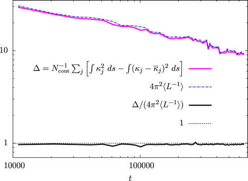
Figure 12 shows the time evolution of the average contour length of external frontal contours (top left), internal frontal contours (top right), and contours bounding free vortex cores (bottom). The average arc lengths of both the external and internal frontal contours satisfy the $t^{1/3}$ growth law, which follows from the scaling symmetries of the mKdV equation – see (6(6) $(s,t,\kappa )\mapsto (\sigma s,{\sigma }^{3}t,{\sigma }^{-1}\kappa ),$(6) ) and (7(7) $t^{-1/3}s,t^{1/3}\kappa ,$(7) ) – as shown by the least squares best fit lines (solid cyan). The fit is again over the interval $20,000\le t\le 660,000$ . The average arc length of the external contours grows more cleanly, with $L_{\mathrm{t}\mathrm{o}\mathrm{t}}^{\mathrm{e}\mathrm{x}\mathrm{t}}/N^{\mathrm{e}\mathrm{x}\mathrm{t}}\sim t^{0.33\pm 0.01}$, while $L_{\mathrm{t}\mathrm{o}\mathrm{t}}^{\mathrm{i}\mathrm{n}\mathrm{t}}/N^{\mathrm{i}\mathrm{n}\mathrm{t}}\sim t^{0.33\pm 0.02}$ shows the same extended fluctuation between $t\approx 100,000$ and $t\approx 400,000$ seen in the other internal frontal contour quantities (i.e. $A_{\mathrm{t}\mathrm{y}\mathrm{p}}^{\mathrm{i}\mathrm{n}\mathrm{t}}$ and $N^{\mathrm{i}\mathrm{n}\mathrm{t}}$ in figure 4, and, to a lesser extent, ${\kappa }_{\mathrm{r}\mathrm{m}\mathrm{s}}$ in figure 6, right).

Figure 12. Average arc length of internal frontal contours (top left), external frontal contours (top right) and contours bounding free vortex cores (bottom). Least squares best fit lines (cyan) are also shown for the internal and external frontal contours. (Colour online).

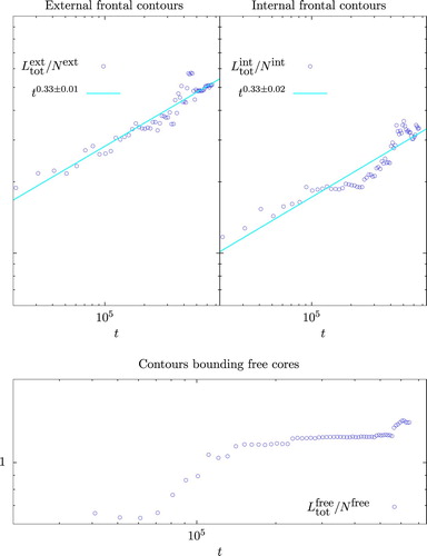
The average arclength of the contours bounding free vortex cores again displays markedly different behaviour than that of the frontal contours bounding large mixed regions. There is an upward trend, with most growth occurring between $t\approx 60,000$ and $t\approx 140,000$ , after which the average arclength grows slowly and irregularly, being constant for long stretches of time. Again, the free vortex cores clearly show distinct behaviour that justifies their separation into a distinct subpopulation in the study of the frontal contour properties.

6. Discussion and conclusions

This paper studies the scaling behaviour exhibited by the frontal jets bounding mixed regions of potential vorticity in large-scale shallow water quasigeostrophic flow at small deformation radius. Starting from a spatially random PV field with characteristic length scale $L_D$, the flow develops a complex structure with large multilevel vortices containing two main non-zero mixed levels, whose length scale L is much greater than the deformation length, $L\gg L_D$. Also present are small, weakly elliptical regions found outside the large multilevel vortices; these regions remain at approximately the same location and persist for very long times without interacting, unlike the larger vortices, which have long, undulating boundaries and drift slowly across the domain, encountering each other much more frequently.

The thin, energetic jets that bound the large mixed regions contain much of the kinetic energy and support long undulations reminiscent of breather solutions to the modified Korteweg-de Vries (mKdV) equation, which governs the path of the jet axis in the thin-jet limit (Cushman-Roisin et al. 1993, Nycander et al. 1993, Ralph and Pratt 1994). In fact, it is shown that the scaling predictions of Burgess and Dritschel (2019) for the typical radius and number of mixed PV regions alternately follow from the scaling symmetries of the mKdV equation, which also predict that the arc length of a typical front should grow like $s\sim t^{1/3}$ and the curvature decay like $\kappa \sim t^{-1/3}$. The total arc length of the external fronts bounding the lower mixed levels decays like $t^{-1/3}$, while the number of these regions falls off roughly like $t^{-2/3}$, so that the average arc length grows as $t^{1/3}$ in accord with the above prediction. The average arc length of the internal fronts bounding the upper mixed levels also grows like $t^{1/3}$. The evolution of the fronts consists of arc length preserving dynamics consistent with the mKdV equation punctuated by arc length non-conserving processes, such as filamentation of disturbed frontal contours, that occur as a result of jet reconnections and splits, which generate small-scale disturbances on the jets. The jets then lose net arc length as they smooth out. The scaling behaviour of the curvatures of the external and internal fronts bounding the lower and upper mixed levels is also consistent with mKdV scaling symmetries: the rms frontal curvature ${\kappa }_{\mathrm{r}\mathrm{m}\mathrm{s}}\sim t^{-1/3}$ and fluctuation curvature ${\kappa }_{\mathrm{f}\mathrm{l}}\sim t^{-1/3}$.

The boundaries of the free cores exhibit markedly different scaling properties than do the external and internal frontal contours bounding the large mixed regions, justifying the exclusion of the free cores from the vortex census in Burgess and Dritschel (2019). The total arc length of high-speed contours bounding free cores grows irregularly, and then is constant for long periods of time at late times in the simulation. As mentioned above, the average lengths of the external and internal frontal contours grow like $t^{1/3}$, while the average length of contours bounding free cores grows much more slowly, and is constant for long stretches at late times. While the rms and fluctuation curvatures of the external and internal contours falls off as $t^{-1/3}$, the rms and fluctuation curvatures of the contours bounding free cores decay much more slowly. The typical area of the free cores also grows more slowly than predicted by the scaling theory, with the growth rate levelling off to basically zero at late times, when the number of free cores is approximately constant, due to the rarity of their interactions. The difference in scaling properties is most likely due to size – the free cores are too close to the deformation scale to exhibit mKdV dynamics or the associated scaling symmetries. The external and internal frontal contours, on the other hand, are long enough and have a small enough rms curvature to support meanders that satisfy the thin-jet assumption and can support mKdV dynamics.

The conclusions of the present study are of course limited by the fact that only one very high resolution, long-running simulation was considered. To clarify the scaling behaviour of the internal mixed regions and their bounding fronts, and whether this behaviour actually differs in some respects from that of the external mixed regions and their frontal jets, it would be ideal to improve the statistics by considering an ensemble of similarly high resolution simulations. However, this would be a computationally intensive long-running project that is beyond the scope of the current paper. Note, for the present, that any scaling behaviour following purely from the symmetries of the mKdV equation relies only on the thin-jet approximation, and should be the same for frontal jets regardless of whether they bound internal or external mixed regions.

An interesting question that remains to be answered is the dependence of the flow structure on initial conditions, for example the characteristic scale of the initial PV field relative to the deformation radius. Another question of interest is whether thin jets and mixed regions, with associated ongoing dynamical evolution, develop even for initial conditions that are much larger scale than the deformation length. These topics are the focus of ongoing research.

Acknowledgments

The author thanks Jonas Nycander and an anonymous referee for useful comments.

Disclosure statement

No potential conflict of interest was reported by the author(s).

Additional information

Funding

This work was supported by Leverhulme Trust [ECF-2017-508].

References

- Arbic, B.K. and Flierl, G.R., Coherent vortices and kinetic energy ribbons in asymptotic, quasi two-dimensional f-plane turbulence. Phys. Fluids 2003, 15, 2177–2189. doi: 10.1063/1.1582183
- Benzi, R., Collela, M., Briscolini, M. and Santangelo, P., A simple point vortex model for two-dimensional decaying turbulence. Phys. Fluids A 1992, 4, 1036–1039. doi: 10.1063/1.858254
- Benzi, R., Paladin, G., Patarnello, S., Santangelo, P. and Vulpiani, A., Intermittency and coherent structures in two-dimensional turbulence. J. Phys. A: Math. Gen. 1986a, 19, 3771–3784. doi: 10.1088/0305-4470/19/18/023
- Benzi, R., Patarnello, S. and Santangelo, P., Self-similar coherent structures in two-dimensional decaying turbulence. J. Phys. A: Math. Gen. 1986b, 21, 1221–1237. doi: 10.1088/0305-4470/21/5/018
- Boffetta, G., De Lillo, F. and Musacchio, S., Inverse cascade in Charney-Hasegawa-Mima turbulence. Europhys. Lett. 2002, 59, 687–693. doi: 10.1209/epl/i2002-00180-y
- Burgess, B.H. and Dritschel, D.G., Long frontal waves and dynamic scaling in freely evolving equivalent barotropic flow. J. Fluid Mech. 2019, 866, R3, 347–367.
- Burgess, B.H., Dritschel, D.G. and Scott, R.K., Extended scale invariance in the vortices of freely evolving two-dimensional turbulence. Phys. Rev. Fluids 2017a, 2, 114702. doi: 10.1103/PhysRevFluids.2.114702
- Burgess, B.H., Dritschel, D.G. and Scott, R.K., Vortex scaling ranges in two-dimensional turbulence. Phys. Fluids 2017b, 29, 111104. doi: 10.1063/1.4993144
- Burgess, B.H. and Scott, R.K., Scaling theory for vortices in the two-dimensional inverse energy cascade. J. Fluid Mech. 2017, 811, 742–756. doi: 10.1017/jfm.2016.756
- Carnevale, F., McWilliams, J.C., Pomeau, Y., Weiss, J.B. and Young, W.R., Evolution of vortex statistics in two-dimensional turbulence. Phys. Rev. Lett. 1991, 66, 2735–2737. doi: 10.1103/PhysRevLett.66.2735
- Cushman-Roisin, B., Pratt, L.J. and Ralph, E.A., A general theory for equivalent barotropic thin jets. J. Phys. Oceangr. 1993, 23, 91–103. doi: 10.1175/1520-0485(1993)023<0091:AGTFEB>2.0.CO;2
- Dritschel, D.G., Contour surgery: A topological reconnection scheme for extended integrations using contour dynamics. J. Comput. Phys. 1988, 77, 240–266. doi: 10.1016/0021-9991(88)90165-9
- Dritschel, D.G. and Fontane, J., The combined Lagrangian advection method. J. Comput. Phys. 2010, 229, 5408–5417. doi: 10.1016/j.jcp.2010.03.048
- Dritschel, D.G., Scott, R.K., Macaskill, C., Gottwald, G.A. and Tran, C.V., Unifying scaling theory for vortex dynamics in two-dimensional turbulence. Phys. Rev. Lett. 2008, 101, 094501. doi: 10.1103/PhysRevLett.101.094501
- Hasegawa, A. and Mima, K., Pseudo-three-dimensional turbulence in a magnetized nonuniform plasma. Phys. Fluids 1978, 21, 87–92. doi: 10.1063/1.862083
- Huber, G. and Alstrom, P., Universal decay of vortex density in two dimensions. Phys. A 1993, 195, 448–456. doi: 10.1016/0378-4371(93)90169-5
- Iwayama, T., Fujisaka, H. and Okamoto, H., Phenomenological determination of scaling exponents in two-dimensional decaying turbulence. Prog. Theor. Phys. 1997, 98, 1219–1224. doi: 10.1143/PTP.98.1219
- Iwayama, T., Shepherd, T.G. and Watanabe, T., An “ideal” form of decaying two-dimensional turbulence. J. Fluid Mech. 2002, 456, 183–198. doi: 10.1017/S0022112001007509
- LaCasce, J.H., The vortex merger rate in freely decaying, two-dimensional turbulence. Phys. Fluids 2008, 20, 085102. doi: 10.1063/1.2957020
- Larichev, V.D. and McWilliams, J.C., Weakly decaying turbulence in an equivalent barotropic fluid. Phys. Fluids A 1991, 3, 938–950. doi: 10.1063/1.857970
- McIntyre, M.E., Potential-vorticity inversion and the wave-turbulence jigsaw: some recent clarifications. Adv. Geosci. 2008, 15, 47–56. doi: 10.5194/adgeo-15-47-2008
- McWilliams, J.C., The emergence of isolated coherent vortices in turbulent flow. J. Fluid Mech. 1984, 146, 21–43. doi: 10.1017/S0022112084001750
- McWilliams, J.C., The vortices of two-dimensional turbulence. J. Fluid Mech. 1990, 219, 361–385. doi: 10.1017/S0022112090002981
- Nycander, J., Dritschel, D.G. and Sutyrin, G.G., The dynamics of long frontal waves in the shallow-water equations. Phys. Fluids A 1993, 5, 1089–1091. doi: 10.1063/1.858592
- Pratt, L.J. and Stern, M.E., Dynamics of potential vorticity fronts and eddy detachment. J. Phys. Oceangr. 1986, 16, 1101–1120. doi: 10.1175/1520-0485(1986)016<1101:DOPVFA>2.0.CO;2
- Ralph, E.A. and Pratt, L.J., Predicting eddy detachment for an equivalent barotropic thin jet. J. Nonlinear Sci. 1994, 4, 355–374. doi: 10.1007/BF02430638
- Rhines, P. and Young, W.R., Homogenization of potential vorticity in planetary gyres. J. Fluid Mech. 1982, 122, 347–367. doi: 10.1017/S0022112082002250
- Santangelo, P., Benzi, R. and Legras, B., The generation of vortices in high-resolution, two-dimensional decaying turbulence and the influence of initial conditions on the breaking of self-similarity. Phys. Fluids A 1989, 6, 1027–1034. doi: 10.1063/1.857393
- Tran, C.V. and Dritschel, D.G., Impeded inverse energy transfer in the Charney-Hasegawa-Mima model of quasi-geostrophic flows. J. Fluid Mech. 2006, 551, 435–443. doi: 10.1017/S0022112005008384
- Watanabe, T., Dynamical scaling law in the development of drift wave turbulence. Phys. Rev. E 1997, 55, 5575–5580. doi: 10.1103/PhysRevE.55.5575
- Waugh, D.W. and Polvani, L.M., Stratospheric polar vortices. In The Stratosphere: Dynamics, Transport, and Chemistry, (Geophys. Monogr. Ser.), Vol. 190, edited by L. M. Polvani, A. H. Sobel, and D. W. Waugh, pp. 43–57, 2010 (AGU: Washington, DC).