Nonlinear wind-drift ocean currents in arctic regions

Abstract

We rely on the f-plane approximation to derive the nonlinear governing equations for arctic wind-drift flow in regions that are not in the vicinity of the North Pole. An exact solution is derived in the material (Lagrangian) framework, a setting suitable for the accurate description of the particle paths. This approach facilitates the identification of oscillations superimposed on a mean spiralling Ekman current.

Keywords:

• Wind-driven arctic current
• inertial oscillations

1. Introduction

The near-surface flow in the Arctic Ocean presents peculiar features due to the predominance of sea ice, which is currently undergoing drastic changes, shrinking in thickness and becoming more dynamic. With the surface wind as the ultimate driver of the near-surface ocean flow, sea ice is responsible for the remarkable quietness of the Arctic Ocean. While sea ice is due to the low air temperatures (averaging below $-{30}^{\circ }$C during winter and near freezing during summer) and the small solar flux (practically absent during the months of polar darkness), the low temperatures also come about because of the high reflectance or albedo (up to 80% during May) of the ocean ice cover. Plausible hypothesising that the Arctic Ocean dynamics will become more energetic if the current sea ice retreat continues (see the discussion in Mioduszweski et al. 2018) motivates in-depth studies of the way in which sea ice affects the ocean dynamics underneath it.

The classical solution to the wind-drift problem proposed more than a century ago by Ekman (1905) to explain the field observations made by Fridtjof Nansen during the 1893–1896 Arctic expedition of the Fram research vessel provides a remarkably accurate account for many commonly encountered situations (see the discussion in Morison and McPhee 2001). From a theoretical perspective, this is therefore a natural starting point from where a more complicated dynamical structure can be examined. After deriving the nonlinear governing equations for the wind-drift flow in the f-plane approximation in arctic regions outside the Amundsen Basin (where the North Pole is located, thus avoiding the singularity issue arising by the convergence of the meridians at the pole), using the material description of fluid flows, we pursue the study of an exact solution that features oscillations superimposed on an Ekman-type mean spiralling current. We also discuss how, given the capability to retrieve accurate field data about the ice motion, the mean surface current is coupled with the sea-surface stress, consisting of both air-water and ice-water stresses (partitioned depending on the sea ice concentration). We conclude with a brief discussion of the relevance of the presented approach within the wider context of more general wind-drift flows.

2. Preliminaries

Consider a Cartesian coordinate system with the zonal coordinate $x^{\prime }$ pointing eastwards, the meridional coordinate $y^{\prime }$ pointing northwards and the vertical coordinate $z^{\prime }$ pointing upwards; we use primes throughout the paper to denote physical (dimensional) variables; these will be removed when we non-dimensionalise.

The governing equations in the f-plane approximation for arctic ocean flow in the deep Canadian, Makarov and Nansen basins are (see Talley et al. 2011) the Navier-Stokes equations (1a) $\begin{array}{rl}\frac{\mathrm{D}{u}^{\prime }}{\mathrm{D}{t}^{\prime }}-f^{\prime }{v}^{\prime }& =-\frac{1}{{\rho }^{\prime }(z^{\prime })}\frac{\mathrm{\partial }{P}^{\prime }}{\mathrm{\partial }{x}^{\prime }}+{\mu }^{\prime }(\frac{{\mathrm{\partial }}^2{u}^{\prime }}{\mathrm{\partial }{x}^{\prime 2}}+\frac{{\mathrm{\partial }}^2{u}^{\prime }}{\mathrm{\partial }{y}^{\prime 2}})+{\nu }^{\prime }\frac{{\mathrm{\partial }}^2{u}^{\prime }}{\mathrm{\partial }{z}^{\prime 2}},\end{array}$(1a) (1b) $\begin{array}{rl}\frac{\mathrm{D}{v}^{\prime }}{\mathrm{D}{t}^{\prime }}+f^{\prime }{u}^{\prime }& =-\frac{1}{{\rho }^{\prime }(z^{\prime })}\frac{\mathrm{\partial }{P}^{\prime }}{\mathrm{\partial }{y}^{\prime }}+{\mu }^{\prime }(\frac{{\mathrm{\partial }}^2{v}^{\prime }}{\mathrm{\partial }{x}^{\prime 2}}+\frac{{\mathrm{\partial }}^2{v}^{\prime }}{\mathrm{\partial }{y}^{\prime 2}})+{\nu }^{\prime }\frac{{\mathrm{\partial }}^2{v}^{\prime }}{\mathrm{\partial }{z}^{\prime 2}},\end{array}$(1b) (1c) $\begin{array}{rl}\frac{\mathrm{D}{w}^{\prime }}{\mathrm{D}{t}^{\prime }}& =-\frac{1}{{\rho }^{\prime }(z^{\prime })}\frac{\mathrm{\partial }{P}^{\prime }}{\mathrm{\partial }{z}^{\prime }}-g^{\prime }+{\mu }^{\prime }(\frac{{\mathrm{\partial }}^2{w}^{\prime }}{\mathrm{\partial }{x}^{\prime 2}}+\frac{{\mathrm{\partial }}^2{w}^{\prime }}{\mathrm{\partial }{y}^{\prime 2}})+{\nu }^{\prime }\frac{{\mathrm{\partial }}^2{w}^{\prime }}{\mathrm{\partial }{z}^{\prime 2}},\end{array}$(1c) coupled with the equation of mass conservation (2) $\frac{\mathrm{D}{\rho }^{\prime }}{\mathrm{D}{t}^{\prime }}+{\rho }^{\prime }(\frac{\mathrm{\partial }{u}^{\prime }}{\mathrm{\partial }{x}^{\prime }}+\frac{\mathrm{\partial }{v}^{\prime }}{\mathrm{\partial }{y}^{\prime }}+\frac{\mathrm{\partial }{w}^{\prime }}{\mathrm{\partial }{z}^{\prime }})=0,$(2) where $t^{\prime }$ is time, $(u^{\prime },v^{\prime },w^{\prime })$ is the velocity vector, $P^{\prime }$ is the pressure, $g^{\prime }\approx 9.8\mathrm{m}{\mathrm{s}}^{-2}$ is the constant gravitational acceleration at the Earth's surface, ${\rho }^{\prime }$ is the depth-dependent water density, $f^{\prime }=2{\Omega }^{\prime }$ is the Coriolis parameter (with ${\Omega }^{\prime }\approx 7.29\times {10}^{-5}\mathrm{rad}{\mathrm{s}}^{-1}$ the constant rate of rotation of Earth about its polar axis), ${\mu }^{\prime }$ and ${\nu }^{\prime }$ are the constant horizontal and vertical eddy viscosity coefficients, respectively, and $\frac{\mathrm{D}}{\mathrm{D}{t}^{\prime }}=\frac{\mathrm{\partial }}{\mathrm{\partial }{t}^{\prime }}+u^{\prime }\frac{\mathrm{\partial }}{\mathrm{\partial }{x}^{\prime }}+v^{\prime }\frac{\mathrm{\partial }}{\mathrm{\partial }{y}^{\prime }}+w^{\prime }\frac{\mathrm{\partial }}{\mathrm{\partial }{z}^{\prime }}$ is the material derivative.

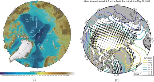
Note that the Arctic Ocean is semi-enclosed, being connected to the Atlantic Ocean somewhat narrowly on both sides of Greenland and to the Pacific Ocean through the shallow and narrow Bering Strait. The Arctic Ocean has very broad continental shelves (of 50–100 m depth, occupying more than half of the total area) surrounding a deep central region consisting of four abyssal plains (with depths close to 4 km) separated by submarine ridges (see figure 1):

• the relatively straight Lomonosov Ridge, which extends from Greenland past the North Pole to Siberia (70–200 km wide at its base lying over 4 km deep and with a narrow summit about 5–25 km wide, at depths of about 1000–1400 m), divides it into the Eurasian and Amerasian Basin;

• the relatively straight Gakkel Ridge (somewhat narrower than the Lomonosov Ridge and ranging from about 3 to 5 km depth, over 1800 km) subdivides the Eurasian Basin into the Amundsen and Nansen Basins;

• the arcuate Alpha-Mendeleev Ridge (250–1000 km wide and about 1800 km long, rising 1200 m above the surrounding ocean floor, about 3 km deep) subdivides the Amerasian Basin into the Canada and Makarov Basins.

Figure 1. The area poleward of 85${}^{\circ }$N is perennially covered with ice, with the overall sea ice extent rather asymmetric and varying annually, its minimum (in September) being in excess of 40% of the total ocean area. Apart from coastal regions, where sea ice is attached to the shoreline, the sea ice is typically in motion, the mean annual large-scale drift consisting of two primary features: the Beaufort Gyre – a clockwise (anticyclonic) motion centred at about 80${}^{\circ }$N, 155${}^{\circ }$W in the Canada Basin, and the Transpolar Drift Stream, a current away from the Siberian Coast, across the North Pole and through the Fram Strait (leading to sea ice export through this deep passage to the Atlantic Ocean that starts between the Yermal Plateau and the Morris Jessup Rise). This mean pattern is due to roughly equal contributions by winds and wind-driven near-surface currents moving ultimately in the same direction as the sea ice. (a) Bathymetry of the Arctic Ocean: broad continental shelves surround a deeper region, split down the middle by the Lomonosov Ridge (Image credit: NOAA, Colour online) and (b) Mean ice drift and sea level atmospheric pressure (Image credit: Meteorologisk Institutt and NCEP).

The most extensive basin is the Canada Basin, while the Nansen Basin is the smallest (but still about 400 km wide and over 1800 km long). By avoiding the Amundsen Basin, where the North Pole is located, the issue of convergence of meridians at the pole is not relevant in our setting. We also point out that in arctic regions the ocean temperature maximum (below 1${}^{\circ }$C, with the surface temperature roughly 1${}^{\circ }$C lower than the abyssal minimum of $-{0.5}^{\circ }$C) is at about 100–200 m depth, the density increase with depth being mainly salinity-induced and with a rather weak dependence on temperature.

Let us now describe the boundary conditions associated to wind-drift solutions to (1a(1a) $\begin{array}{rl}\frac{\mathrm{D}{u}^{\prime }}{\mathrm{D}{t}^{\prime }}-f^{\prime }{v}^{\prime }& =-\frac{1}{{\rho }^{\prime }(z^{\prime })}\frac{\mathrm{\partial }{P}^{\prime }}{\mathrm{\partial }{x}^{\prime }}+{\mu }^{\prime }(\frac{{\mathrm{\partial }}^2{u}^{\prime }}{\mathrm{\partial }{x}^{\prime 2}}+\frac{{\mathrm{\partial }}^2{u}^{\prime }}{\mathrm{\partial }{y}^{\prime 2}})+{\nu }^{\prime }\frac{{\mathrm{\partial }}^2{u}^{\prime }}{\mathrm{\partial }{z}^{\prime 2}},\end{array}$(1a) )–(2(2) $\frac{\mathrm{D}{\rho }^{\prime }}{\mathrm{D}{t}^{\prime }}+{\rho }^{\prime }(\frac{\mathrm{\partial }{u}^{\prime }}{\mathrm{\partial }{x}^{\prime }}+\frac{\mathrm{\partial }{v}^{\prime }}{\mathrm{\partial }{y}^{\prime }}+\frac{\mathrm{\partial }{w}^{\prime }}{\mathrm{\partial }{z}^{\prime }})=0,$(2) ). Firstly, the wind-drift flows are insignificant beneath the low-salinity surface layer which extends down to about 200 m, and therefore the velocity field $(u^{\prime },v^{\prime },w^{\prime })$ should present a strong depth attenuation. On the other hand, the continuity of the stress across the interface with the air leads to the surface boundary condition (3) $({\tau }_1,{\tau }_2)={\rho }^{\prime }(0){\nu }^{\prime }(\frac{\mathrm{\partial }{u}^{\prime }}{\mathrm{\partial }{z}^{\prime }},\frac{\mathrm{\partial }{v}^{\prime }}{\mathrm{\partial }{z}^{\prime }})\mathrm{on}{z}^{\prime }=0,$(3) relating the wind-stress vector $({\tau }_1,{\tau }_2)$ with the shear stress. The sea-ice cover provides a resistive force against the motion forced by the wind, with the damping of surface waves justifying the modelling assumption of a flat free surface $z^{\prime }=0$. The wind-stress vector can be partitioned as (4) $({\tau }_1,{\tau }_2)=\alpha {\mathit{\tau }}_{ice}+(1-\alpha ){\mathit{\tau }}_{air},$(4) where α is the ice-covered surface area fraction, ${\mathit{\tau }}_{ice}$ is the ice-water stress and ${\mathit{\tau }}_{air}$ is the air-water stress. The arctic sea ice is at most a few metres thick but covers millions of km${}^2$, moving in response to winds and ocean currents (see Barry et al. 1993). The ice concentration α is typically close to the unit value in winter, decreasing markedly in summer (to 0.61 in the 1990's and further to 0.46 in the next decade); see the data in Martin et al. (2014). The air-water stress is given by (see Ma et al. 2017) (5) ${\mathit{\tau }}_{air}={\rho }_a^{\prime }{c}_a|{\mathit{U}}_{\mathit{s}}|{\mathit{U}}_{\mathit{s}},$(5) where ${\rho }_a^{\prime }\approx 1.25\mathrm{kg}{\mathrm{m}}^{-3}$ is the air density, $c_a\approx 0.00125$ is the drag coefficient and ${\mathit{U}}_{\mathit{s}}$ is the horizontal wind vector at 10 m above the surface, while the air-water stress is provided by the formula (see Yang 2018) (6) ${\mathit{\tau }}_{ice}={\rho }^{\prime }(0)c_i|{\mathit{U}}_{\mathit{i}}-\mathit{U}|({\mathit{U}}_{\mathit{i}}-\mathit{U}),$(6) where ${\rho }^{\prime }(0)\approx 1026\mathrm{kg}{\mathrm{m}}^{-3}$ is the density of the surface water, $c_i\approx 0.0055$ is the ice-water drag coefficient, $\mathit{U}$ is the surface current velocity and ${\mathit{U}}_{\mathit{i}}$ is the observed ice velocity, whose daily averages are provided by combining drifting buoy observations and satellite-based data. The moving ice speed $|{\mathit{U}}_{\mathit{i}}|$ reaches 0.2 m s${}^{-1}$, twice as fast as the typical values for the under-ice current speed $|\mathit{U}|$. Moreover, since ice motion is sometimes related to advection by near-surface currents that are not wind-generated (e.g. pathways of Pacific Waters entering the Canada Basin through the Bering Street), some of the ice drift features oppose local upper ocean circulation (see Talley et al. 2011). The surface wind speeds are not particularly strong, having seasonal average of about 5 m s${}^{-1}$ with maxima rarely in excess of 12 m s${}^{-1}$ (see the data in Liu et al. 2016), and typically increase linearly with decreasing ice concentration (see Mioduszweski et al. 2018). The diurnal variability of the surface wind (in speed and direction) is generally negligible but becomes noticeable from mid-March to May, when gradual changes occur (see the data in Stegall and Zhang 2012).

In addition to requiring a rapid decay with depth of the velocity field and the stress condition (3(4) $({\tau }_1,{\tau }_2)=\alpha {\mathit{\tau }}_{ice}+(1-\alpha ){\mathit{\tau }}_{air},$(4) ) at the flat free surface $z^{\prime }=0$, we impose on the free surface a surface pressure condition (7) $P^{\prime }=P_{atm}^{\prime }\mathrm{on}{z}^{\prime }=0,$(7) where $P_{atm}^{\prime }$ is the (constant) atmospheric pressure, and the kinematic boundary condition (8) $w^{\prime }=0\mathrm{on}{z}^{\prime }=0,$(8) ensuring that there is no flux of matter at the macroscopic scale across the free boundary.

3. The governing equations at leading order

Asymptotic expansions extract the main structure of the governing equations. In order to perform them, it is necessary to first nondimensionalize the governing equations using physical scales that are representative for specific phenomena, thus clarifying the relative sizes of the terms by introducing suitable parameters that enable the pursuit of asymptotic expansions. This way order-of-magnitude estimates for the relative significance of various factors becomes mathematically possible. By reverting to dimensional variables one can then gain insight into the main physical processes at play. To implement this approach to arctic wind-drift currents, we specify the relevant physical scales (9) $\begin{array}{rll}{H}^{\prime }\approx & 50\mathrm{m}& \text{(mean depth of the arctic sub-surface layer)},\\ L^{\prime }\approx & 10\mathrm{km}& \text{(horizontal length scale)},\\ U^{\prime }\approx & 0.1\mathrm{m}{\mathrm{s}}^{-1}& \text{(horizontal velocity scale of the ocean flow)},\\ W^{\prime }\approx & {10}^{-6}\mathrm{m}{\mathrm{s}}^{-1}& \text{(vertical velocity scale of the ocean flow)},\\ {\overline{\rho }}^{\prime }\approx & 1030\mathrm{kg}{\mathrm{m}}^{-3}& \text{(average density of the arctic ocean)};\end{array}\}$(9) see the data in Talley et al. (2011) for the density, mean depth and horizontal scales, with Viudez and Dritschel (2015) providing the ratio of the vertical and horizontal velocities (so that the vertical displacement corresponds to about 0.1 m per day, confirmed by field measurements). We now define the dimensionless variables t, x, y, z, u, v, w, ρ, and p by (10) $\begin{array}{rl}{t}^{\prime }& =(L^{\prime }/U^{\prime })t,(x^{\prime },y^{\prime })=L^{\prime }(x,y),z^{\prime }=H^{\prime }z,\\ (u^{\prime },v^{\prime })& =U^{\prime }(u,v),w^{\prime }=W^{\prime }w,\\ {\rho }^{\prime }& =\overline{{\rho }^{\prime }}\rho ,P^{\prime }=P_{atm}^{\prime }+\overline{{\rho }^{\prime }}{g}^{\prime }{H}^{\prime }{\displaystyle {\int }_z^0\rho (s)\mathrm{d}s+\overline{{\rho }^{\prime }}{U}^{\prime 2}p,}\\ {\mu }^{\prime }& =U^{\prime }{L}^{\prime }\mu ,{\nu }^{\prime }=m{\mu }^{\prime },\end{array}\}$(10) with the value $U^{\prime }{L}^{\prime }\approx {10}^3{\mathrm{m}}^2{\mathrm{s}}^{-1}$ adequate for the averaged horizontal eddy viscosity and $m\ll 1$ being a proportionality factor, the vertical eddy viscosity being several orders of magnitude smaller (see Talley et al. 2011). From (1a(1a) $\begin{array}{rl}\frac{\mathrm{D}{u}^{\prime }}{\mathrm{D}{t}^{\prime }}-f^{\prime }{v}^{\prime }& =-\frac{1}{{\rho }^{\prime }(z^{\prime })}\frac{\mathrm{\partial }{P}^{\prime }}{\mathrm{\partial }{x}^{\prime }}+{\mu }^{\prime }(\frac{{\mathrm{\partial }}^2{u}^{\prime }}{\mathrm{\partial }{x}^{\prime 2}}+\frac{{\mathrm{\partial }}^2{u}^{\prime }}{\mathrm{\partial }{y}^{\prime 2}})+{\nu }^{\prime }\frac{{\mathrm{\partial }}^2{u}^{\prime }}{\mathrm{\partial }{z}^{\prime 2}},\end{array}$(1a) ) and (2(2) $\frac{\mathrm{D}{\rho }^{\prime }}{\mathrm{D}{t}^{\prime }}+{\rho }^{\prime }(\frac{\mathrm{\partial }{u}^{\prime }}{\mathrm{\partial }{x}^{\prime }}+\frac{\mathrm{\partial }{v}^{\prime }}{\mathrm{\partial }{y}^{\prime }}+\frac{\mathrm{\partial }{w}^{\prime }}{\mathrm{\partial }{z}^{\prime }})=0,$(2) ) we obtain the components of the nondimensional Navier-Stokes equation

(11a) $\begin{array}{rl}\frac{\mathrm{\partial }u}{\mathrm{\partial }t}+u\frac{\mathrm{\partial }u}{\mathrm{\partial }x}+v\frac{\mathrm{\partial }u}{\mathrm{\partial }y}+\frac{\epsilon }{\delta }w\frac{\mathrm{\partial }u}{\mathrm{\partial }z}-fv& =-\frac{1}{\rho }\frac{\mathrm{\partial }p}{\mathrm{\partial }x}+\mu (\frac{{\mathrm{\partial }}^{2}u}{\mathrm{\partial }{x}^2}+\frac{{\mathrm{\partial }}^{2}u}{\mathrm{\partial }{y}^2})+\frac{m}{{\delta }^2}\mu \frac{{\mathrm{\partial }}^{2}u}{\mathrm{\partial }{z}^2},\end{array}$(11a) (11b) $\begin{array}{rl}\frac{\mathrm{\partial }v}{\mathrm{\partial }t}+u\frac{\mathrm{\partial }v}{\mathrm{\partial }x}+v\frac{\mathrm{\partial }v}{\mathrm{\partial }y}+\frac{\epsilon }{\delta }w\frac{\mathrm{\partial }v}{\mathrm{\partial }z}+fu& =-\frac{1}{\rho }\frac{\mathrm{\partial }p}{\mathrm{\partial }y}+\mu (\frac{{\mathrm{\partial }}^{2}v}{\mathrm{\partial }{x}^2}+\frac{{\mathrm{\partial }}^{2}v}{\mathrm{\partial }{y}^2})+\frac{m}{{\delta }^2}\mu \frac{{\mathrm{\partial }}^{2}v}{\mathrm{\partial }{z}^2},\end{array}$(11b) (11c) $\begin{array}{rl}\delta \epsilon \left({\displaystyle \frac{\mathrm{\partial }w}{\mathrm{\partial }t}+u\frac{\mathrm{\partial }w}{\mathrm{\partial }x}+v\frac{\mathrm{\partial }w}{\mathrm{\partial }y}+\frac{\epsilon }{\delta }w\frac{\mathrm{\partial }w}{\mathrm{\partial }z}}\right)& =-\frac{1}{\rho }\frac{\mathrm{\partial }p}{\mathrm{\partial }z}+\epsilon \delta \mu (\frac{{\mathrm{\partial }}^{2}w}{\mathrm{\partial }{x}^2}+\frac{{\mathrm{\partial }}^{2}w}{\mathrm{\partial }{y}^2})+\frac{m\epsilon }{\delta }\mu \frac{{\mathrm{\partial }}^{2}w}{\mathrm{\partial }{z}^2},\end{array}$(11c) and the nondimensional equation of mass conservation (12) $\frac{\mathrm{\partial }\rho }{\mathrm{\partial }t}+\frac{\mathrm{\partial }(\rho u)}{\mathrm{\partial }x}+\frac{\mathrm{\partial }(\rho v)}{\mathrm{\partial }y}+\frac{\epsilon }{\delta }\frac{\mathrm{\partial }(\rho w)}{\mathrm{\partial }z}=0,$(12) respectively, expressed in terms of two important flow-parameters: the shallowness parameter δ and the ratio ε between the vertical and horizontal velocity scales, given by (13) $\delta =H^{\prime }/L^{\prime }\mathrm{and}\epsilon =W^{\prime }/U^{\prime },$(13) and where we denoted (14) $f=2{\Omega }^{\prime }{L}^{\prime }/U^{\prime }\approx \mathrm{14.5.}$(14) Within the wind-drift layer there is a balance between the viscous and the Coriolis effects. Given that $\epsilon =o(\delta )$, we infer from (11a(11a) $\begin{array}{rl}\frac{\mathrm{\partial }u}{\mathrm{\partial }t}+u\frac{\mathrm{\partial }u}{\mathrm{\partial }x}+v\frac{\mathrm{\partial }u}{\mathrm{\partial }y}+\frac{\epsilon }{\delta }w\frac{\mathrm{\partial }u}{\mathrm{\partial }z}-fv& =-\frac{1}{\rho }\frac{\mathrm{\partial }p}{\mathrm{\partial }x}+\mu (\frac{{\mathrm{\partial }}^{2}u}{\mathrm{\partial }{x}^2}+\frac{{\mathrm{\partial }}^{2}u}{\mathrm{\partial }{y}^2})+\frac{m}{{\delta }^2}\mu \frac{{\mathrm{\partial }}^{2}u}{\mathrm{\partial }{z}^2},\end{array}$(11a) ,b) that the vertical frictional stress has an effect on the near-surface horizontal flow at leading order only in the regime $m=\mathrm{O}({\delta }^2)$. We fix the value of delta, so that setting (15) $\nu =(m/{\delta }^2)\mu$(15) amounts to the nondimensional scaling (16) ${\nu }^{\prime }=\nu U^{\prime }{H}^{\prime 2}/L^{\prime },$(16) with $U^{\prime }{H}^{\prime 2}/L^{\prime }\approx 0.025{\mathrm{m}}^2{\mathrm{s}}^{-1}$ adequate for the average vertical eddy viscosity in arctic regions (see the data in Morison and McPhee 2001). On the other hand, the equation of state of seawater, derived from the first law of thermodynamics, is determined empirically in practice (see Roquet et al. 2015), specifying in relatively shallow layers a rather intricate dependence of the density on temperature and salinity (see Talley et al. 2011). However, provided that adiabatic conditions and the conservation of salinity are verified to a high degree of approximation, the equation of state becomes the incompressibility condition (17) $\frac{\mathrm{D}{\rho }^{\prime }}{\mathrm{D}{t}^{\prime }}=0$(17) (see the discussion in Cavallini and Crisciani 2013). While the thermohaline structure of the Arctic Ocean is quite complicated, the considerable excess of arctic fresh water due to direct net precipitation and to a large amount of river runoff relative to its area (comprising nearly one tenth of the Earth's overall river discharge) forms a low-density near-surface layer that greatly suppresses the heat flux (see Meincke et al. 1997). Since the changes in salinity in the upper arctic ocean (ranging up to about 5%) are typically seasonal (see Wadhams 2002), and thus not significant over the time-scale of the order of days that we consider, we can take advantage of (17(17) $\frac{\mathrm{D}{\rho }^{\prime }}{\mathrm{D}{t}^{\prime }}=0$(17) ). The non-dimensional form $\frac{\mathrm{\partial }\rho }{\mathrm{\partial }t}+u\frac{\mathrm{\partial }\rho }{\mathrm{\partial }x}+v\frac{\mathrm{\partial }\rho }{\mathrm{\partial }y}+\frac{\epsilon }{\delta }w\frac{\mathrm{\partial }\rho }{\mathrm{\partial }z}=0$ of (17(17) $\frac{\mathrm{D}{\rho }^{\prime }}{\mathrm{D}{t}^{\prime }}=0$(17) ) simplifies (12(12) $\frac{\mathrm{\partial }\rho }{\mathrm{\partial }t}+\frac{\mathrm{\partial }(\rho u)}{\mathrm{\partial }x}+\frac{\mathrm{\partial }(\rho v)}{\mathrm{\partial }y}+\frac{\epsilon }{\delta }\frac{\mathrm{\partial }(\rho w)}{\mathrm{\partial }z}=0,$(12) ) to (18) $\frac{\mathrm{\partial }u}{\mathrm{\partial }x}+\frac{\mathrm{\partial }v}{\mathrm{\partial }y}+\frac{\epsilon }{\delta }\frac{\mathrm{\partial }w}{\mathrm{\partial }z}=0.$(18) so that in the limit $\epsilon \to 0$ we now obtain from (11(11a) $\begin{array}{rl}\frac{\mathrm{\partial }u}{\mathrm{\partial }t}+u\frac{\mathrm{\partial }u}{\mathrm{\partial }x}+v\frac{\mathrm{\partial }u}{\mathrm{\partial }y}+\frac{\epsilon }{\delta }w\frac{\mathrm{\partial }u}{\mathrm{\partial }z}-fv& =-\frac{1}{\rho }\frac{\mathrm{\partial }p}{\mathrm{\partial }x}+\mu (\frac{{\mathrm{\partial }}^{2}u}{\mathrm{\partial }{x}^2}+\frac{{\mathrm{\partial }}^{2}u}{\mathrm{\partial }{y}^2})+\frac{m}{{\delta }^2}\mu \frac{{\mathrm{\partial }}^{2}u}{\mathrm{\partial }{z}^2},\end{array}$(11a) ) and (18(18) $\frac{\mathrm{\partial }u}{\mathrm{\partial }x}+\frac{\mathrm{\partial }v}{\mathrm{\partial }y}+\frac{\epsilon }{\delta }\frac{\mathrm{\partial }w}{\mathrm{\partial }z}=0.$(18) ) the governing equations for the leading-order dynamics of wind-drift arctic flows outside the Amundsen Basin: (19a) $\begin{array}{rl}\frac{\mathrm{\partial }u}{\mathrm{\partial }t}+u\frac{\mathrm{\partial }u}{\mathrm{\partial }x}+v\frac{\mathrm{\partial }u}{\mathrm{\partial }y}-fv& =-\frac{1}{\rho }\frac{\mathrm{\partial }p}{\mathrm{\partial }x}+\mu (\frac{{\mathrm{\partial }}^{2}u}{\mathrm{\partial }{x}^2}+\frac{{\mathrm{\partial }}^{2}u}{\mathrm{\partial }{y}^2})+\nu \frac{{\mathrm{\partial }}^{2}u}{\mathrm{\partial }{z}^2},\end{array}$(19a) (19b) $\begin{array}{rl}\frac{\mathrm{\partial }v}{\mathrm{\partial }t}+u\frac{\mathrm{\partial }v}{\mathrm{\partial }x}+v\frac{\mathrm{\partial }v}{\mathrm{\partial }y}+fu& =-\frac{1}{\rho }\frac{\mathrm{\partial }p}{\mathrm{\partial }y}+\mu (\frac{{\mathrm{\partial }}^{2}v}{\mathrm{\partial }{x}^2}+\frac{{\mathrm{\partial }}^{2}v}{\mathrm{\partial }{y}^2})+\nu \frac{{\mathrm{\partial }}^{2}v}{\mathrm{\partial }{z}^2},\end{array}$(19b) (19c) $\begin{array}{rl}0& =\frac{\mathrm{\partial }p}{\mathrm{\partial }z}\end{array}$(19c) and (20) $\frac{\mathrm{\partial }u}{\mathrm{\partial }x}+\frac{\mathrm{\partial }v}{\mathrm{\partial }y}=0.$(20) Given that the vertical velocity component is neglected at leading order, (8(8) $w^{\prime }=0\mathrm{on}{z}^{\prime }=0,$(8) ) is not significant for the system (19(19a) $\begin{array}{rl}\frac{\mathrm{\partial }u}{\mathrm{\partial }t}+u\frac{\mathrm{\partial }u}{\mathrm{\partial }x}+v\frac{\mathrm{\partial }u}{\mathrm{\partial }y}-fv& =-\frac{1}{\rho }\frac{\mathrm{\partial }p}{\mathrm{\partial }x}+\mu (\frac{{\mathrm{\partial }}^{2}u}{\mathrm{\partial }{x}^2}+\frac{{\mathrm{\partial }}^{2}u}{\mathrm{\partial }{y}^2})+\nu \frac{{\mathrm{\partial }}^{2}u}{\mathrm{\partial }{z}^2},\end{array}$(19a) –20(20) $\frac{\mathrm{\partial }u}{\mathrm{\partial }x}+\frac{\mathrm{\partial }v}{\mathrm{\partial }y}=0.$(20) ): the boundary conditions associated to it being (21) $\begin{array}{rl}& \frac{\mathrm{\partial }(u^2+v^2)}{\mathrm{\partial }z}<0\mathrm{for}z<0,\end{array}$(21) (22) $\begin{array}{rl}& \alpha c_i|(u_i-u,v_i-v)|(u_i-u,v_i-v)\\ & +(1-\alpha )\frac{c_a{\rho }_a}{\rho (0)}|(u_s,v_s)|(u_s,v_s)=\delta \nu (u_z,v_z)\mathrm{on}z=0,\end{array}$(22) (23) $\begin{array}{rl}& p=0\mathrm{at}z=0,\end{array}$(23) with the constraint (21(21) $\begin{array}{rl}& \frac{\mathrm{\partial }(u^2+v^2)}{\mathrm{\partial }z}<0\mathrm{for}z<0,\end{array}$(21) ) capturing the decay with depth of wind-drift flows, while (10(10) $\begin{array}{rl}{t}^{\prime }& =(L^{\prime }/U^{\prime })t,(x^{\prime },y^{\prime })=L^{\prime }(x,y),z^{\prime }=H^{\prime }z,\\ (u^{\prime },v^{\prime })& =U^{\prime }(u,v),w^{\prime }=W^{\prime }w,\\ {\rho }^{\prime }& =\overline{{\rho }^{\prime }}\rho ,P^{\prime }=P_{atm}^{\prime }+\overline{{\rho }^{\prime }}{g}^{\prime }{H}^{\prime }{\displaystyle {\int }_z^0\rho (s)\mathrm{d}s+\overline{{\rho }^{\prime }}{U}^{\prime 2}p,}\\ {\mu }^{\prime }& =U^{\prime }{L}^{\prime }\mu ,{\nu }^{\prime }=m{\mu }^{\prime },\end{array}\}$(10) ) ensures that (23(23) $\begin{array}{rl}& p=0\mathrm{at}z=0,\end{array}$(23) ) is a re-expression of (7(7) $P^{\prime }=P_{atm}^{\prime }\mathrm{on}{z}^{\prime }=0,$(7) ). Here the nondimensional scaling of the horizontal wind vector at 10 m above the surface, of the ice velocity and of the air density are provided by $\begin{array}{rl}& {\mathit{U}}_{\mathit{s}}={\mathit{U}}^{\prime }(u_s,v_s),\\ & {\mathit{U}}_{\mathit{i}}={\mathit{U}}^{\prime }(u_i,v_i),\\ & {\rho }_a^{\prime }={\overline{\rho }}^{\prime }{\rho }_a.\end{array}$ Note that, assuming knowledge of the wind stress, (22(22) $\begin{array}{rl}& \alpha c_i|(u_i-u,v_i-v)|(u_i-u,v_i-v)\\ & +(1-\alpha )\frac{c_a{\rho }_a}{\rho (0)}|(u_s,v_s)|(u_s,v_s)=\delta \nu (u_z,v_z)\mathrm{on}z=0,\end{array}$(22) ) is, in the absence of sea-ice (that is, for $\alpha =0$), a boundary condition for the tangential derivative of the wind-drift current at the surface which, in the case of the classical Ekman spiral, easily specifies the the surface current (see Talley et al. 2011). The boundary condition (22(22) $\begin{array}{rl}& \alpha c_i|(u_i-u,v_i-v)|(u_i-u,v_i-v)\\ & +(1-\alpha )\frac{c_a{\rho }_a}{\rho (0)}|(u_s,v_s)|(u_s,v_s)=\delta \nu (u_z,v_z)\mathrm{on}z=0,\end{array}$(22) ) is, however, less straightforward in the presence of a partial or total sea-ice cover, since it relates nonlinearly the tangential derivative of the wind-drift current at the surface with the surface current, assuming knowledge of the wind stress and of the ice velocity.

Due to its simple z-dependence, the system (19(19a) $\begin{array}{rl}\frac{\mathrm{\partial }u}{\mathrm{\partial }t}+u\frac{\mathrm{\partial }u}{\mathrm{\partial }x}+v\frac{\mathrm{\partial }u}{\mathrm{\partial }y}-fv& =-\frac{1}{\rho }\frac{\mathrm{\partial }p}{\mathrm{\partial }x}+\mu (\frac{{\mathrm{\partial }}^{2}u}{\mathrm{\partial }{x}^2}+\frac{{\mathrm{\partial }}^{2}u}{\mathrm{\partial }{y}^2})+\nu \frac{{\mathrm{\partial }}^{2}u}{\mathrm{\partial }{z}^2},\end{array}$(19a) –20(20) $\frac{\mathrm{\partial }u}{\mathrm{\partial }x}+\frac{\mathrm{\partial }v}{\mathrm{\partial }y}=0.$(20) ) appears to admit solutions that consist of layered depth-dependent 2D incompressible horizontal flows. This possibility will be explored in detail in the next section.

4. Main result

Within the Lagrangian framework, we will show that an explicit solution to the governing equations for the leading-order dynamics of wind-drift arctic flows outside the Amundsen Basin, (19(19a) $\begin{array}{rl}\frac{\mathrm{\partial }u}{\mathrm{\partial }t}+u\frac{\mathrm{\partial }u}{\mathrm{\partial }x}+v\frac{\mathrm{\partial }u}{\mathrm{\partial }y}-fv& =-\frac{1}{\rho }\frac{\mathrm{\partial }p}{\mathrm{\partial }x}+\mu (\frac{{\mathrm{\partial }}^{2}u}{\mathrm{\partial }{x}^2}+\frac{{\mathrm{\partial }}^{2}u}{\mathrm{\partial }{y}^2})+\nu \frac{{\mathrm{\partial }}^{2}u}{\mathrm{\partial }{z}^2},\end{array}$(19a) –20(20) $\frac{\mathrm{\partial }u}{\mathrm{\partial }x}+\frac{\mathrm{\partial }v}{\mathrm{\partial }y}=0.$(20) ), is provided by specifying, at time t, the positions (24a) $\begin{array}{rl}x(t;a,b,z)& =a+d_1(z)t-{\displaystyle \frac{1}{k}{\mathrm{e}}^{k(b+z)}\sin [k(a-z-ct)],}\end{array}$(24a) (24b) $\begin{array}{rl}y(t;a,b,z)& =b+d_2(z)t+{\displaystyle \frac{1}{k}{\mathrm{e}}^{k(b+z)}\cos [k(a-z-ct)],}\end{array}$(24b) of the horizontally moving fluid particles in terms of the depth z, the labelling variables $(a,b)$ and the parameters k>0 and c>0, for suitably chosen functions $d_1(z)$ and $d_2(z)$. The labelling variable a runs over the entire real line, while $b\in (b_1,b_0)$ with $b_1<b_0<0$, so that $z\le 0$ ensures that the horizontal oscillations of a particle decay exponentially with increasing depth: (24(24a) $\begin{array}{rl}x(t;a,b,z)& =a+d_1(z)t-{\displaystyle \frac{1}{k}{\mathrm{e}}^{k(b+z)}\sin [k(a-z-ct)],}\end{array}$(24a) ) represents at each vertical level z beneath the ocean surface z = 0 an depth-dependent oscillatory motion (with a depth-dependent amplitude and phase shift) superimposed on a current propagating in the direction of the horizontal vector $(d_1(z),d_2(z))$.

To find the constraints on the functions $d_1(z)$ and $d_2(z)$ required for (24a(24a) $\begin{array}{rl}x(t;a,b,z)& =a+d_1(z)t-{\displaystyle \frac{1}{k}{\mathrm{e}}^{k(b+z)}\sin [k(a-z-ct)],}\end{array}$(24a) ) to represent an exact solution to the nonlinear system (19(19a) $\begin{array}{rl}\frac{\mathrm{\partial }u}{\mathrm{\partial }t}+u\frac{\mathrm{\partial }u}{\mathrm{\partial }x}+v\frac{\mathrm{\partial }u}{\mathrm{\partial }y}-fv& =-\frac{1}{\rho }\frac{\mathrm{\partial }p}{\mathrm{\partial }x}+\mu (\frac{{\mathrm{\partial }}^{2}u}{\mathrm{\partial }{x}^2}+\frac{{\mathrm{\partial }}^{2}u}{\mathrm{\partial }{y}^2})+\nu \frac{{\mathrm{\partial }}^{2}u}{\mathrm{\partial }{z}^2},\end{array}$(19a) –20(20) $\frac{\mathrm{\partial }u}{\mathrm{\partial }x}+\frac{\mathrm{\partial }v}{\mathrm{\partial }y}=0.$(20) ), we fix $z\le 0$ and set $\xi =k(a-z-ct).$ The Jacobian of the map relating at time t the particle positions to the Lagrangian labelling variables is obtained by computing the determinant $D(b,z)=1-{\mathrm{e}}^{2k(b+z)}$ of the matrix (25) $\left(\begin{array}{cc}{\displaystyle \frac{\mathrm{\partial }x}{\mathrm{\partial }a}}& {\displaystyle \frac{\mathrm{\partial }x}{\mathrm{\partial }b}}\\ {\displaystyle \frac{\mathrm{\partial }y}{\mathrm{\partial }a}}& {\displaystyle \frac{\mathrm{\partial }y}{\mathrm{\partial }b}}\end{array}\right)=\left(\begin{array}{cc}1-{\mathrm{e}}^{k(b+z)}\cos \xi & -{\mathrm{e}}^{k(b+z)}\sin \xi \\ -{\mathrm{e}}^{k(b+z)}\sin \xi & 1+{\mathrm{e}}^{k(b+z)}\cos \xi \end{array}\right)$(25) with inverse (26) $\left(\begin{array}{cc}{\displaystyle \frac{\mathrm{\partial }a}{\mathrm{\partial }x}}& {\displaystyle \frac{\mathrm{\partial }a}{\mathrm{\partial }y}}\\ {\displaystyle \frac{\mathrm{\partial }b}{\mathrm{\partial }x}}& {\displaystyle \frac{\mathrm{\partial }b}{\mathrm{\partial }y}}\end{array}\right)=\frac{1}{1-{\mathrm{e}}^{2k(b+z)}}\left(\begin{array}{cc}1+{\mathrm{e}}^{-k(b+z)}\cos \xi & {\mathrm{e}}^{-k(b+z)}\sin \xi \\ {\mathrm{e}}^{-k(b+z)}\sin \xi & 1-{\mathrm{e}}^{-k(b+z)}\cos \xi \end{array}\right).$(26) Since $D(b,z)$ is time-independent, the horizontal flow (24(24a) $\begin{array}{rl}x(t;a,b,z)& =a+d_1(z)t-{\displaystyle \frac{1}{k}{\mathrm{e}}^{k(b+z)}\sin [k(a-z-ct)],}\end{array}$(24a) ) is area-preserving and (20(20) $\frac{\mathrm{\partial }u}{\mathrm{\partial }x}+\frac{\mathrm{\partial }v}{\mathrm{\partial }y}=0.$(20) ) holds. To verify (19(19a) $\begin{array}{rl}\frac{\mathrm{\partial }u}{\mathrm{\partial }t}+u\frac{\mathrm{\partial }u}{\mathrm{\partial }x}+v\frac{\mathrm{\partial }u}{\mathrm{\partial }y}-fv& =-\frac{1}{\rho }\frac{\mathrm{\partial }p}{\mathrm{\partial }x}+\mu (\frac{{\mathrm{\partial }}^{2}u}{\mathrm{\partial }{x}^2}+\frac{{\mathrm{\partial }}^{2}u}{\mathrm{\partial }{y}^2})+\nu \frac{{\mathrm{\partial }}^{2}u}{\mathrm{\partial }{z}^2},\end{array}$(19a) ), note that the horizontal velocity of the particle (24(24a) $\begin{array}{rl}x(t;a,b,z)& =a+d_1(z)t-{\displaystyle \frac{1}{k}{\mathrm{e}}^{k(b+z)}\sin [k(a-z-ct)],}\end{array}$(24a) ) is (27a) $\begin{array}{rl}u(t;a,b,z)& ={\displaystyle \frac{\mathrm{\partial }x}{\mathrm{\partial }t}=d_1(z)+c{\mathrm{e}}^{k(b+z)}\cos [k(a-z-ct)],}\end{array}$(27a) (27b) $\begin{array}{rl}v(t;a,b,z)& ={\displaystyle \frac{\mathrm{\partial }y}{\mathrm{\partial }t}=d_2(z)+c{\mathrm{e}}^{k(b+z)}\sin [k(a-z-ct)],}\end{array}$(27b) and its acceleration is provided by means of the horizontal material derivative $\mathrm{D}/\mathrm{D}t$ as the total time-derivative of the horizontal velocity vector with components (27(27a) $\begin{array}{rl}u(t;a,b,z)& ={\displaystyle \frac{\mathrm{\partial }x}{\mathrm{\partial }t}=d_1(z)+c{\mathrm{e}}^{k(b+z)}\cos [k(a-z-ct)],}\end{array}$(27a) ), which is thus given by (28a) $\begin{array}{rl}{\displaystyle \frac{\mathrm{D}u}{\mathrm{D}t}}& ={\displaystyle \frac{\mathrm{\partial }u}{\mathrm{\partial }t}+u\frac{\mathrm{\partial }u}{\mathrm{\partial }x}+v\frac{\mathrm{\partial }u}{\mathrm{\partial }y}=k{c}^2{\mathrm{e}}^{k(b+z)}\sin [k(a-z-ct)],}\end{array}$(28a) (28b) $\begin{array}{rl}{\displaystyle \frac{\mathrm{D}v}{\mathrm{D}t}}& ={\displaystyle \frac{\mathrm{\partial }v}{\mathrm{\partial }t}+u\frac{\mathrm{\partial }v}{\mathrm{\partial }x}+v\frac{\mathrm{\partial }v}{\mathrm{\partial }y}=-k{c}^2{\mathrm{e}}^{k(b+z)}\cos [k(a-z-ct)].}\end{array}$(28b) Since $\left(\begin{array}{cc}{\displaystyle \frac{\mathrm{\partial }u}{\mathrm{\partial }x}}& {\displaystyle \frac{\mathrm{\partial }v}{\mathrm{\partial }x}}\\ {\displaystyle \frac{\mathrm{\partial }u}{\mathrm{\partial }y}}& {\displaystyle \frac{\mathrm{\partial }v}{\mathrm{\partial }y}}\end{array}\right)=\left(\begin{array}{cc}{\displaystyle \frac{\mathrm{\partial }a}{\mathrm{\partial }x}}& {\displaystyle \frac{\mathrm{\partial }b}{\mathrm{\partial }x}}\\ {\displaystyle \frac{\mathrm{\partial }a}{\mathrm{\partial }y}}& {\displaystyle \frac{\mathrm{\partial }b}{\mathrm{\partial }y}}\end{array}\right)\left(\begin{array}{cc}{\displaystyle \frac{\mathrm{\partial }u}{\mathrm{\partial }a}}& {\displaystyle \frac{\mathrm{\partial }v}{\mathrm{\partial }a}}\\ {\displaystyle \frac{\mathrm{\partial }u}{\mathrm{\partial }b}}& {\displaystyle \frac{\mathrm{\partial }v}{\mathrm{\partial }b}}\end{array}\right),$ and as (27(27a) $\begin{array}{rl}u(t;a,b,z)& ={\displaystyle \frac{\mathrm{\partial }x}{\mathrm{\partial }t}=d_1(z)+c{\mathrm{e}}^{k(b+z)}\cos [k(a-z-ct)],}\end{array}$(27a) ) yields (29) $\left(\begin{array}{cc}{\displaystyle \frac{\mathrm{\partial }u}{\mathrm{\partial }a}}& {\displaystyle \frac{\mathrm{\partial }v}{\mathrm{\partial }a}}\\ {\displaystyle \frac{\mathrm{\partial }u}{\mathrm{\partial }b}}& {\displaystyle \frac{\mathrm{\partial }v}{\mathrm{\partial }b}}\end{array}\right)=\left(\begin{array}{cc}-kc{\mathrm{e}}^{k(b+z)}\sin \xi & kc{\mathrm{e}}^{k(b+z)}\cos \xi \\ kc{\mathrm{e}}^{k(b+z)}\cos \xi & kc{\mathrm{e}}^{k(b+z)}\sin \xi \end{array}\right),$(29) together with (26(26) $\left(\begin{array}{cc}{\displaystyle \frac{\mathrm{\partial }a}{\mathrm{\partial }x}}& {\displaystyle \frac{\mathrm{\partial }a}{\mathrm{\partial }y}}\\ {\displaystyle \frac{\mathrm{\partial }b}{\mathrm{\partial }x}}& {\displaystyle \frac{\mathrm{\partial }b}{\mathrm{\partial }y}}\end{array}\right)=\frac{1}{1-{\mathrm{e}}^{2k(b+z)}}\left(\begin{array}{cc}1+{\mathrm{e}}^{-k(b+z)}\cos \xi & {\mathrm{e}}^{-k(b+z)}\sin \xi \\ {\mathrm{e}}^{-k(b+z)}\sin \xi & 1-{\mathrm{e}}^{-k(b+z)}\cos \xi \end{array}\right).$(26) ) they determine $\left(\begin{array}{cc}{\displaystyle \frac{\mathrm{\partial }u}{\mathrm{\partial }x}}& {\displaystyle \frac{\mathrm{\partial }v}{\mathrm{\partial }x}}\\ {\displaystyle \frac{\mathrm{\partial }u}{\mathrm{\partial }y}}& {\displaystyle \frac{\mathrm{\partial }v}{\mathrm{\partial }y}}\end{array}\right)=\frac{kc}{1-{\mathrm{e}}^{2k(b+z)}}\left(\begin{array}{cc}-{\mathrm{e}}^{k(b+z)}\sin \xi & {\mathrm{e}}^{k(b+z)}\cos \xi +{\mathrm{e}}^{2k(b+z)}\\ {\mathrm{e}}^{k(b+z)}\cos \xi -{\mathrm{e}}^{2k(b+z)}& {\mathrm{e}}^{k(b+z)}\sin \xi \end{array}\right),$ so that at each horizontal level the two-dimensional horizontal flow (24(24a) $\begin{array}{rl}x(t;a,b,z)& =a+d_1(z)t-{\displaystyle \frac{1}{k}{\mathrm{e}}^{k(b+z)}\sin [k(a-z-ct)],}\end{array}$(24a) ) has constant vorticity (30) $\frac{\mathrm{\partial }u}{\mathrm{\partial }y}-\frac{\mathrm{\partial }v}{\mathrm{\partial }x}=-\frac{2kc{\mathrm{e}}^{2k(b+z)}}{1-{\mathrm{e}}^{2k(b+z)}}.$(30) From (30(30) $\frac{\mathrm{\partial }u}{\mathrm{\partial }y}-\frac{\mathrm{\partial }v}{\mathrm{\partial }x}=-\frac{2kc{\mathrm{e}}^{2k(b+z)}}{1-{\mathrm{e}}^{2k(b+z)}}.$(30) ), given that (20(20) $\frac{\mathrm{\partial }u}{\mathrm{\partial }x}+\frac{\mathrm{\partial }v}{\mathrm{\partial }y}=0.$(20) ) holds, we infer that (31) $\frac{{\mathrm{\partial }}^{2}u}{\mathrm{\partial }{x}^2}+\frac{{\mathrm{\partial }}^{2}u}{\mathrm{\partial }{y}^2}=\frac{{\mathrm{\partial }}^{2}v}{\mathrm{\partial }{x}^2}+\frac{{\mathrm{\partial }}^{2}v}{\mathrm{\partial }{y}^2}=0,$(31) and using (27(27a) $\begin{array}{rl}u(t;a,b,z)& ={\displaystyle \frac{\mathrm{\partial }x}{\mathrm{\partial }t}=d_1(z)+c{\mathrm{e}}^{k(b+z)}\cos [k(a-z-ct)],}\end{array}$(27a) ), (28(28a) $\begin{array}{rl}{\displaystyle \frac{\mathrm{D}u}{\mathrm{D}t}}& ={\displaystyle \frac{\mathrm{\partial }u}{\mathrm{\partial }t}+u\frac{\mathrm{\partial }u}{\mathrm{\partial }x}+v\frac{\mathrm{\partial }u}{\mathrm{\partial }y}=k{c}^2{\mathrm{e}}^{k(b+z)}\sin [k(a-z-ct)],}\end{array}$(28a) ) and (31(31) $\frac{{\mathrm{\partial }}^{2}u}{\mathrm{\partial }{x}^2}+\frac{{\mathrm{\partial }}^{2}u}{\mathrm{\partial }{y}^2}=\frac{{\mathrm{\partial }}^{2}v}{\mathrm{\partial }{x}^2}+\frac{{\mathrm{\partial }}^{2}v}{\mathrm{\partial }{y}^2}=0,$(31) ), we can write (19(19a) $\begin{array}{rl}\frac{\mathrm{\partial }u}{\mathrm{\partial }t}+u\frac{\mathrm{\partial }u}{\mathrm{\partial }x}+v\frac{\mathrm{\partial }u}{\mathrm{\partial }y}-fv& =-\frac{1}{\rho }\frac{\mathrm{\partial }p}{\mathrm{\partial }x}+\mu (\frac{{\mathrm{\partial }}^{2}u}{\mathrm{\partial }{x}^2}+\frac{{\mathrm{\partial }}^{2}u}{\mathrm{\partial }{y}^2})+\nu \frac{{\mathrm{\partial }}^{2}u}{\mathrm{\partial }{z}^2},\end{array}$(19a) ) in the form (32a) $\begin{array}{rl}{\displaystyle \frac{\mathrm{\partial }p}{\mathrm{\partial }x}}& =\rho (z)\{\nu d_1^{″}(z)+f{d}_2(z)+(fc-k{c}^2+2\nu k^{2}c){\mathrm{e}}^{k(b+z)}\sin [k(a-z-ct)]\},\end{array}$(32a) (32b) $\begin{array}{rl}{\displaystyle \frac{\mathrm{\partial }p}{\mathrm{\partial }y}}& =\rho (z)\{\nu d_2^{″}(z)-f{d}_1(z)-(fc-k{c}^2+2\nu k^{2}c){\mathrm{e}}^{k(b+z)}\cos [k(a-z-ct)]\}.\end{array}$(32b) If (33a) $\begin{array}{rl}\nu d_1^{″}(z)+f{d}_2(z)& =0,\end{array}$(33a) (33b) $\begin{array}{rl}\nu d_2^{″}(z)-f{d}_1(z)& =0,\end{array}$(33b) then the dispersion relation (34) $c=\frac{f}{k}+2\nu k$(34) yields in view of (19(19c) $\begin{array}{rl}0& =\frac{\mathrm{\partial }p}{\mathrm{\partial }z}\end{array}$(19c) ), (23(23) $\begin{array}{rl}& p=0\mathrm{at}z=0,\end{array}$(23) ) and (32(32a) $\begin{array}{rl}{\displaystyle \frac{\mathrm{\partial }p}{\mathrm{\partial }x}}& =\rho (z)\{\nu d_1^{″}(z)+f{d}_2(z)+(fc-k{c}^2+2\nu k^{2}c){\mathrm{e}}^{k(b+z)}\sin [k(a-z-ct)]\},\end{array}$(32a) ), that the pressure perturbation p must vanish. Note that in the complex-variable notation $d(z)=d_1(z)+\mathrm{i}{d}_2(z)$ the system (33(33a) $\begin{array}{rl}\nu d_1^{″}(z)+f{d}_2(z)& =0,\end{array}$(33a) ) becomes the constant-coefficient second-order linear differential equation (35) $d^{″}(z)=\mathrm{i}\frac{f}{\nu }d(z)$(35) whose general solution is given by (36) $d(z)=A{\mathrm{e}}^{(1+\mathrm{i})\lambda z}+B{\mathrm{e}}^{-(1+\mathrm{i})\lambda z},$(36) where (37) $\lambda =\sqrt{\frac{f}{2\nu }}$(37) and $A,B\in \mathbb{C}$ are complex parameters. Since mean wind-drift currents are insignificant at great depths, the physically relevant solution is obtained by setting B = 0 in (36(36) $d(z)=A{\mathrm{e}}^{(1+\mathrm{i})\lambda z}+B{\mathrm{e}}^{-(1+\mathrm{i})\lambda z},$(36) ), in which case (36(36) $d(z)=A{\mathrm{e}}^{(1+\mathrm{i})\lambda z}+B{\mathrm{e}}^{-(1+\mathrm{i})\lambda z},$(36) ) takes the form (38) $d(z)=d(0){\mathrm{e}}^{(1+\mathrm{i})\lambda z}$(38) with $d(0)=A$ representing the mean wind-drift current at the surface z = 0. Note that the periodic functions in (24(24a) $\begin{array}{rl}x(t;a,b,z)& =a+d_1(z)t-{\displaystyle \frac{1}{k}{\mathrm{e}}^{k(b+z)}\sin [k(a-z-ct)],}\end{array}$(24a) ) have principal time-period (39) $T=\frac{2\pi }{ck},$(39) the time-average of the velocity (27(27a) $\begin{array}{rl}u(t;a,b,z)& ={\displaystyle \frac{\mathrm{\partial }x}{\mathrm{\partial }t}=d_1(z)+c{\mathrm{e}}^{k(b+z)}\cos [k(a-z-ct)],}\end{array}$(27a) ) over a period T yielding (in complex-variable notation) the mean-drift current $d(z)$, which, because of (38(38) $d(z)=d(0){\mathrm{e}}^{(1+\mathrm{i})\lambda z}$(38) ), is precisely the classical Ekman spiral (see the discussion in Talley et al. 2011). Due to the specific structure of the mean current (38(38) $d(z)=d(0){\mathrm{e}}^{(1+\mathrm{i})\lambda z}$(38) ), the rather intricate boundary condition (22(22) $\begin{array}{rl}& \alpha c_i|(u_i-u,v_i-v)|(u_i-u,v_i-v)\\ & +(1-\alpha )\frac{c_a{\rho }_a}{\rho (0)}|(u_s,v_s)|(u_s,v_s)=\delta \nu (u_z,v_z)\mathrm{on}z=0,\end{array}$(22) ) simplifies to the nonlinear vector equation

(40) $\begin{array}{rl}\alpha c_i|(u_i-{\mathfrak{d}}_1,v_i-{\mathfrak{d}}_2|(u_i-{\mathfrak{d}}_1,v_i-{\mathfrak{d}}_2)+(1-\alpha )\frac{c_a{\rho }_a}{\rho (0)}& |(u_s,v_s)|(u_s,v_s)\\ & =\delta \nu \lambda ({\mathfrak{d}}_1-{\mathfrak{d}}_2,{\mathfrak{d}}_1+{\mathfrak{d}}_2),\end{array}$(40) in which the unknown vector with components ${\mathfrak{d}}_1=d_1(0)$ and ${\mathfrak{d}}_2=d_2(0)$ represents the (nondimensional) wind-drift surface current. Subtracting the vector $\delta \nu \lambda (u_i-v_i,u_i+v_i)$ from both sides of (40(40) $\begin{array}{rl}\alpha c_i|(u_i-{\mathfrak{d}}_1,v_i-{\mathfrak{d}}_2|(u_i-{\mathfrak{d}}_1,v_i-{\mathfrak{d}}_2)+(1-\alpha )\frac{c_a{\rho }_a}{\rho (0)}& |(u_s,v_s)|(u_s,v_s)\\ & =\delta \nu \lambda ({\mathfrak{d}}_1-{\mathfrak{d}}_2,{\mathfrak{d}}_1+{\mathfrak{d}}_2),\end{array}$(40) ), after some straightforward algebraic manipulations, we can write it using the complex-variable notation $R{\mathrm{e}}^{\mathrm{i}\theta }=(u_i-{\mathfrak{d}}_1)+\mathrm{i}(v_i-{\mathfrak{d}}_2),$ equivalently in the form of the nonlinear equation (41) $R^2{\mathrm{e}}^{\mathrm{i}\theta }+\beta (1+\mathrm{i})R{\mathrm{e}}^{\mathrm{i}\theta }=Z$(41) for the unknowns $R\ge 0$ and $\theta \in [0,2\pi )$, in which $\begin{array}{rl}\beta & =\frac{\delta \nu \lambda }{\alpha c_i}>0,\\ Z& =\frac{\delta \nu \lambda }{\alpha c_i}[(u_i-v_i)+\mathrm{i}(u_i+v_i)]-\frac{(1-\alpha )c_a{\rho }_a}{\alpha c_i\rho (0)}\sqrt{u_s^2+v_s^2}(u_s+\mathrm{i}{v}_s)\in \mathbb{C},\end{array}$ are provided by field data. Note that the case Z = 0 occurs if the ice-cover is total (that is, $\alpha =1$) and the sea-ice is stationary (that is, $u_i=v_i=0$). For Z = 0 the only solution of (41(41) $R^2{\mathrm{e}}^{\mathrm{i}\theta }+\beta (1+\mathrm{i})R{\mathrm{e}}^{\mathrm{i}\theta }=Z$(41) ) is R = 0, which corresponds to $d(0)=0$: in this case there is no wind-drift current, but the wind might induce some inertial oscillations beneath the ice-cover. For $Z\ne 0$ we infer from (41(41) $R^2{\mathrm{e}}^{\mathrm{i}\theta }+\beta (1+\mathrm{i})R{\mathrm{e}}^{\mathrm{i}\theta }=Z$(41) ) that $R\ne 0$, while (42) ${\mathrm{e}}^{\mathrm{i}\theta }=\frac{Z}{R[R+\beta (1+\mathrm{i})]}.$(42) Multiplying (42(42) ${\mathrm{e}}^{\mathrm{i}\theta }=\frac{Z}{R[R+\beta (1+\mathrm{i})]}.$(42) ) with its complex-conjugate yields the quartic equation (43) $\mathcal{P}(R)=0$(43) in terms of the real polynomial $\mathcal{P}(R)=R^4+2\beta R^3+2{\beta }^2{R}^2-|Z{|}^2$. Since $\mathcal{P}(0)<0$, $\underset{R\to \pm \mathrm{\infty }}{lim}\mathcal{P}(R)=\mathrm{\infty }$ and ${\mathcal{P}}^{″}(R)=3(2R+\beta {)}^2+{\beta }^2>0$ ensures that $\mathcal{P}$ is strictly convex, there is precisely one positive root R>0 of equation (43(43) $\mathcal{P}(R)=0$(43) ), with the corresponding value of $\theta \in [0,2\pi )$ uniquely determined from (42(42) ${\mathrm{e}}^{\mathrm{i}\theta }=\frac{Z}{R[R+\beta (1+\mathrm{i})]}.$(42) ). For computational purposes, note that formulas are available for the roots of quartics (see Auckly 2007), and the fact that there is precisely one positive root singles out the formula for the physically relevant root. In any case, our analysis shows that the boundary condition (22(22) $\begin{array}{rl}& \alpha c_i|(u_i-u,v_i-v)|(u_i-u,v_i-v)\\ & +(1-\alpha )\frac{c_a{\rho }_a}{\rho (0)}|(u_s,v_s)|(u_s,v_s)=\delta \nu (u_z,v_z)\mathrm{on}z=0,\end{array}$(22) ) determines uniquely the surface current $d(0)$ from the knowledge of the surface wind and of the sea-ice velocity. While we refrain from deriving the general rather complicated formula for the deflection angle of the surface current from the direction of the surface wind, there are two cases when insight is readily available:

• If there is no sea-ice, then by setting $\alpha =0$ in (40(40) $\begin{array}{rl}\alpha c_i|(u_i-{\mathfrak{d}}_1,v_i-{\mathfrak{d}}_2|(u_i-{\mathfrak{d}}_1,v_i-{\mathfrak{d}}_2)+(1-\alpha )\frac{c_a{\rho }_a}{\rho (0)}& |(u_s,v_s)|(u_s,v_s)\\ & =\delta \nu \lambda ({\mathfrak{d}}_1-{\mathfrak{d}}_2,{\mathfrak{d}}_1+{\mathfrak{d}}_2),\end{array}$(40) ) written in complex-variable form, we infer the classical Ekman result ${\psi }_s=(\pi /4)+\psi$ between the angle ${\psi }_s$ of the surface wind and that of the surface current (with respect to the azimuthal x-axis).

• If there is no wind but a moving total ice cover (that is, $\alpha =1$ and $u_i+\mathrm{i}{v}_i=s{\mathrm{e}}^{\mathrm{i}\phi }$ with $\phi \in [0,2\pi )$ and s>0), from (40(40) $\begin{array}{rl}\alpha c_i|(u_i-{\mathfrak{d}}_1,v_i-{\mathfrak{d}}_2|(u_i-{\mathfrak{d}}_1,v_i-{\mathfrak{d}}_2)+(1-\alpha )\frac{c_a{\rho }_a}{\rho (0)}& |(u_s,v_s)|(u_s,v_s)\\ & =\delta \nu \lambda ({\mathfrak{d}}_1-{\mathfrak{d}}_2,{\mathfrak{d}}_1+{\mathfrak{d}}_2),\end{array}$(40) ) written in complex-variable form, we first infer that ${\mathfrak{d}}_1+\mathrm{i}{\mathfrak{d}}_2=r{\mathrm{e}}^{\mathrm{i}\psi }$ with r>0 and $\psi \in [0,2\pi )$. Subsequently we see that $|s{\mathrm{e}}^{\mathrm{i}\phi }-r{\mathrm{e}}^{\mathrm{i}\psi }|>0$, and therefore (40(40) $\begin{array}{rl}\alpha c_i|(u_i-{\mathfrak{d}}_1,v_i-{\mathfrak{d}}_2|(u_i-{\mathfrak{d}}_1,v_i-{\mathfrak{d}}_2)+(1-\alpha )\frac{c_a{\rho }_a}{\rho (0)}& |(u_s,v_s)|(u_s,v_s)\\ & =\delta \nu \lambda ({\mathfrak{d}}_1-{\mathfrak{d}}_2,{\mathfrak{d}}_1+{\mathfrak{d}}_2),\end{array}$(40) ) takes the form $s{\mathrm{e}}^{\mathrm{i}\phi }=r{\mathrm{e}}^{\mathrm{i}\psi }+\frac{\delta \nu \lambda }{c_i|s{\mathrm{e}}^{\mathrm{i}\phi }-r{\mathrm{e}}^{\mathrm{i}\psi }|}(1+\mathrm{i})r{\mathrm{e}}^{\mathrm{i}\psi },$ which, upon multiplying both sides with ${\mathrm{e}}^{-\mathrm{i}\psi }$, can be written as $s{\mathrm{e}}^{\mathrm{i}(\phi -\psi )}=r+\frac{\delta \nu \lambda }{c_i|s{\mathrm{e}}^{\mathrm{i}\phi }-r{\mathrm{e}}^{\mathrm{i}\psi }|}(1+\mathrm{i})r.$ Since the right-side above is a complex number with real part larger than its positive imaginary part, we deduce that $0<\phi -\psi <\pi /4$. Thus the surface current is to the right of the direction of the moving ice, at an angle less than 45${}^{\circ }$.

We conclude that, in complex-variable notation, for any given k>0 the horizontal particle paths

(44) $\begin{array}{rl}& x(t;a,b,z)+\mathrm{i}y(t;a,b,z)\\ & =a+\mathrm{i}b+d(0){\mathrm{e}}^{(1+\mathrm{i})\lambda z}t+\frac{1}{k}{\mathrm{e}}^{k(b+z)}\exp \left[\mathrm{i}(\frac{\pi }{2}+k(a-z)-(f+2\nu k^2)t)\right],\end{array}$(44) representing parametrically trochoids, coupled with the choice $p\equiv 0$ for the pressure perturbation provide us with an exact solution to the system (19(19a) $\begin{array}{rl}\frac{\mathrm{\partial }u}{\mathrm{\partial }t}+u\frac{\mathrm{\partial }u}{\mathrm{\partial }x}+v\frac{\mathrm{\partial }u}{\mathrm{\partial }y}-fv& =-\frac{1}{\rho }\frac{\mathrm{\partial }p}{\mathrm{\partial }x}+\mu (\frac{{\mathrm{\partial }}^{2}u}{\mathrm{\partial }{x}^2}+\frac{{\mathrm{\partial }}^{2}u}{\mathrm{\partial }{y}^2})+\nu \frac{{\mathrm{\partial }}^{2}u}{\mathrm{\partial }{z}^2},\end{array}$(19a) –20(20) $\frac{\mathrm{\partial }u}{\mathrm{\partial }x}+\frac{\mathrm{\partial }v}{\mathrm{\partial }y}=0.$(20) ) with the boundary conditions (21(21) $\begin{array}{rl}& \frac{\mathrm{\partial }(u^2+v^2)}{\mathrm{\partial }z}<0\mathrm{for}z<0,\end{array}$(21) )–(23(23) $\begin{array}{rl}& p=0\mathrm{at}z=0,\end{array}$(23) ). The mean-drift current (45) $\frac{1}{T}{\int }_0^T(u(t;a,b,z)+\mathrm{i}v(t;a,b,z))\mathrm{d}t=d(0){\mathrm{e}}^{(1+\mathrm{i})\lambda z},$(45) is precisely the classical Ekman spiral (see Talley et al. 2011), its oscillatory perturbation (46) $\frac{1}{k}{\mathrm{e}}^{k(b+z)}\exp \left[\mathrm{i}(\frac{\pi }{2}+k(a-z)-(f+2\nu k^2)t)\right],$(46) being practically inertial since its frequency is (47) $f+2\nu k^2\approx f,$(47) given that $\nu =\mathrm{O}(1)$ and $k\ll 1$ (the nondimensional oscillation period T corresponds to about 12 h). Note that the depth-averaged mean-drift current of the solution (44(44) $\begin{array}{rl}& x(t;a,b,z)+\mathrm{i}y(t;a,b,z)\\ & =a+\mathrm{i}b+d(0){\mathrm{e}}^{(1+\mathrm{i})\lambda z}t+\frac{1}{k}{\mathrm{e}}^{k(b+z)}\exp \left[\mathrm{i}(\frac{\pi }{2}+k(a-z)-(f+2\nu k^2)t)\right],\end{array}$(44) ), given by (48) ${\int }_{-\mathrm{\infty }}^{0}d(0){\mathrm{e}}^{(1+\mathrm{i})\lambda z}\mathrm{d}z=\frac{d(0)}{\lambda \sqrt{2}}{\mathrm{e}}^{\mathrm{i}\pi /4}$(48) due to (45(45) $\frac{1}{T}{\int }_0^T(u(t;a,b,z)+\mathrm{i}v(t;a,b,z))\mathrm{d}t=d(0){\mathrm{e}}^{(1+\mathrm{i})\lambda z},$(45) ), is at 45${}^{\circ }$ to the right of the mean surface current $d(0)$. Note that the parametric representation (24(24a) $\begin{array}{rl}x(t;a,b,z)& =a+d_1(z)t-{\displaystyle \frac{1}{k}{\mathrm{e}}^{k(b+z)}\sin [k(a-z-ct)],}\end{array}$(24a) ) resembles, for a fixed value of z, to the trochoidal particle paths of the only known explicit solution to the incompressible two-dimensional Euler equations with a free boundary due to Gerstner (1809), solution rediscovered by Froude (1862) and Rankine (1863); see the survey (Abrashkin and Pelinovsky 2021). We can thus regard the obtained solution (44(44) $\begin{array}{rl}& x(t;a,b,z)+\mathrm{i}y(t;a,b,z)\\ & =a+\mathrm{i}b+d(0){\mathrm{e}}^{(1+\mathrm{i})\lambda z}t+\frac{1}{k}{\mathrm{e}}^{k(b+z)}\exp \left[\mathrm{i}(\frac{\pi }{2}+k(a-z)-(f+2\nu k^2)t)\right],\end{array}$(44) ) of the governing equations for arctic wind-drift flows as a nonlinear merger of Ekman's spiral and Gerstner's flow (see figure 2).

Figure 2. The nonlinear solution (44(44) $\begin{array}{rl}& x(t;a,b,z)+\mathrm{i}y(t;a,b,z)\\ & =a+\mathrm{i}b+d(0){\mathrm{e}}^{(1+\mathrm{i})\lambda z}t+\frac{1}{k}{\mathrm{e}}^{k(b+z)}\exp \left[\mathrm{i}(\frac{\pi }{2}+k(a-z)-(f+2\nu k^2)t)\right],\end{array}$(44) ) consists of inertial oscillations superimposed on a mean steady current that spirals and decays rapidly with depth – the classical Ekman spiral. (a) Depth-dependence of the mean horizontal wind-drift current, obtained by averaging out the inertial oscillations in the solution. The depth-averaged net flow is at 45${}^{\circ }$ to the right of the surface current and (b) The trochoidal particle paths at a fixed depth level, with inertial horizontal oscillations about the mean current (Colour online).

5. Discussion

The presented Lagrangian analysis provides an explicit solution to the nonlinear governing equations for the leading-order dynamics of arctic wind-drift flows in deep regions outside the Amundsen Basin (so that we may rely on the f-plane approximation, avoiding the North Pole, where the meridians converge). The nonlinear solution consists of inertial oscillations superimposed on a mean wind-drift current (the classical Ekman spiral). The revealed structure of the solution enables us to study in some detail the generally very intricate coupling between the surface wind, the sea-ice motion and the surface current.

Several extensions of the presented approach are possible. Firstly, the approach can also be implemented at mid-latitudes, where the absence of sea-ice actually facilitates the analysis, as the coupling between the surface wind and the surface current is considerable simpler. Moreover, at mid-latitudes the pursuit of a similar approach within the setting of the β-plane approximation is likely to succeed – possibly even in rotating spherical coordinates, given that there is a counterpart of the classical Ekman solution (see the discussion in Constantin and Johnson 2019). On the other hand, the present considerations do not apply to equatorial regions due to the breakdown of the Ekman flow – the change of sign of the Coriolis acceleration across the Equator produces an effective waveguide, with the Equator acting as a fictitious boundary that facilitates azimuthal flow propagation (see the discussion in Constantin and Johnson 2015, Constantin and Ivanov 2019). Nevertheless, a viscous extension of the inviscid Lagrangian approach developed in Constantin (2021a) and Henry (2016) to model equatorially trapped ocean waves might be possible. Another direction that is of interest is the extension of the assumption of a constant vertical eddy viscosity to the depth-dependent case (in the vein of the recent investigations by Bressan and Constantin 2019, Constantin et al. 2020, Dritschel et al. 2020, Constantin 2021b).

Acknowledgments

The author is grateful for helpful comments from the referee.

Disclosure statement

No potential conflict of interest was reported by the author(s).

References

- Abrashkin, A. and Pelinovsky, E.N., Gerstner waves and their generalizations in hydrodynamics and geophysics. Usp. Fiz. Nauki 2021. doi:https://doi.org/10.3367/UFNe.2021.05.038980.
- Auckly, D., Solving the quartic with a pencil. Amer. Math. Monthly 2007, 114, 29–39.
- Barry, R.G., Serreze, M.C., Maslanik, J.A. and Preller, R.H., The Arctic sea ice-climate system: observations and modeling. Rev. Geophys. 1993, 31, 397–422.
- Bressan, A. and Constantin, A., The deflection angle of surface ocean currents from the wind direction. J. Geophys. Res.: Oceans 2019, 124, 7412–7420.
- Cavallini, F. and Crisciani, F., Quasi-Geostrophic Theory of Oceans and Atmosphere, 2013 (Springer: Dordrecht).
- Constantin, A., An exact solution for equatorially trapped waves. J. Geophys. Res.: Oceans 2021a, 117, Article ID C05029.
- Constantin, A., Frictional effects in wind-driven ocean currents. Geophys. Astrophys. Fluid Dyn. 2021b, 115, 1–14.
- Constantin, A. and Ivanov, R.I., Equatorial wave-current interactions. Comm. Mat. Phys. 2019, 370, 1–48.
- Constantin, A. and Johnson, R.S., The dynamics of waves interacting with the equatorial undercurrent. Geophys. Astrophys. Fluid Dyn. 2015, 109, 311–358.
- Constantin, A. and Johnson, R.S., Ekman-type solutions for shallow-water flows on a rotating sphere: a new perspective on a classical problem. Phys. Fluids 2019, 31, Article ID 021401.
- Constantin, A., Dritschel, D.G. and Paldor, N., The deflection angle between a wind-forced surface current and the overlying wind in an ocean with vertically varying eddy viscosity. Phys. Fluids 2020, 32, Article ID 116604.
- Dritschel, D.G., Paldor, N. and Constantin, A., The Ekman spiral for piecewise-uniform viscosity. Ocean Sci. 2020, 16, 1089–1093.
- Ekman, V.W., On the influence of the Earth's rotation on ocean-currents. Ark. Mat. Astron. Fys. 1905, 2, 1–52.
- Froude, W., On the rolling of ships. Trans. Inst. Naval. Arch. 1862, 3, 45–62.
- Gerstner, F.J., Theorie der Wellen samt einer daraus abgeleiteten Theorie der Deichprofile. Ann. Phys. 1809, 2, 412–445.
- Henry, D., Equatorially trapped nonlinear water waves in a β-plane approximation with centripetal forces. J. Fluid Mech. 2016, 804, Article ID R1, 11 pp.
- Liu, Q., Babanin, A.V., Zieger, S., Young, I.R. and Guan, C., Wind and wave climate in the Arctic Ocean as observed by altimeters. J. Clim. 2016, 29, 7957–7975.
- Ma, B., Steele, M. and Lee, C.M., Ekman circulation in the Arctic Ocean: beyond the Beaufort Gyre. J. Geophys. Res.: Oceans 2017, 122, 3358–3374.
- Martin, T., Steele, M. and Zhang, J., Seasonality and long-term trend of Arctic Ocean surface stress in a model. J. Geophys. Res.: Oceans 2014, 119, 1723–1738.
- Meincke, J., Rudels, B. and Friedrich, H.J., The Arctic Ocean-Nordic Seas thermohaline system. J. Mar. Sci. 1997, 54, 283–299.
- Mioduszweski, J., Vavrus, S. and Wang, M., Diminishing arctic sea ice promotes stronger winds. J. Clim. 2018, 31, 8101–8119.
- Morison, J.H. and McPhee, M., Ice-ocean interaction. In Encyclopedia of Ocean Sciences, edited by J. Steele, pp. 1271–1281, 2001 (Academic Press: New York).
- Rankine, W.J.M., On the exact form of waves near the surface of deep water. Philos. Trans. R. Soc. London 1863, 153, 127–138.
- Roquet, F., Madec, G., Brodeau, L. and Nycander, J., Defining a simplified yet “realistic” equation of state for seawater. J. Phys. Oceanogr. 2015, 45, 2564–2579.
- Stegall, S.T. and Zhang, J., Wind field climatology, changes, and extremes in the Chukchi-Beaufort Seas and Alaska North Slope during 1979–2009. J. Clim. 2012, 25, 8075–8089.
- Talley, L.D., Pickard, G.L., Emery, W.J. and Swift, J.H., Descriptive Physical Oceanography: An Introduction, 2011 (Elsevier: Amsterdam).
- Viudez, A. and Dritschel, D.G., Vertical velocity in mesoscale geophysical flows. J. Fluid Mech. 2015, 483, 199–223.
- Wadhams, P., Ice in the Ocean, 2002 (CRC Press: Boca Raton).
- Yang, J., The seasonal variability of the Arctic Ocean Ekman transport and its role in the mixed layer heat and salt fluxes. J. Clim. 2018, 19, 5366–5387.