Magnetoconvection in a rotating spherical shell in the presence of a uniform axial magnetic field

ABSTRACT

We report simulations of thermal convection and magnetic-field generation in a rapidly-rotating spherical shell, in the presence of a uniform axial magnetic field of variable strength. We consider the effect of the imposed field on the critical parameters (Rayleigh number, azimuthal wavenumber and propagation frequency) for the onset of convection, and on the relative importance of Coriolis, buoyancy and Lorentz forces in the resulting solutions. The imposed field strength must be of order one (corresponding to an Elsasser number of unity) to observe significant modifications of the flow; in this case, all the critical parameters are reduced, an effect that is more pronounced at small Ekman numbers. Beyond onset, we study the variations of the structure and properties of the magnetically-modified convective flows with increasing Rayleigh numbers. In particular, we note the weak relative kinetic helicity, the rapid breakdown of the columnarity, and the enhanced heat transport efficiency of the flows obtained for imposed field strengths of order one. Furthermore, magnetic and thermal winds drive a significant zonal flow in this case, which is not present with no imposed field or with stronger imposed fields. The mechanisms for magnetic field generation (particularly the lengthscales involved in the axisymmetric field production) vary with the strength of the imposed field, with three distinct regimes being observed for weak, order one, and stronger imposed fields. In the last two cases, the induced magnetic field reinforces the imposed field, even exceeding its strength for large Rayleigh numbers, which suggests that magnetically-modified flows might be able to produce large-scale self-sustained magnetic field. These magnetoconvection calculations are relevant to planets orbiting magnetically active hosts, and also help to elucidate the mechanisms for field generation in a strong-field regime.

KEYWORDS:

• Magnetohydrodynamics
• magnetoconvection
• core
• numerical modelling

1. Introduction

Planetary magnetic fields are thought to be fundamentally produced by convective motions inside the liquid core of planets via a dynamo process, whereby the kinetic energy of the flow is converted into magnetic energy. Planetary dynamos operate under the major influence of the Coriolis force due to the rapid rotation of the planet. Magnetic fields can also significantly affect the convective flows via a magnetic feedback force, the Lorentz force. The relative strengths of the Lorentz and Coriolis forces can be estimated with the Elsasser number (which we will define more precisely in section 2). An Elsasser number of order unity is often interpreted as an indication that both forces play an equally important role on the dynamics. In the Earth's core, the Elsasser number is estimated to be of the order of 10 (Gillet et al. 2010), so the geodynamo (and planetary dynamos in general) operate under the major influence of the Lorentz force, in addition to the Coriolis force.

Numerical simulations of convective dynamos aim to provide a better understanding of the core dynamics and the generation of planetary magnetic fields (e.g. Christensen and Wicht 2015). Although the governing equations solved by these numerical models are good approximations of the modelled system, the controlling parameters used in the models can vastly differ from realistic values. A well-know example is the problematic Ekman number $Ek$, which measures the ratio of the rotation period to the viscous timescale at the system size: $Ek$ is $\mathrm{O}\left({10}^{-15}\right)$ in the Earth's liquid core, but is typically set to $\mathrm{O}\left({10}^{-5}\right)$ in numerical models. This artificial increase of the fluid viscosity is necessary to eliminate the small scales that cannot be resolved on the numerical grid. As a result, viscous forces play a more important role in the large-scale dynamics in numerical models than is realistic. Notwithstanding these unavoidable computational limitations, geodynamo simulations are able to reproduce some of the key characteristics of the geomagnetic field such as a mainly dipolar field. But despite this generation of a relatively strong dipolar magnetic field, the detailed role played by the magnetic field on the dynamics often remains unclear and debated (e.g. Soderlund et al. 2012, King and Buffett 2013, Oruba and Dormy 2014, Cheng and Aurnou 2016). Recent geodynamo simulations have focussed on exploring the parameter space where the sustained magnetic fields visibly affect the dynamics; these are sometimes termed “strong-field” dynamos, although this term is ambiguous. Different approaches to produce strong-field dynamos have been followed, such as using large values of the magnetic Prandtl number (the ratio of viscosity to magnetic diffusion) at the relatively high Ekman numbers considered by most studies (Dormy 2016), or performing computationally intensive simulations with Ekman numbers as low as currently feasible ($Ek\approx {10}^{-7}$) (Yadav et al. 2016a, Aubert et al. 2017, Schaeffer et al. 2017). Changes of the convective flow due to the Lorentz force in these dynamos include a visible increase of the typical flow lengthscale, and the loss of the regular columnar structure of the flow, which is a feature of rotationally-dominated convection.

In this work, we adopt a different approach to examine the influence of magnetic fields on convection by studying magnetoconvection, where a magnetic field is externally imposed on the convective system. The great advantage of magnetoconvection is the ability to control the strength and configuration of the imposed magnetic field precisely. The basis of our knowledge of the effect of large-scale magnetic fields on rotating convection comes from early studies of linear magnetoconvection in a planar domain (Chandrasekhar 1961); for instance, a well-known result of planar rotating magnetoconvection is that a uniform vertical magnetic field favours convection for Elsasser numbers of the order of unity, with the emergence of a preferred system-size mode. There have been numerous studies of magnetoconvection in spherical geometries using imposed azimuthal fields (e.g. Cardin and Olson 1995, Olson and Glatzmaier 1995, Gillet et al. 2007), but few using an imposed uniform axial field (Fearn 1985, Sarson et al. 1997, Sakuraba and Kono 2000, Sakuraba 2002, 2007, Gómez-Pérez and Wicht 2010, Teed et al. 2015). Here we choose the uniform axial field configuration, firstly because most planetary magnetic fields have a dominant dipolar field at the planet surface, and numerical dynamo simulations show that magnetic fields generated by rotating spherical convection are naturally organised in dipole-dominated configuration (Olson et al. 1999, Sreenivasan and Jones 2011). Secondly, this configuration is particularly relevant for satellite bodies surrounded by the ambient magnetic fields of their host planets. For example, Io is thought to be able to produce its own field due to the presence of Jupiter's magnetic field providing a strong ambient field (Sarson et al. 1997). Thirdly, uniform axial fields are stable (i.e. force-free). Azimuthal magnetic fields are subject to magnetic instabilities that can onset before the convective instabilities for strong imposed field (Fearn and Weiglhofer 1991a, 1991b, 1992a, 1992b, Zhang and Fearn 1993, Proctor 1994, Zhang 1995), a situation that we wish to avoid for simplicity.

Linear magnetoconvection in a rotating spherical shell with an imposed uniform axial field was investigated in a numerical study by Sakuraba (2002). He showed the existence of an overall minimum of the critical Rayleigh number (which measures the strength of the buoyancy driving against diffusive effects) for Elsasser number of the order unity, similarly to the case of magnetoconvection in the presence of a uniform toroidal magnetic field (Fearn 1979). Sakuraba found that a variety of convective modes can be unstable, depending on the strength of the imposed magnetic field. As the Elsasser number is increased, geostrophic, magneto-geostrophic and magnetostrophic modes are successively preferred at the onset of convection, where these modes are distinguished by the increasing role played by the Lorentz force in the primary force balance. In the nonlinear model of Sarson et al. (1997, 1999), which uses a two azimuthal mode approximation, a weak-field solution and a strong-field solution were observed, depending on the strength of the buoyancy forcing. In the latter case, the system essentially behaves like a self-sustained dynamo without being strongly affected by the imposed field. In a study of the fully nonlinear system, Sakuraba and Kono (2000) found that the transition between the two types of solutions occurs abruptly for an Elsasser number of order unity. The transition is characterised by an increase in the kinetic and induced magnetic energies, while the convective cells retain the same azimuthal lengthscale. On the other hand, Gómez-Pérez and Wicht (2010) found that the flow lengthscale visibly increases in the presence of a strong imposed field. Interestingly, Sarson et al. (1997, 1999) and Sakuraba and Kono (2000) found evidence of hysteretic behaviour in this system, where the final state depends on the initial condition. The present paper follows on from these earlier studies and aims to investigate the modification of the convective flows in the presence of a strong magnetic field and, in particular, the morphology of the magnetic fields that these modified flows induce.

Dynamos driven by planar rotating convection can produce strong large-scale magnetic fields that disturb the small-scale convective flows and lead to the emergence of box-size flows (Stellmach and Hansen 2004, Cooper et al. 2020). These box-size flows are not able to sustain large-scale magnetic fields themselves, leading to intermittent dynamo behaviour, where the system fluctuates between strong-field and weak-field states. This intermittent behaviour has not been reported so far in spherical dynamo simulations with strong fields (e.g. Dormy 2016, Schaeffer et al. 2017). By studying whether magnetically-modified flows can induce large-scale magnetic fields, we can speculate whether an intermittent behaviour might be expected in spherical dynamos. Using spherical magnetoconvection results, Zhang and Gubbins (2000a, 2000b) previously suggested that this behaviour might indeed be relevant for the geodynamo.

The linear magnetoconvection study of Sakuraba (2002) shows that the relatively large Ekman number adopted in previous nonlinear studies ($Ek\approx {10}^{-4}$) misses some of the complexity of the linear convective modes observed at smaller $Ek$ ($Ek\approx {10}^{-5}$). Furthermore, fully nonlinear studies were carried out in the moderately supercritical regime (with Rayleigh numbers less than twice the critical value at onset). We will therefore model magnetoconvection for values of $Ek$ that allow us both to study the rich small-$Ek$ dynamics and to explore widely the supercritical regime (with Rayleigh numbers up to 50 times the critical value).

The layout of the paper is as follows. The mathematical and numerical formulation of the model is described in section 2. In section 3, we present the effects of the imposed magnetic field on the onset of convection. We discuss the evolution of the flow properties in section 4, including changes in the efficiency of the convective heat transfer and the formation of zonal flows. The characteristics of the induced magnetic field and the generation of the axisymmetric field are presented in section 5. Finally, we discuss the significance of our results in section 6.

2. Equations and methodology

2.1. Governing equations

We study thermal Boussinesq convection in a rotating spherical shell in the presence of an externally imposed magnetic field. The convection is driven by imposing a temperature difference $\mathrm{\Delta }T$ between the inner sphere at radius $r_i$ and the outer sphere at radius $r_o$. The aspect ratio is set to $\chi =r_i/r_o=0.35$. The system rotates at the rotation rate Ω about the z-axis. Gravity varies linearly in radius, $\mathit{g}=-g_{o}r/r_o{\mathit{e}}_r$. The imposed magnetic field is uniform and axial, ${\mathit{B}}_0=B_0{\mathit{e}}_z$. This is implemented via a boundary condition, as described in section 2.2. We use $D=r_o-r_i$ as the unit of length. The computational domain is therefore located between $r_i/D\approx 0.54$ and $r_o/D\approx 1.54$. Times are scaled by $D^2/\nu$, the velocity $\mathit{u}$ by $\nu /D$, the temperature T by $\mathrm{\Delta }T$, the magnetic field $\mathit{B}$ by $(\rho \mu \eta \Omega {)}^{1/2}$, and the pressure P by $\rho \nu \Omega$, where ρ is the density, ν the kinematic viscosity, η the magnetic diffusivity, and μ the magnetic permeability. The dimensionless governing equations are (1) $\begin{array}{rl}\frac{\mathrm{\partial }\mathit{u}}{\mathrm{\partial }t}+\mathit{u}\mathbf{\cdot }\mathbf{\nabla }\mathit{u}+\frac{2}{Ek}{\mathit{e}}_z\times \mathit{u}& =-\frac{1}{Ek}\mathbf{\nabla }P+\frac{Ra}{Ek}\frac{r}{r_0}T{\mathit{e}}_r+\frac{1}{PmEk}\mathit{j}\times \mathit{B}+{\mathrm{\nabla }}^2\mathit{u},\end{array}$(1) (2) $\begin{array}{rl}\frac{\mathrm{\partial }\mathit{B}}{\mathrm{\partial }t}& =\mathbf{\nabla }\times (\mathit{u}\times \mathit{B})+\frac{1}{Pm}{\mathrm{\nabla }}^2\mathit{B},\end{array}$(2) (3) $\begin{array}{rl}\frac{\mathrm{\partial }T}{\mathrm{\partial }t}+\mathit{u}\mathbf{\cdot }\mathbf{\nabla }T& =\frac{1}{Pr}{\mathrm{\nabla }}^{2}T,\end{array}$(3) (4) $\begin{array}{rl}\mathbf{\nabla }\mathbf{\cdot }\mathit{u}& =0,\end{array}$(4) (5) $\begin{array}{rl}\mathbf{\nabla }\mathbf{\cdot }\mathit{B}& =0,\end{array}$(5) where $\mathit{B}$ is the total magnetic field comprised of both the imposed and induced parts, and $\mathit{j}=\mathbf{\nabla }\times \mathit{B}$ is the electric current density. The dimensionless parameters are the Ekman number (6) $Ek=\nu /(\Omega D^2),$(6) the Rayleigh number (7) $Ra=\alpha g_o\mathrm{\Delta }TD/(\Omega \nu ),$(7) the Prandtl number (8) $Pr=\nu /\kappa ,$(8) and the magnetic Prandtl number (9) $Pm=\nu /\eta ,$(9) where κ is the thermal diffusivity and α the thermal expansion coefficient. In all our simulations, $Pr$ and $Pm$ are kept fixed to 1. Note that we use the definition of the Rayleigh number from the dynamo benchmark (Christensen et al. 2001), which is related to the traditional definition of the Rayleigh number, $R=\alpha g_o\mathrm{\Delta }T{D}^3/\left(\nu \kappa \right)$, by $Ra=REk/Pr$.

The boundary conditions are fixed temperature, electrically insulating, no-slip and impenetrable at $r=r_i$ and $r=r_o$.

2.2. Numerical method

All our simulations are performed using the code PARODY, which was originally written by Dormy et al. (1998), and subsequently modified, parallelised and optimised by J. Aubert and E. Dormy (e.g. Aubert et al. 2008, Dormy 2016). PARODY is a Fortran pseudo-spectral code that solves the magnetohydrodynamic equations (1(1) $\begin{array}{rl}\frac{\mathrm{\partial }\mathit{u}}{\mathrm{\partial }t}+\mathit{u}\mathbf{\cdot }\mathbf{\nabla }\mathit{u}+\frac{2}{Ek}{\mathit{e}}_z\times \mathit{u}& =-\frac{1}{Ek}\mathbf{\nabla }P+\frac{Ra}{Ek}\frac{r}{r_0}T{\mathit{e}}_r+\frac{1}{PmEk}\mathit{j}\times \mathit{B}+{\mathrm{\nabla }}^2\mathit{u},\end{array}$(1) )–(5(5) $\begin{array}{rl}\mathbf{\nabla }\mathbf{\cdot }\mathit{B}& =0,\end{array}$(5) ) for a Boussinesq fluid in a 3D spherical geometry. The code was previously benchmarked against five independent numerical codes used in the geodynamo community (Christensen et al. 2001). The velocity and magnetic fields are decomposed into poloidal and toroidal scalars, which are then expanded in spherical harmonics $Y_l^m$ in the angular coordinates, with l the degree and m the order. A second-order finite difference scheme is used on an irregular radial grid, which is finer near the boundaries and uses a geometrical progression for the radial increment. A Crank-Nicolson scheme is implemented for the time integration of the diffusion terms and an Adams-Bashforth procedure is used for the other terms. The poloidal-toroidal decomposition and the spherical geometry allow a relatively simple implementation of the magnetic boundary conditions. We use the SHTns library for the spherical harmonic transforms (Schaeffer 2013). The numerical resolution used for each simulation is given in table C1 in appendix C.

We have modified the code to include an externally imposed magnetic field. The imposed field is axial and uniform, ${\mathit{B}}_0=B_0{\mathit{e}}_z$, and so, it only has a poloidal component that projects on the spherical harmonic $(l,m)=(1,0)$. The field is imposed by modifying the boundary condition at $r=r_o$ for this specific harmonic of the poloidal magnetic field, giving (10) ${\frac{\mathrm{d}{p}_1^0}{\mathrm{d}r}|}_{r_o}=-\frac{2}{r_o}{p}_1^0\left(r_o\right)+\frac{\sqrt{3}{B}_0}{2},$(10) where $p_1^0\left(r\right)$ gives the spectral coefficient of the poloidal magnetic field of degree l = 1 and order m = 0 at radius r. The derivation of this boundary condition is given in appendix A.

For the initial condition, a small perturbation is added to all the spectral coefficients of the temperature field. All the other fields are set to zero, except in the case of no imposed magnetic field ($B_0=0$), where the magnetic field is initialised by an axial dipole and a toroidal field of harmonic $(l,m)=(2,0)$, both of amplitude of order unity in the dimensionless unit.

2.3. Definitions of the output quantities

The Elsasser number is often used in dynamo studies to estimate the ratio of the Lorentz force to the Coriolis force. It is defined as (11) $\Lambda =B^2/(\Omega \rho \mu \eta ),$(11) where B is a r.m.s. measure of the magnetic intensity in dimensional form. In our units, $\Lambda =B_{\ast }^2$, where the dimensionless r.m.s. magnetic intensity is $B_{\ast }=〈\sqrt{2E_m}{〉}_t$, with $E_m$ the volumetric (dimensionless) magnetic energy density in the fluid shell. To quantify the strength of the imposed field, we will quote values of $B_0$. Previous studies (e.g. Sakuraba 2002) use instead the Elsasser number based on $B_0$, which is simply ${\Lambda }_0=B_0^2$.

To measure the ratio of the kinetic to magnetic energies, we use the squared Alfvén number (Aubert et al. 2017) (12) $A^2=\rho \mu U^2/B^2,$(12) where U is the r.m.s. velocity in dimensional form. (This can also be identified as the square of the ratio of the fluid velocity to the Alfvén velocity.) In our units, $A^2=PmEk{U}_{\ast }^2/B_{\ast }^2$, where the dimensionless r.m.s. velocity is $U_{\ast }=〈\sqrt{2E_k}{〉}_t$, with $E_k$ the volumetric kinetic energy.

We define the Reynolds number of the convective flow as (13) ${Re}_p={〈\sqrt{2E_k^p}〉}_t,$(13) where $E_k^p$ is the volumetric (dimensionless) kinetic energy density based on the poloidal velocity, and $〈\cdot {〉}_t$ is a time average taken over at least one third of a viscous timescale.

The magnetic Reynolds number is defined as $Rm=DU/\eta =Pm{U}_{\ast }$.

The efficiency of the convective heat transfer is usually measured by the Nusselt number $Nu$, which is the ratio of the total heat flux to the conducted heat flux in the absence of convection. In our system, $Nu$ is calculated at the outer boundary and is (14) $Nu=-\frac{1}{\chi }{\frac{\mathrm{\partial }{〈T〉}_S}{\mathrm{\partial }r}|}_{r_o},$(14) where $〈\cdot {〉}_S$ denotes an average over a spherical surface, $\chi =r_i/r_o$ is the conducted heat flux at $r_o$, and T is the total temperature, which includes the static background temperature. (The conducted heat flux is simply the negative of the radial derivative of the static background temperature.)

Selected output values from our simulations are given in table C1 in appendix C. A complete list and the numerical resolution is given in Data.xlsx to be found in the supplementary material.

3. Onset of magnetoconvection

3.1. Critical parameters

We first examine the effect of the imposed axial field on the three critical parameters at the onset of convection: the critical Rayleigh number ${Ra}_c$, the marginally stable azimuthal wavenumber $m_c$, and the frequency of the marginally stable mode ${\omega }_c$. The onset of convection is determined numerically using PARODY by observing the growth rate of the kinetic energy of each azimuthal wavenumber at given $Ra$. The critical parameters are given in tables 1–2 for $B_0\in [0,10]$ and $Ek\in \{{10}^{-4},{10}^{-5}\}$. In table 1 for $B_0=0$, we compare ${Ra}_c$ (which we denote ${Ra}_c^0$ hereafter) and $m_c$ with the theoretical values obtained from the asymptotic analysis of Dormy et al. (2004) in the case of non-magnetic rotating convection with differential heating in a spherical shell with $\chi =0.35$ and no-slip boundaries. In the asymptotic theory, ${Ra}_c$ and $m_c$ both scale as ${Ek}^{-1/3}$ in the leading order asymptotics. Note that we have used the relevant scaling factor to account for the different definitions of the Ekman and Rayleigh numbers (recall in particular that $Ra=REk/Pr$ in our definition). The agreement between numerical and theoretical values is good and reduces when $Ek$ decreases, as expected. Figure 1(a) shows ${Ra}_c$ as a function of $B_0$. We find that $B_0$ must be greater than 1 to significantly influence the onset of convection for both Ekman numbers. As $B_0$ increases above unity, ${Ra}_c$ first decreases and reaches a minimum at $B_0=3$ for $Ek={10}^{-4}$ and at $B_0=4$ for $Ek={10}^{-5}$. The decrease in ${Ra}_c$ is significant, reaching a minimum of $0.65{Ra}_c^0$ for $Ek={10}^{-4}$ and $0.56{Ra}_c^0$ for $Ek={10}^{-5}$. The decrease of ${Ra}_c$ is accompanied by a decrease of $m_c$, which is most noticeable at the smallest $Ek$, as seen in figure 1(b). At larger $B_0$, ${Ra}_c$ increases, reaching a value that is approximately independent of $Ek$ and larger than ${Ra}_c^0$ for both $Ek$. This increase is accompanied by an increase in $m_c$, which is again most noticeable at the smallest $Ek$.

Figure 1. (a) Critical Rayleigh number ${Ra}_c$, and (b) azimuthal wavenumber $m_c$, as a function of the imposed magnetic field strength $B_0$ for $Ek={10}^{-4}$ and $Ek={10}^{-5}$. (Colour online)

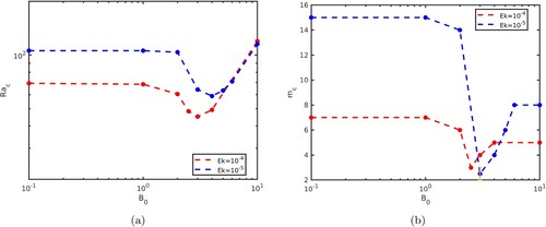
Table 1. Critical Rayleigh number ${Ra}_c$ and azimuthal wavenumber $m_c$ obtained in our simulations for varying $B_0$ and $Ek$.

$B_0$	${Ra}_c$	$m_c$	${Ra}_a$	$m_a$
$Ek={10}^{-4}$
0	69.4	7	62.24	6.5
0.1	69.4	7
1	68.5	7
2	60.4	6
2.5	48.3	3
3	45.1	4
4	49.2	5
10	119.4	5
$Ek={10}^{-5}$
0	105.8	15	102.65	14.0
1	105.8	15
2	103.7	14
3	64.0	2, 3${}^{\ast }$
4	58.9	4
5	63.2	6
6	71.0	8
10	115.4	8

Note: The last two columns for $B_0=0$ indicate the theoretical values ${Ra}_a$ and $m_a$ obtained in the asymptotic study of non-magnetic rotating spherical convection of Dormy et al. (2004). ${}^{\ast }$The onset of the modes m = 2 and 3 is very close for $B_0=3$ and $Ek={10}^{-5}$, both having a critical Rayleigh number of 64.0.

Table 2. Frequency ω of the dominant mode $m_n$ for simulations at $Ra$ just above ${Ra}_c$ compared with the theoretical value of the non-magnetic thermal Rossby waves, ${\omega }_a$, calculated for the mode $m_n$ in the asymptotic study of Dormy et al. (2004) (see appendix B).

Case	$m_n$	ω	${\omega }_a$
$Ek={10}^{-4}$
$B_0=0$, $Ra=70$	7	131.8	131.0
$B_0=3$, $Ra=46$	4	40.1	234.8
$B_0=10$, $Ra=120$	5	46.5	200.2
$Ek={10}^{-5}$
$B_0=0$, $Ra=106$	15	669.7	659.4
$B_0=4$, $Ra=60$	4	66.4	1479.3
$B_0=10$, $Ra=116$	9	−180.8	1106.6

Note: A positive frequency means that the wave propagates in the prograde direction.

The evolution of ${Ra}_c$ and $m_c$ with $B_0$ is similar to that observed in the linear magnetoconvection study of Sakuraba (2002), which mainly focussed on the case of internal heating with no inner core and zero flux boundary condition at $r=r_o$. The main difference between their results and ours is that Sakuraba observed that the preferred mode at the onset is an axisymmetric mode for $B_0\in [1,2]$. This axisymmetric “polar” mode consists of a large-scale meridional circulation that crosses the equatorial plane and transports heat between the two hemispheres. The absence of this polar mode at the onset in our simulations is presumably due to our choice of inner core size and fixed temperature boundary conditions, as Sakuraba shows that the stability curve of the polar mode increases towards larger $Ra$ in these conditions.

The qualitative behaviour of ${Ra}_c$ is also similar to that expected from linear magnetoconvection in rotating planar geometry (Chandrasekhar 1961). In the case where rotation vector and imposed magnetic field are vertical, ${Ra}_c$ starts to decrease when $B_0=\mathrm{O}\left({Ek}^{1/6}\right)$, while the lengthscale of the convection switches to a system-size scale (Roberts and King 2013). This change corresponds to a change in the primary force balance from a viscously-dominated regime for $B_0<\mathrm{O}\left({Ek}^{1/6}\right)$, where the viscous force is needed to break the Proudman-Taylor constraint, to a magnetically-dominated regime, where the Lorentz force becomes sufficiently large to assume this role. For the modest values of $Ek$ considered here, the regime change is expected to occur around $B_0\approx {Ek}^{1/6}\approx 0.1$. In our configuration, we find that the regime change occurs for larger $B_0$, $B_0=\mathrm{O}\left(1\right)$, with no apparent dependence on $Ek$. However, our simulations are relatively coarse-grained in $B_0$, while $Ek$ only varies by a decade. We would therefore not be able to pick up an ${Ek}^{1/6}$ trend. In planar magnetoconvection, the minimum of ${Ra}_c$ occurs for $B_0=\mathrm{O}\left(1\right)$ and, in the limit $B_0\to \mathrm{\infty }$, ${Ra}_c$ scales as $B_0^2$ and the critical horizontal wavenumber as $B_0$ (Roberts and King 2013). In our spherical system, we also find that ${Ra}_c$ becomes independent of $Ek$ at large $B_0$, although we have too few data points to check the scaling with $B_0$. However, the critical wavenumber retains an $Ek$-dependence with no clear dependence on $B_0$.

Table 2 gives the frequency ω of the waves at the dominant azimuthal wavenumber $m_n$ for simulations with $Ra$ just above ${Ra}_c$. By dominant wavenumber, we mean the wavenumber corresponding to the peak in the power spectrum of the kinetic energy. The frequencies were obtained by calculating the azimuthal drift of the dominant mode in Hovmöller maps (longitude-time maps at a fixed radius in the equatorial plane) of the radial velocity. Note that any azimuthal drift due to the zonal velocity was subtracted to extract the frequency of the waves. The frequency can be compared with the expected frequency of thermal Rossby waves of azimuthal wavenumber $m_n$ at the onset of non-magnetic convection, which we estimate by using the theoretical values provided by the asymptotic study of Dormy et al. (2004) for our configuration (see appendix B). Outside the tangent cylinder (where the height of the outer sphere decreases outwards), thermal Rossby waves always propagate in the prograde direction and their frequency decreases for increasing azimuthal wavenumber. For $B_0=0$, ω is close to the theoretical frequency of the thermal Rossby waves. For $B_0>0$, ω is much slower than the frequency of the thermal Rossby waves, indicating that the Lorentz force plays a significant role in the propagation mechanism. Near the minimum of ${Ra}_c$ ($B_0=3$ and 4 for $Ek={10}^{-4}$ and ${10}^{-5}$ respectively), the increase of the frequency of the dominant mode $m_n=4$ when $Ek$ decreases is relatively weak compared with the increase expected for the thermal Rossby wave (scaling as ${Ek}^{-2/3}$ in the leading order asymptotics, see appendix B). For $B_0=10$ at $Ek={10}^{-5}$, the wave propagates in the retrograde direction, revealing the dominance of the Lorentz force (Finlay 2008). The force balance in these waves will be analysed in section 3.3 below.

3.2. 3D structure of the flow

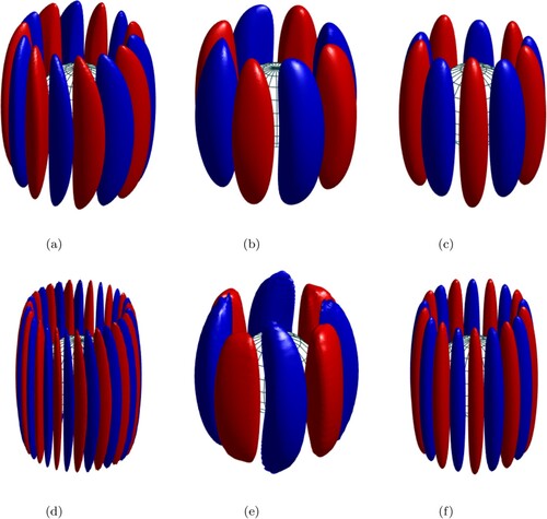
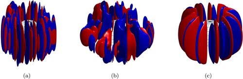
Figure 2 shows the 3D isosurfaces of the radial velocity $u_r$ for selected $B_0$ with $Ra$ just above the onset of convection for $Ek={10}^{-4}$ and ${10}^{-5}$. For each $Ek$, the three cases were chosen to represent the viscously-dominated regime ($B_0=0$) and the field-dominated regimes at the minimum of the ${Ra}_c$ stability curves ($B_0=3$ or 4) and at large $B_0$ ($B_0=10$). In all cases, the convective flow is mainly columnar. For $B_0=0$, we observe the well-known structure of thermal Rossby waves with a tilt of the column in the prograde direction (Zhang 1992). For $B_0\in [3,4]$, the flow adopts a banana shape with a visible z-dependence, especially for $Ek={10}^{-5}$. For $B_0=10$, the columns are straight with no tilt. The preservation of the columnar shape of the convection cells for $B_0>0$ can explain why the axial magnetic field starts to influence convection for $B_0=\mathrm{O}\left(1\right)$ in our simulations, while studies of spherical magnetoconvection with an imposed azimuthal field find that a smaller field amplitude ($B_0=\mathrm{O}\left({Ek}^{1/6}\right)$) is sufficient (Fearn 1979). In the axial field problem, the magnetic perturbations are created by the distortions of the imposed field due to the z-gradients of the velocity (via the $({\mathit{B}}_0\mathbf{\cdot }\mathbf{\nabla })\mathit{u}$ part of the induction term), as opposed to the azimuthal field problem, where they are mainly due to the ϕ-gradients. For columnar flows, the z-gradients of the velocity are much smaller than the ϕ-gradients, so the effect is only comparable for larger $B_0$.

Figure 2. Isosurfaces of $u_r$ for values of $Ra$ just above the onset of convection (as in table 2). The top row shows cases at $Ek={10}^{-4}$ and the bottom row at $Ek={10}^{-5}$. The red and blue surfaces correspond to isosurfaces at ±20$\mathrm{\%}$ of the maximum value of $u_r$ respectively. (a) $B_0=0$. (b) $B_0=3$. (c) $B_0=10$. (d) $B_0=0$. (e) $B_0=4$ and (f) $B_0=10$. (Colour online)

To study the axial structure of the flow, we consider the modified Proudman–Taylor constraint following Sakuraba (2002). Taking the curl of the Navier-Stokes equation (1(1) $\begin{array}{rl}\frac{\mathrm{\partial }\mathit{u}}{\mathrm{\partial }t}+\mathit{u}\mathbf{\cdot }\mathbf{\nabla }\mathit{u}+\frac{2}{Ek}{\mathit{e}}_z\times \mathit{u}& =-\frac{1}{Ek}\mathbf{\nabla }P+\frac{Ra}{Ek}\frac{r}{r_0}T{\mathit{e}}_r+\frac{1}{PmEk}\mathit{j}\times \mathit{B}+{\mathrm{\nabla }}^2\mathit{u},\end{array}$(1) ) and assuming that inertia, buoyancy and viscous forces are negligible gives (15) $\frac{\mathrm{\partial }}{\mathrm{\partial }z}(\mathit{u}+\frac{B_0}{2Pm}\mathit{j})\approx \mathbf{0},$(15) where the nonlinear contributions to the Lorentz force have also been neglected. Since the imposed field is uniform, $\mathit{j}$ is only produced by the induced magnetic field. We define the modified velocity as (16) $\hat{\mathit{u}}\equiv \mathit{u}+\frac{B_0}{2Pm}\mathit{j},$(16) so that the modified Proudman–Taylor constraint is $\mathrm{\partial }\hat{\mathit{u}}/\mathrm{\partial }z\approx \mathbf{0}$.

Figure 3 shows the s-components of $\mathit{u}$, $B_0/\left(2Pm\right)\mathit{j}$ and $\hat{\mathit{u}}$ on the axial cylindrical surface of radius s = 0.7 for the three cases of figure 2 at $Ek={10}^{-5}$. The onset of the dynamo for $B_0=0$ occurs at larger $Ra$ ($Ra\approx 500$) so this case does not have a magnetic field. For $B_0=4$, the contours of $u_s$ are bent along the z-axis, which gives the banana shape observed in 3D in figure 2. In this case, $B_0/\left(2Pm\right)j_s$ opposes $u_s$ near the equatorial region, which produces a modified velocity that is fairly z-invariant. The system therefore closely follows the modified Proudman–Taylor constraint (15(15) $\frac{\mathrm{\partial }}{\mathrm{\partial }z}(\mathit{u}+\frac{B_0}{2Pm}\mathit{j})\approx \mathbf{0},$(15) ). For $B_0=10$, both $u_s$ and ${\hat{u}}_s$ are largely z-invariant, although the deviation from z-invariance is greater near the outer boundary for the velocity. In this case, $B_0/\left(2Pm\right)j_s$ is greater near the outer boundary, where it is correlated with $u_s$. Interestingly, the axial structure of ${\hat{u}}_s$ for $B_0=4$ and 10 is similar to that of $u_s$ for $B_0=0$, with the maxima of the absolute value located near the outer boundary. This is perhaps logical, given that the increased significance of viscosity in the boundary layers acts to reduce the applicability of the (modified) Proudman–Taylor constraint there, allowing for local variations. Moreover $j_s$ has a contribution from $\mathrm{\partial }{B}_{\varphi }/\mathrm{\partial }z$, and since the magnetic boundary condition requires the toroidal scalar to go to zero at the outer radius, the maxima of $j_s$ at the boundary is also unsurprising. The fact that the maxima of $|u_s|$ are encountered around the equatorial region rather than near the outer boundaries (for $B_0>0$) has an effect on the convective heat transport, as shown in section 4.2.

Figure 3. Contour plots of $u_s$ (left), $B_0/\left(2Pm\right)j_s$ (middle) and ${\hat{u}}_s$ (right) on the axial cylindrical surface ($\varphi z$ plane) of cylindrical radius s = 0.7 for the three cases shown in figure 2 for $Ek={10}^{-5}$. For clarity, a restricted azimuthal range is shown; for (a), the azimuthal range is $\varphi \in [0,\pi /4]$, for (b) $\varphi \in [0,\pi ]$, and for (c) $\varphi \in [0,\pi /2]$. All panels on the same row have the same colorbar. (a) $B_0=0$, $Ra=106$. (b) $B_0=4$, $Ra=60$ and (c) $B_0=10$, $Ra=116$. (Colour online)

3.3. Force balance

To conclude this section, we investigate the dynamical force balance near the onset of convection. To do so, we look at the vorticity equation to eliminate the pressure term. Since the flow is mainly columnar, we consider the equation of the z-component of the vorticity ${\omega }_z$, (17) $\frac{\mathrm{\partial }{\omega }_z}{\mathrm{\partial }t}=I_C+I_L+I_B+I_V+I_R,$(17) where (18) $\begin{array}{rl}{I}_C& =\frac{2}{Ek}\frac{\mathrm{\partial }{u}_z}{\mathrm{\partial }z},\end{array}$(18) (19) $\begin{array}{rl}{I}_L& =\frac{1}{EkPm}[\mathbf{\nabla }\times (\mathit{j}\times \mathit{B}){]}_z,\end{array}$(19) (20) $\begin{array}{rl}{I}_B& =-\frac{Ra}{Ek{r}_o}\frac{\mathrm{\partial }T}{\mathrm{\partial }\varphi },\end{array}$(20) (21) $\begin{array}{rl}{I}_V& ={\mathrm{\nabla }}^2{\omega }_z,\end{array}$(21) (22) $\begin{array}{rl}{I}_R& =-[\mathbf{\nabla }\times (\mathit{u}\mathbf{\cdot }\mathbf{\nabla })\mathit{u}{]}_z.\end{array}$(22) Figure 4 shows ${\omega }_z$ and the terms in equations (18(18) $\begin{array}{rl}{I}_C& =\frac{2}{Ek}\frac{\mathrm{\partial }{u}_z}{\mathrm{\partial }z},\end{array}$(18) )–(22(22) $\begin{array}{rl}{I}_R& =-[\mathbf{\nabla }\times (\mathit{u}\mathbf{\cdot }\mathbf{\nabla })\mathit{u}{]}_z.\end{array}$(22) ) on the axial cylindrical surface of radius s = 0.7 for the three cases of figure 2 at $Ek={10}^{-5}$. The terms are plotted using individual snapshots that are representative of the flow over time. For $B_0=0$, the Coriolis and buoyancy terms are the most significant in the force balance; the viscous term is non-negligible, but is subdominant. Positive buoyancy terms are largely balanced by negative Coriolis terms, both being largest between anticyclones and cyclones (in the prograde direction); with opposite signs, there is a similar balance between cyclones and anticyclones. For $B_0=4$, the Lorentz term is one of the dominant forces, alongside the Coriolis and buoyancy terms (a MAC balance). The Coriolis and Lorentz terms balance each other at higher latitudes, whereas the contribution of the buoyancy term is more relevant near the equatorial region. Here, “sinks” in the buoyancy term are opposed by the Lorentz force, whilst buoyancy “sources” are balanced by the Coriolis force. For $B_0=10$, the force balance is primarily between the buoyancy term and the Lorentz term in the equatorial region (a MA balance), but towards the outer surface the balance is again between Coriolis and Lorentz contributions. The sum of the r.h.s. terms is relatively large for $B_0=0$, consistent with the greater frequency of propagation seen for that case in table 2. In other words, one effect of the Lorentz force for $B_0>0$ is to reduce this prograde propagation, as noted earlier for the frequencies at onset.

Figure 4. Contour plots, from left to right, of: ${\omega }_z$, $I_C$, $I_L$, $I_B$, $I_V$, $I_R$, and $I_T$=$I_C+I_L+I_B+I_V+I_R$ on the axial cylindrical surface ($\varphi z$ plane) of cylindrical radius s = 0.7 for the three cases shown in figure 2 for $Ek={10}^{-5}$. The second to sixth panels on each row have the same colorbar. For clarity, a restricted azimuthal range is shown; for (a), the azimuthal range is $\varphi \in [0,\pi /4]$, for (b) $\varphi \in [0,\pi ]$, and for (c) $\varphi \in [0,\pi /2]$. 10 radial grid points have been excluded at the outer boundary to highlight the dynamics in the bulk. (a) $B_0=0$, $Ra=106$. (b) $B_0=4$, $Ra=60$ and (c) $B_0=10$, $Ra=116$. (Colour online)

4. Evolution of the flow with increasing Rayleigh number

In the rest of paper, we will present results obtained at $Ek={10}^{-5}$ for varying $Ra$. Similar observations can be drawn from the simulations at $Ek={10}^{-4}$; exceptions are discussed in the text. In this section, we study how the presence of the ambient magnetic field affects the different components of the flow.

4.1. Convective flow

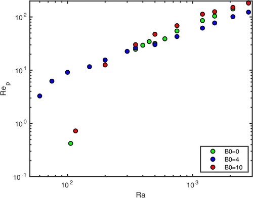
Figure 5 shows the evolution of the Reynolds number based on the poloidal velocity ${Re}_p$ (defined in equation (13(13) ${Re}_p={〈\sqrt{2E_k^p}〉}_t,$(13) )) as a function of $Ra$ for $B_0=0,4$ and 10. Cases with $B_0=4$ produce stronger ${Re}_p$ close to onset than cases with $B_0=0$ and 10. However, for $Ra$ away for the onset, there are no particularly notable differences in ${Re}_p$ for different $B_0$, although $B_0=4$ tends to produce slightly smaller ${Re}_p$. For the largest values of $Ra$, $B_0=0$ and $B_0=10$ produce ${Re}_p$ that become increasingly similar, to the point where the final values in the figure are overlapped. For $B_0=4$, a transition from a steady solution branch with dominant mode m = 4, to a branch with fluctuating solutions, is visible as a kink in the trend of ${Re}_p$ for $Ra>100$. (This transition is more prominent in some later plots of other diagnostics.)

Figure 5. Reynolds number of the poloidal flow as a function of the Rayleigh number for $Ek={10}^{-5}$. (Colour online)

The magnetic Prandtl number is set to 1 in all our simulations, so the magnetic Reynolds number $Rm$ is equal to the Reynolds number. In self-sustained spherical convective dynamos, the magnetic Reynolds numbers (based on the total velocity) needs to be greater than approximately 40 for dynamo action (Christensen and Aubert 2006). This is verified in our simulations with $B_0=0$, where the dynamo onsets at $Ra=500$ with a Reynolds number based on the total velocity of 73 and ${Re}_p=32$. Since the Reynolds number is essentially similar for all $B_0$ at a given $Ra$, we might consider that cases with $Ra>500$ for $B_0>0$ have magnetic Reynolds numbers that are large enough for dynamo action, so these solutions might behave essentially as dynamo solutions. This point will be explored in more detail in section 5.

To study the evolution of the columnar structure of the flow with $Ra$, we estimate the variations of the axial vorticity along z using the measure of the columnarity $C_{\omega z}$ proposed by Soderlund et al. (2012). $C_{\omega z}$ is based on the non-axisymmetric vorticity ${\mathit{\omega }}^{\prime }$ and defined as (23) $C_{\omega z}=\frac{\iint |〈{\omega }_z^{\prime }{〉}_z|s\mathrm{d}s\mathrm{d}\varphi }{\iint 〈|{\mathit{\omega }}^{\prime }|{〉}_{z}s\mathrm{d}s\mathrm{d}\varphi },$(23) where $〈\cdot {〉}_z$ denotes the average in the axial direction. The integral is evaluated as a sum on a discrete finite grid, where the summation is made over cylindrical radius s and ϕ outside the tangent cylinder. 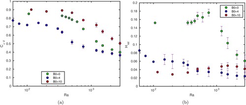This measure is calculated from taking the time average of $C_{\omega z}$ from various data snapshots. Figure 6(a) shows $C_{\omega z}$ as a function of $Ra$ for the same parameters as figure 5. The values of $C_{\omega z}$ near the onset of convection are consistent with our observations in section 3, i.e. the flow at $B_0=4$ ($B_0=10$) is less (more) z-invariant than for $B_0=0$. Soderlund et al. considered that the columnar structure breaks down when $C_{\omega z}<0.5$. By this definition, the columnar flows first breaks down for $B_0=4$ for $Ra\approx 350$. The degradation of the columnarity occurs later for $B_0=0$ and 10.

Figure 6. (a) Columnarity and (b) relative helicity as a function of $Ra$ for $Ek={10}^{-5}$. Both quantities have been time-averaged; the vertical bars shows the standard deviation. (Colour online)

Examples of the 3D structure of the flow are shown in figure 7 for $Ra=350$. As expected, the columnarity has visibly broken down for $B_0=4$, but the flow remains columnar to a good degree for $B_0=0$ and $B_0=10$. In this latter case, the flow displays quasi-2D sheet-like structures. Convection in this case is heterogeneous with quiescent regions located between the pair of intense radial jets. This sheet-like structure is still noticeable for higher values of $Ra$ but becomes less uniform between $Ra=500$ and $Ra=750$.

Figure 7. Isosurfaces of $u_r$ for (a) $B_0=0$, (b) $B_0=4$, and (c) $B_0=10$ at $Ra=350$ and $Ek={10}^{-5}$. The red and blue surfaces correspond to isosurfaces at ±20$\mathrm{\%}$ of the maximum value of $u_r$ respectively. (Colour online)

To further characterise the flow structure, we measure the kinetic helicity, which describes the spatial correlation between the components of the velocity and vorticity and is defined as (24) $H=\mathit{u}\mathbf{\cdot }\mathit{\omega }.$(24) The helicity is often thought to be essential to the generation of large-scale magnetic fields (Olson et al. 1999, Sreenivasan and Jones 2011, Moffatt and Dormy 2019) and is therefore an interesting measure to assess the dynamo capability of the flow. Since we study the evolution of the flow with varying $Ra$, we use the relative helicity defined as (Olson et al. 1999) (25) $H_{\mathrm{r}\mathrm{e}\mathrm{l}}=〈\mathit{u}\mathbf{\cdot }\mathit{\omega }{〉}_h/(〈\mathit{u}\mathbf{\cdot }\mathit{u}{〉}_h〈\mathit{\omega }\mathbf{\cdot }\mathit{\omega }{〉}_h{)}^{1/2},$(25) where $〈\cdot {〉}_h$ corresponds to the average in the northern or southern hemispheres. Similarly to $C_{\omega z}$, the measure is calculated from taking the time average from different data snapshots. $H_{\mathrm{r}\mathrm{e}\mathrm{l}}$ is negative (positive) in the northern (southern) hemispheres (Olson et al. 1999), so we average the absolute value of the two hemispheres. Figure 6(b) shows $H_{\mathrm{r}\mathrm{e}\mathrm{l}}$ as a function of $Ra$. For $B_0=0$, the relative helicity is approximately constant for non-magnetic solutions ($Ra<500$). There is a small increase in the helicity after the onset of dynamo action, while the saturated field remains weak (for $500\le Ra\le 750$, where $\Lambda <1$; see section 5); but for higher $Ra$ the helicity decreases significantly. After the columnarity breaks down, the time-averaged helicity in each of the two hemispheres remains approximately equal in absolute value. Around 50$\mathrm{\%}$ of the relative helicity is produced by the correlation of the z-components, $〈u_z{\omega }_z{〉}_h$. This percentage decreases slightly at the highest values of $Ra$, coinciding with the decrease in columnarity. Although the correlation of the z-components is always the largest contributor to the relative helicity, the dominance of the z-components is not as great as might naively be expected. In their asymptotic (small $Ek$) linear magnetoconvection analysis (with an imposed azimuthal field), Sreenivasan and Jones (2011) note that the contributions from $u_z{\omega }_z$ and $u_s{\omega }_s$ are equal. Nevertheless some authors (e.g. Soderlund et al. 2012) concentrate on the “axial helicity”, $u_z{\omega }_z$; and indeed, the variations in this quantity are informative. In the presence of an imposed axial field (for $B_0=4$ and 10), the correlation between $u_z$ and ${\omega }_z$ is poor, and the values of the relative helicity are always small. One possible consequence is that these flows would be inefficient for the generation of large-scale magnetic fields (in the absence of the imposed field). This is in contrast to the conclusions of Sreenivasan and Jones (2011), who found enhanced correlation of $u_z$ and ${\omega }_z$ (and thus enhanced helicity), from calculations with no imposed field, and also from linear magnetoconvection analysis with an imposed azimuthal field. (Most of their calculations used stress-free boundary conditions, where this effect is stronger; but the effect is also present with no-slip conditions, as in the calculations presented here.) They note the effect as stronger for solutions of dipolar symmetry (i.e. $B_r$ antisymmetric with respect to reflection in the equator), and argue that this effect may explain the dominance of this symmetry for planetary dynamos. Our imposed vertical field has this equatorial symmetry, but the Lorentz force produced by magnetoconvection in its presence clearly does not enhance the vertical flow within convective columns (and hence the helicity) in the same way. In the study of Sreenivasan and Jones, the Lorentz force was dominated by $B_{\varphi }$, which is zero near the equator so cannot balance the buoyancy force there. The Coriolis force must therefore balance the buoyancy force near the equator, meaning that the z derivative of $u_z$ cannot be zero there, giving rise to coherent axial flows along the columns. In our case the Lorentz force is dominated by $B_z$, so the buoyancy and Lorentz forces are able to balance near the equator.

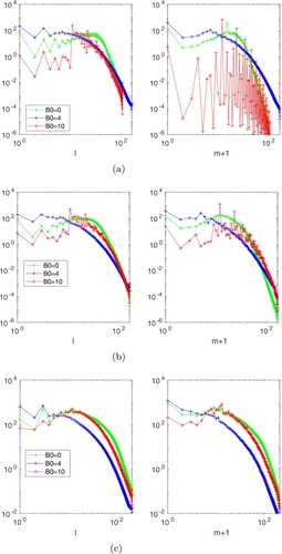
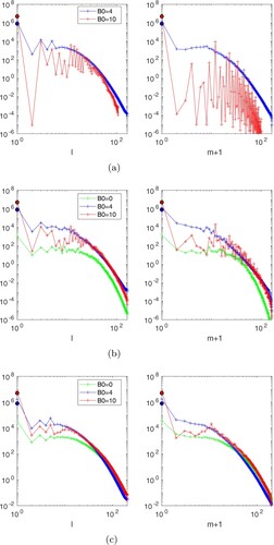
Figure 8 shows the spectra of the kinetic energy with respect to the spherical harmonic degree and order for selected Rayleigh numbers. For $B_0=0$ and 10, the peak of the spectra in m always remains close to their respective critical mode at the onset of convection. For $B_0=0$, there is no drastic change in the spectra for the non-magnetic ($Ra=350$) and dynamo ($Ra=750$) cases, except for a slight shift of the dominant m towards smaller values. For $B_0=4$, the peak is broader, even close to onset, and the energy is increasingly transferred to smaller azimuthal wavenumbers for increasing $Ra$.

Figure 8. Spectra of the kinetic energy with respect to the spherical harmonic degree l (left) and order m (right) for $Ek={10}^{-5}$. The spectra are time-averaged. (a) $Ra=350$. (b) $Ra=500$ and (c) $Ra=1200$. (Colour online)

Finally, we conclude this section by looking at the activity inside the tangent cylinder. Convection inside the tangent cylinder onsets when $750<Ra<1200$ for $B_0=0$. The convection begins at the edge of the tangent cylinder, encroaching from the convection flows in the rest of the shell, before spreading to all latitudes as $Ra$ increases. The delay of the convection onset inside the tangent cylinder is well-documented in studies of non-magnetic convection (Jones 2015) and is caused by the hindering effect of rotation on the linear onset, which is more pronounced towards the poles, where the direction of gravity and the rotation axis are aligned. For $B_0=4$, the convection onsets inside the tangent cylinder earlier than for $B_0=0$ (when $350<Ra<500$); in this case, the presence of both rotation and an imposed field with Elsasser number of order unity is favourable to convection, similarly to the situation outside the tangent cylinder. For $B_0=10$, convection has not occurred inside the tangent cylinder for the highest values of $Ra$ that we have considered ($Ra=2800$). This delay is also expected from results of linear magnetoconvection in plane layer geometry with no rotation or high Elsasser number (Chandrasekhar 1961): analogously to the rotating case, the hindering effect of the magnetic field on the convection onset is more pronounced towards the poles when the direction of the imposed field is aligned with the direction of gravity.

4.2. Efficiency of the heat transfer

We now study whether the changes to the 3D structure of the radial velocity for varying $B_0$ affect the efficiency of the heat transfer. We calculate the convective heat flux as (26) $\overline{F}=Pr\overline{u_{r}T},$(26) where the overbar denotes an azimuthal average. Contour plots of $\overline{F}$ are shown in figure 9 for $Ra$ near the onset of convection. Note that these cases are not exactly located at the same $Ra/{Ra}_c$, so we compare the shape of the contours rather than the amplitude of $\overline{F}$, and check that our observations remain valid for varying $Ra$ around these values. $\overline{F}$ occupies a wider region around the equatorial plane for $B_0=4$ than for both $B_0=0$ and 10. The Lorentz force partially offsets the Coriolis force in this region (figure 4), favouring more vigorous radial flow there.

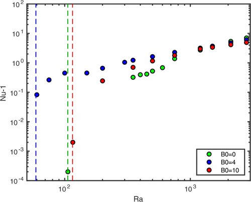
To measure the improved convective heat transfer in the presence of the imposed field, we look at the evolution of the Nusselt number (defined in equation (14(14) $Nu=-\frac{1}{\chi }{\frac{\mathrm{\partial }{〈T〉}_S}{\mathrm{\partial }r}|}_{r_o},$(14) )) with $Ra$ in figure 10. $Nu-1$ is approximately 2 orders of magnitude larger near the onset for $B_0=4$ than for $B_0=0$ and 10, so the efficiency of the convection is greatly improved near onset. As $Ra$ increases to values greater than 1000, the three cases tend to similar values of $Nu-1$. (Note that this is despite the slightly smaller ${Re}_p$ values noted for $B_0=4$ at high $Ra$; i.e. notwithstanding the relatively lower ${Re}_p$, the $B_0=4$ flow remains efficient at transferring heat.) This is somewhat surprising given the differences observed in the kinetic energy spectra at larger Rayleigh numbers, and in particular, that the flow is dominated by different lengthscales (this remains true at our largest Rayleigh number). This shows that global diagnostics such as ${Re}_p$ and $Nu$ do not fully capture the significant differences observed in the flow at large $Ra$. In all cases, the measure of columnarity indicates that the columnar structure has nearly broken down for these Rayleigh numbers for all three $B_0$, which could allow equally vigorous convection in all 3 cases. There has been considerable discussion of the variation of the heat flow in simulations (and experiments), and on its scaling with varying $Ra$, $Pr$ and $Ek$ (see Jones 2015, for a review and for references).

Figure 9. Meridional slices of the axisymmetric convective heat flux $\overline{F}$ for the three cases shown in figure 2 for $Ek={10}^{-5}$. (a) $B_0=0$. (b) $B_0=4$ and (c) $B_0=10$.

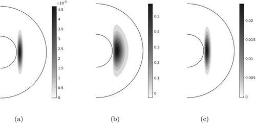
Figure 10. Nusselt number as a function of $Ra$ for $Ek={10}^{-5}$. The vertical dashed lines show the onset of convection for each case following the colour code of the legend. (Colour online)

4.3. Zonal flow

Dynamo simulations tend to have relatively weak zonal (i.e. axisymmetric azimuthal) flows compared with non-magnetic convection simulations (Aubert 2005), unless heterogeneous boundary conditions are used (Aubert et al. 2013). This is caused by the action of the Lorentz force to prevent the shearing of the poloidal field. We assess how the presence of an imposed axial magnetic field affects this behaviour. Figure 11 shows the ratio of the kinetic energy of the zonal flows to the total kinetic energy as a function of $Ra$. For $B_0=0$, the zonal flow amplitude is visibly reduced when the dynamo starts at $Ra=500$, as expected from previous dynamo studies. This ratio is much stronger for $B_0=4$ than for the other cases, reaching up to $30\mathrm{\%}$ for $Ra=200$. The strong axial field for $B_0=10$ largely suppresses zonal flows, whose energy remains around $1\mathrm{\%}$ only of the total kinetic energy.

Figure 11. Ratio of the kinetic energy of the zonal flows to the total kinetic energy as a function of $Ra$ for $Ek={10}^{-5}$. (Colour online)

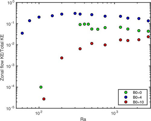
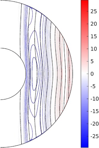
Figure 12 shows a meridional slice of the zonal flow for the case $B_0=4$ and $Ra=200$. The zonal flow is retrograde near the inner core and prograde near the outer boundary, which is a similar to the pattern observed in non-magnetic rotating spherical convection at moderate $Ra$ (Christensen 2002). The zonal flow has a strong degree of axial dependence in the region of the convective columns, with the largest amplitude near the equatorial region. Ferraro's law of isorotation (Ferraro 1937) states that, in the limit of high electrical conductivity (high $Rm$), the field lines of the time-averaged axisymmetric poloidal field lines and the isocontours of the time-averaged angular velocity, $\overline{u_{\varphi }}/s$, adjust to become aligned, thereby minimising the production of an azimuthal magnetic field via an omega effect (see e.g. Roberts 2015). To check the validity of Ferraro's law in our simulations, we superpose the axisymmetric poloidal magnetic field lines in figure 12. While the poloidal field remains largely directed along z, the z-dependence of the zonal flow means that the isocontours of the zonal flow cross the poloidal field lines around the mid-latitudes. This is at odds with Ferraro's law, but is not unexpected for a fluid of finite electrical conductivity.

Figure 12. Meridional slice of the zonal flow (colour) and field lines of the axisymmetric poloidal field (black lines) for $B_0=4$, $Ra=200$ and $Ek={10}^{-5}$. The zonal flow and the poloidal field have been time-averaged. (Colour online)

The presence of strong zonal flows for $B_0=4$ is surprising because the convective columns near the onset of convection do not have a tilt as for $B_0=0$. In the non-magnetic case, the column tilt produces the correlation between radial and azimuthal velocities, leading to significant Reynolds stresses that generate the zonal flows (Busse and Hood 1982). We therefore anticipate that the Reynolds stresses are not the primary source for the zonal flows for $B_0=4$. To determine the sources and sinks of the zonal kinetic energy for $B_0=4$, we examine the power budget for the zonal flow, following Aubert (2005). To do so, we multiply the azimuthal average of the ϕ-component of the Navier-Stokes equation (1(1) $\begin{array}{rl}\frac{\mathrm{\partial }\mathit{u}}{\mathrm{\partial }t}+\mathit{u}\mathbf{\cdot }\mathbf{\nabla }\mathit{u}+\frac{2}{Ek}{\mathit{e}}_z\times \mathit{u}& =-\frac{1}{Ek}\mathbf{\nabla }P+\frac{Ra}{Ek}\frac{r}{r_0}T{\mathit{e}}_r+\frac{1}{PmEk}\mathit{j}\times \mathit{B}+{\mathrm{\nabla }}^2\mathit{u},\end{array}$(1) ) by $\overline{u_{\varphi }}$ to obtain (27) $\frac{1}{2}\frac{\mathrm{\partial }{\overline{u_{\varphi }}}^2}{\mathrm{\partial }t}=P_R+P_C+P_L+P_V,$(27) where (28) $\begin{array}{rl}{P}_R& =-\overline{\left[\right(\mathit{u}\mathbf{\cdot }\mathbf{\nabla })\mathit{u}{]}_{\varphi }}\mathbf{\cdot }\overline{u_{\varphi }},\end{array}$(28) (29) $\begin{array}{rl}{P}_C& =-\frac{2}{Ek}\overline{u_s}\mathbf{\cdot }\overline{u_{\varphi }},\end{array}$(29) (30) $\begin{array}{rl}{P}_L& =\frac{1}{EkPm}\overline{[\mathit{j}\times \mathit{B}{]}_{\varphi }}\mathbf{\cdot }\overline{u_{\varphi }},\end{array}$(30) (31) $\begin{array}{rl}{P}_V& =\overline{[{\mathrm{\nabla }}^2\mathit{u}{]}_{\varphi }}\mathbf{\cdot }\overline{u_{\varphi }}.\end{array}$(31) Fi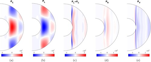gure 13 shows the time average of each of these terms in a meridional slice for the case $B_0=4$ and $Ra=200$. The power budget is dominated by the contributions from the Coriolis and Lorentz terms, which nearly balance each other, with the Lorentz term acting mainly as a sink near the equatorial region and a source towards mid-latitude. The contribution from the Reynolds stresses is small and acts as a sink around the tangent cylinder and a source at larger cylindrical radius, producing a mostly invariant pattern along z (and opposing the residual of $P_L+P_C$). The viscous term is a sink term in most of the domain, especially in the vicinity of the tangent cylinder and in the boundary layers (which have been excluded from figure 13 to highlight the dynamics in the bulk). Overall, the main sources of the zonal flow are the Coriolis and Lorentz forces, with contributions that are spatially-dependent. To complete the description of the source terms of the zonal flow, we analyse the terms in the thermal wind equation. The thermal wind equation is obtained by taking the azimuthal average of the ϕ-component of the curl of Navier-Stokes equation (1(1) $\begin{array}{rl}\frac{\mathrm{\partial }\mathit{u}}{\mathrm{\partial }t}+\mathit{u}\mathbf{\cdot }\mathbf{\nabla }\mathit{u}+\frac{2}{Ek}{\mathit{e}}_z\times \mathit{u}& =-\frac{1}{Ek}\mathbf{\nabla }P+\frac{Ra}{Ek}\frac{r}{r_0}T{\mathit{e}}_r+\frac{1}{PmEk}\mathit{j}\times \mathit{B}+{\mathrm{\nabla }}^2\mathit{u},\end{array}$(1) ) (e.g. Aubert 2005). 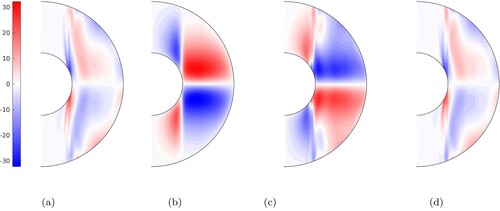Retaining only the Coriolis, buoyancy and Lorentz terms, we obtain (32) $\frac{\mathrm{\partial }\overline{u_{\varphi }}}{\mathrm{\partial }z}\approx \frac{Ra}{2r_o}\frac{\mathrm{\partial }\overline{T}}{\mathrm{\partial }\theta }-\frac{1}{2Pm}\overline{[\mathbf{\nabla }\times (\mathit{j}\times \mathit{B}){]}_{\varphi }}.$(32) Figure 14 shows the time average of each term in this equation for $B_0=4$ and $Ra=200$. The magnetic wind (driven by the Lorentz term) nearly balances the thermal wind (driven by the buoyancy term). The sum of the two terms is shown in plot (d) for comparison with the z-gradient of $\overline{u_{\varphi }}$ shown in plot (a). The two plots are nearly identical, which indicates that the viscous and nonlinear inertial terms only play a minor role in the balance. The thermal wind is stronger near the equatorial plane, while the magnetic wind is stronger close to the outer boundary. The magnetic wind is mainly due to the interaction of the magnetic perturbations with the imposed field and opposes the shearing of the poloidal magnetic field lines by the z-gradients of the zonal flow. The thermal wind is strong in this case because the convection is efficient at transporting heat as described in section 4.2, which creates strong latitudinal variations of the temperature. The enhanced zonal flows observed for $B_0=4$ (shown in figure 12) are therefore indirectly produced by the enhanced convective transport.

Figure 13. Time averages of the terms in the power budget of the zonal flow in a meridional slice for the same case as in figure 12. Ten radial points have been excluded at the inner and outer boundaries. (Colour online)

Sakuraba (2007) studied a case of magnetoconvection with imposed axial field for $Ek\approx {10}^{-5}$, $Ra\approx 500$ and $B_0\approx 1.4$ (where we have rescaled their parameters to match our definitions). They also observe the formation of thermal-wind driven zonal flows that are retrograde near the inner core. This is despite the different choice of thermal boundary conditions, with Sakuraba using mixed boundaries (fixed temperature at the inner core $r=r_i$ and zero flux at $r=r_o$). The shape of the isotherms are very sensitive to the choice of thermal boundary conditions, but the same choice of inner boundary condition seems to result in similar behaviour here, regardless of the differing outer condition.

Figure 14. Time averages of the terms in the thermal wind equation in a meridional slice for the same case as in figure 12. Plot (d) shows the sum of the buoyancy term and the Lorentz term. All the panels have the same colorbar. Ten radial points have been excluded at the inner and outer boundaries. (a) $\frac{\mathrm{\partial }\overline{u_{\varphi }}}{\mathrm{\partial }z}$. (b) $\frac{Ra}{2r_o}\frac{\mathrm{\partial }\overline{T}}{\mathrm{\partial }\theta }$. (c) $-\frac{1}{2Pm}(\overline{\mathbf{\nabla }\times (\mathit{j}\times \mathit{B})}{)}_{\varphi }$ and (d) Residual. (Colour online)

5. Generation of the magnetic field

5.1. Evolution of the magnetic energy with $Ra$

In this section, we study the characteristics of the magnetic field induced by the flow for varying $Ra$ and $B_0$. We first study the evolution of the strength of the magnetic field.

Figure 15(a) shows the Elsasser number $\Lambda$ (see definition in section 2.3) as a function of $Ra$. For $B_0=0$, the Elsasser number increases monotonically up to values greater than 1 for $Ra>1000$. For $Ek={10}^{-5}$, the magnetic field always remains dominated by the dipole in the range of Rayleigh numbers investigated here, which goes up to $Ra=2800$. Higher values of $Ra$ are required to enter the multipolar regime (Christensen and Aubert 2006). For $Ek={10}^{-4}$, the multipolar regime is entered at smaller values of $Ra$ ($Ra=2100$), at which point the Elsasser number decreases below unity. When $B_0>0$, $\Lambda$ drops towards ${\Lambda }_0$ ($=B_0^2$) near the onset of convection, so the solution branch is continuous at $Ra={Ra}_c$. For $B_0=4$, Λ reaches a local maximum for $Ra=100$, before increasing monotonically for $Ra>150$. This local maximum corresponds to the kink in the plot of ${Re}_p$ observed in section 4.1, and is the result of a change of branch between $Ra=100$ and 150. For $B_0=10$, Λ increases steadily after the onset of convection.

Figure 15. (a) Elsasser number $\Lambda$, (b) ratio $\Lambda /{\Lambda }_0$, and (c) squared Alfvén number $A^2$ (see definition (12(12) $A^2=\rho \mu U^2/B^2,$(12) )), as a function of $Ra$ for $Ek={10}^{-5}$. (Colour online)

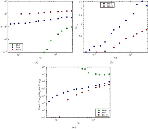
Figure 15(b) shows the ratio of $\Lambda /{\Lambda }_0$ as a function of $Ra$. The induced field exceeds the imposed field ($\Lambda /{\Lambda }_0>2$) for $B_0=4$ at $Ra>750$. For $B_0=10$, this situation has not yet occurred, although the amplitude of the induced field gets increasingly close to the imposed field: $\Lambda /{\Lambda }_0\approx 1.75$ for our largest Rayleigh number. For both $B_0=4$ and 10, there are no obvious changes in the evolution of $\Lambda$ around $Ra=500$, where the magnetic Reynolds number reaches the value of the dynamo threshold in the absence of imposed field.

Figure 15(c) shows the evolution of the squared Alfvén number, $A^2$, the ratio of the kinetic to magnetic energies as defined in section 2.3 (equation (12(12) $A^2=\rho \mu U^2/B^2,$(12) )). For reference, $A^2$ is thought to be of the order of ${10}^{-4}$ in the Earth's core (Aubert et al. 2017). For $B_0=0$, $A^2$ decreases with increasing $Ra$, but always remains fairly large, never falling below 0.1. For $B_0=4$ and 10, $A^2$ is much smaller, of the order of ${10}^{-5}$ and ${10}^{-7}$ close to the onset respectively. However, in both cases, $A^2$ increases with $Ra$ up to approximately ${10}^{-2}$ and $5\times {10}^{-3}$. The kinetic energy therefore increases more rapidly than the magnetic energy in the magnetoconvection case, contrary to the dynamo case.

Note that we did not observe notably large temporal fluctuations of the kinetic and magnetic energies in any of our simulations. For instance, at $Ra/{Ra}_c\approx 12$, the kinetic energy fluctuates by approximately $10\mathrm{\%}$ around the mean value, while the fluctuations of the magnetic energy tend to be smaller at larger $B_0$ (around $10\mathrm{\%}$ of the mean value for $B_0=0$ and $1\mathrm{\%}$ for $B_0=10$). 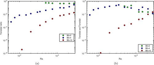Figure 16(a) shows the evolution of the toroidal ratio i.e. the ratio of the toroidal magnetic energy to the total magnetic energy. For $B_0=0$, the toroidal ratio is approximately 0.5 for all $Ra$. For $B_0>0$, the toroidal ratio is much smaller: simulations at $B_0=4$ slowly increases above 0.01 up to around 0.3, while for $B_0=10$, the toroidal ratio is less than ${10}^{-7}$ near the onset of convection and increases up to ${10}^{-2}$ for the largest $Ra$. The poloidal component therefore largely dominates the magnetic field in magnetoconvection with an imposed axial field, while the magnetic energy is equally distributed between poloidal and toroidal components in our dynamo simulations. This observation is consistent with the results of Sakuraba and Kono (2000).

Figure 16(b) shows the evolution of the ratio of the axisymmetric toroidal to the toroidal magnetic energies. For $B_0=0$, this ratio remains constant around 0.15 for the highest $Ra$. For $B_0=4$, approximately $50\mathrm{\%}$ of the toroidal magnetic energy is contained in the axisymmetric mode around $Ra=200$. This observation is consistent with the formation of strong zonal flows in this case, as the zonal flows distorts the poloidal magnetic field to produce the axisymmetric toroidal field via an omega effect. The zonal flows are relatively weaker at larger $Ra$, so the axisymmetric toroidal field weakens compared to the total toroidal field then. For $B_0=10$, the axisymmetric toroidal field is weak, especially at small $Ra$, which is consistent with the weak zonal flows observed in this case.

Figure 16. (a) Ratio of the toroidal magnetic energy to the total magnetic energy and (b) ratio of the axisymmetric toroidal to the toroidal magnetic energies as a function of $Ra$ for $Ek={10}^{-5}$. (Colour online)

To conclude this section, we study the partition of the poloidal magnetic energy between dipolar and multipolar components. Figure 17 shows the spectra of the time-averaged poloidal magnetic energy for fixed Rayleigh numbers. The dominant degree is l = 1 even for the highest values of $Ra$, indicating the dipolar nature of the field. As mentioned earlier, for $Ek={10}^{-4}$ at $B_0=0$, we found that the field becomes multipolar for $Ra=2100$, but no multipolar regime was found for $Ek={10}^{-5}$ for Rayleigh number up to $Ra=2800$. Christensen and Aubert (2006) found that convective dynamos produce multipolar fields when the local Rossby number (${Ro}_l=U/\left(\Omega L_u\right)$ with $L_u$ is a typical flow lengthscale) is greater than 0.1. In our simulations, ${Ro}_l\approx 0.03$ for $Ra=2800$ and $Ek={10}^{-5}$, so we expect that higher values of $Ra$ are required to enter the multipolar regime in this case, despite $C_{\omega z}$ being less than 0.5. The cases with $B_0>0$ show a gradual degradation of the relative dipole strength when $Ra$ increases, which is more pronounced for $B_0=4$. However, the field remains overwhelmingly dipolar even at large $Ra$ where the induced field is of the same order of magnitude as the imposed field. In these cases too, ${Ro}_l$ is still less than 0.1.

Figure 17. Spectra of the poloidal magnetic energy with respect to the spherical harmonic degree l (left) and order m (right) for $Ek={10}^{-5}$. The coloured circles on each vertical axis represent the poloidal energy of the imposed magnetic field itself. The spectra are time-averaged. (a) $Ra=350$. (b) $Ra=500$ and (c) $Ra=1200$. (Colour online)

5.2. Morphology of the magnetic field

We now analyse the morphology of the magnetic field, starting from the axisymmetric magnetic field. Figure 18 shows meridional slices of the axisymmetric azimuthal magnetic field and the poloidal magnetic field lines. In the magnetoconvective cases, the poloidal field lines remain largely z-invariant, indicating that the imposed field is relatively unperturbed by the induced poloidal field, with the most significant variations observed at larger $Ra$. For $B_0=4$ and $Ra=1200$, the induced field has a larger amplitude than the imposed field (see figure 15(b)) but, even then, the magnetic field largely retains the shape of the imposed magnetic field. For $B_0=4$, the azimuthal field consists of a single ring located outside the tangent cylinder and of opposite sign in each hemisphere. For $Ra=200$, the azimuthal field can be related to the zonal flow shown in figure 12 via an omega effect. Only weak azimuthal field is present inside the tangent cylinder, which is consistent with the absence of zonal flow there (and despite the presence of convection for $Ra\ge 500$). By contrast, for $B_0=0$, a strong azimuthal field is produced on the tangent cylinder and diffuses inwards (there is no convection inside the tangent cylinder for $Ra=500$ in this case). For $B_0=10$, the azimuthal field is very weak, even for higher values of $Ra$, and multiple patches are seen in both hemispheres.

Figure 18. Meridional slices of the axisymmetric azimuthal field (colour) and field lines of the axisymmetric poloidal field (black lines) for $Ek={10}^{-5}$. The magnetic field has been time-averaged in all cases. (a) $B_0=0$, $Ra=500$. (b) $B_0=4$, $Ra=200$. (c) $B_0=4$, $Ra=500$. (d) $B_0=4$, $Ra=1200$. (e) $B_0=10$, $Ra=200$. (f) $B_0=10$, $Ra=500$ and (g) $B_0=10$, $Ra=1200$.

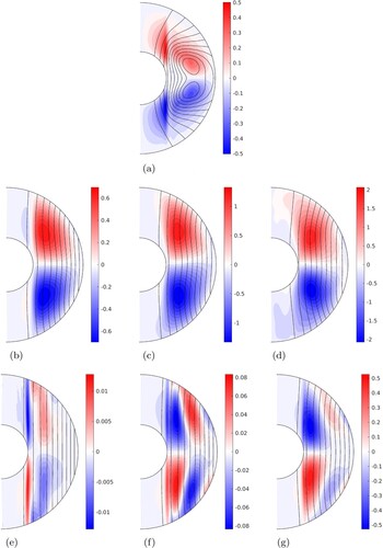
To determine whether the induced magnetic field reinforces or diminishes the imposed magnetic field, we plot in figure 19 the induced component of the axisymmetric axial magnetic field, $B_z-B_0$. Only the northern hemisphere is shown as $B_z$ is largely symmetric about the equator. For $B_0>0$, the axial magnetic field is strongest at higher latitudes, and of the sense to reinforce the imposed field. (The sense for $B_0=0$ is coincidental, as the opposite sense is an equally valid solution.) In the equatorial regions near the outer boundary (and in the exterior), the induced dipole field results in locally negative induced $B_z$ values; these are always weaker than the imposed field, however, so the total axisymmetric $B_z$ is always positive. For $B_0=4$, there is a significant octopole component of induced field close to onset, resulting in opposite polarity fields near the equator. At $Ra=500$, the induced field inside the tangent cylinder is a significant fraction of the imposed field. Overall, for both $B_0=4$ and 10, the induced axial dipole therefore reinforces the imposed field.

Figure 19. Meridional slices of the induced axisymmetric axial magnetic field, $B_z-B_0$, for $Ek={10}^{-5}$. The rows show cases at $B_0=0,4$ and 10 from top to bottom. The field has been time-averaged for $Ra=500$. (a) $Ra=500$. (b) $Ra=60$. (c) $Ra=500$. (d) $Ra=116$ and (e) $Ra=500$.

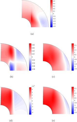
Figure 20 shows equatorial slices of the induced axial magnetic field (i.e. $B_z-B_0$) in the equatorial plane, superimposed on the axial vorticity. For $B_0=0$, we show the nearest case to the dynamo onset, $Ra=500\approx 4.7{Ra}_c^0$. In this case, the maximum of $B_z$ is located within the anticyclones, which is a familiar feature of convective dynamos (e.g. Jones 2011). In the magnetoconvective cases for Rayleigh numbers close to onset, the axial magnetic field is concentrated between cyclones and anticyclones, with regions of positive induced axial fields (which reinforce the imposed field) correlated with cold (inward) radial flow. At larger Rayleigh numbers ($Ra=350$) however, the axial magnetic field is concentrated in the anticyclones in the equatorial plane, similarly to the dynamo case. This observation is in agreement with the study of Sakuraba and Kono (2000) for ${\Lambda }_0>2$, which emphasises that the magnetic flux concentration inside anticyclones leads to an asymmetry between cyclones and anticyclones with enlarged anticyclones. They argue that the magnetic confinement is due to convergent flows towards the core of the anticyclones in the equatorial plane that compensate the Ekman pumping at the outer boundary.

Figure 20. Contours of the induced axial field $B_z-B_0$ (black lines) superimposed onto the axial vorticity (colour) in a quarter of the equatorial plane for cases at $Ek={10}^{-5}$. For the induced $B_z$, the solid and dashed lines denote positive and negative values respectively. The case for $B_0=0$ (a) is near the dynamo onset. Cases for $B_0>0$ are near the onset of convection (b)–(c) and for $Ra=350$ (d)–(e). Ten radial points have been excluded at the inner and outer boundaries to highlight the axial vorticity in the bulk of the fluid. (a) $B_0=0$, $Ra=500$. (b) $B_0=4$, $Ra=60$. (c) $B_0=10$, $Ra=116$. (d) $B_0=4$, $Ra=350$ and (e) $B_0=10$, $Ra=350$. (Colour online)

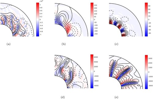
Figure 21. R.m.s. value of ${\overline{\mathcal{E}}}_{\varphi }^m$ as a function of m for the first 20 spherical harmonics orders. The red circle at m = 0 on each plot shows the value of ${\overline{\mathcal{E}}}_{\varphi }^0$ for the induced field only (i.e. $\mathit{B}-B_0{\mathit{e}}_z$). The values have been time-averaged for $Ra=500$. (a) $B_0=0$, $Ra=500$. (b) $B_0=4$, $Ra=60$. (c) $B_0=4$, $Ra=500$. (d) $B_0=10$, $Ra=116$ and (e) $B_0=10$, $Ra=500$. (Colour online)

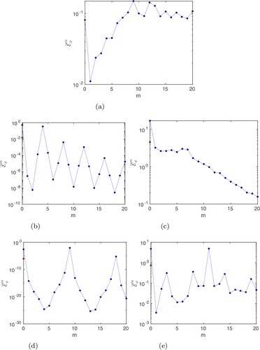
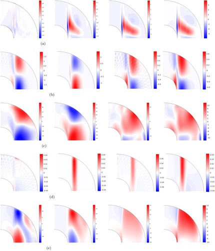
Figure 22. Meridional slices of ${\overline{\mathcal{E}}}_{\varphi }^m$ and $\overline{j_{\varphi }}$ for the same cases as in figure 21. The chosen values of m for ${\overline{\mathcal{E}}}_{\varphi }^m$ are noted in the subfigure caption. For the cases with $Ra=500$, the values have been time-averaged. (a) $B_0=0$, $Ra=500$; from left to right: ${\overline{\mathcal{E}}}_{\varphi }^0$, $\sum _{m=9}^{m=20}{\overline{\mathcal{E}}}_{\varphi }^m$, $\sum _{m=0}^{m=20}{\overline{\mathcal{E}}}_{\varphi }^m$, $\overline{j_{\varphi }}$. (b) $B_0=4$, $Ra=60$; from left to right: ${\overline{\mathcal{E}}}_{\varphi }^0$, ${\overline{\mathcal{E}}}_{\varphi }^4$, $\sum _{m=0}^{m=20}{\overline{\mathcal{E}}}_{\varphi }^m$, $\overline{j_{\varphi }}$. (c) $B_0=4$, $Ra=500$; from left to right: ${\overline{\mathcal{E}}}_{\varphi }^0$, $\sum _{m=1}^{m=8}{\overline{\mathcal{E}}}_{\varphi }^m$, $\sum _{m=0}^{m=20}{\overline{\mathcal{E}}}_{\varphi }^m$, $\overline{j_{\varphi }}$. (d) $B_0=10$, $Ra=116$; from left to right: ${\overline{\mathcal{E}}}_{\varphi }^0$, ${\overline{\mathcal{E}}}_{\varphi }^9$, $\sum _{m=0}^{m=20}{\overline{\mathcal{E}}}_{\varphi }^m$, $\overline{j_{\varphi }}$ and (e) $B_0=10$, $Ra=500$; from left to right: ${\overline{\mathcal{E}}}_{\varphi }^0$, ${\overline{\mathcal{E}}}_{\varphi }^{11}$, $\sum _{m=0}^{m=20}{\overline{\mathcal{E}}}_{\varphi }^m$, $\overline{j_{\varphi }}$. (Colour online)

5.3. Generation of the axisymmetric poloidal field

In order to determine which lengthscales play a major role in the generation of the axisymmetric poloidal magnetic field, we study the contributions to the electromotive force (e.m.f. ). The equation for the poloidal magnetic component $B_p$ is obtained by taking the dot product of the magnetic induction equation with the vector $\mathit{r}$, (33) $\frac{\mathrm{\partial }}{\mathrm{\partial }t}{L}_2{B}_p=\mathit{r}\mathbf{\cdot }\mathbf{\nabla }\times E+\frac{1}{Pm}{\mathrm{\nabla }}^2{L}_2{B}_p,$(33) where we have used that $r{B}_r=L_2{B}_p$ and the $L_2$ operator isolates the angular part of the Laplacian, (34) $L_2(\cdot )=-\frac{1}{\sin \theta }\frac{\mathrm{\partial }}{\mathrm{\partial }\theta }(\sin \theta \frac{\mathrm{\partial }(\cdot )}{\mathrm{\partial }\theta })-\frac{1}{{\sin }^2\theta }\frac{{\mathrm{\partial }}^2(\cdot )}{\mathrm{\partial }{\varphi }^2}.$(34) Applied to a spherical harmonic $Y_l^m$, it gives $L_2{Y}_l^m=l(l+1)Y_l^m$. The e.m.f. is $E=\mathit{u}\times \mathit{B}$. From equation (33(33) $\frac{\mathrm{\partial }}{\mathrm{\partial }t}{L}_2{B}_p=\mathit{r}\mathbf{\cdot }\mathbf{\nabla }\times E+\frac{1}{Pm}{\mathrm{\nabla }}^2{L}_2{B}_p,$(33) ), the axisymmetric poloidal component $\overline{B_p}$ is driven by the ϕ-component of the axisymmetric e.m.f., $\overline{{\mathcal{E}}_{\varphi }}$. (Specifically, the relevant source term is $(1/\sin \theta )\mathrm{\partial }(\sin \theta \overline{{\mathcal{E}}_{\varphi }})/\mathrm{\partial }\theta$.) We decompose $\overline{{\mathcal{E}}_{\varphi }}$ into contributions from individual azimuthal spherical harmonics order m, (35) ${\overline{\mathcal{E}}}_{\varphi }^m=\overline{u_r^m{B}_{\theta }^m}-\overline{B_r^m{u}_{\theta }^m},$(35) where the superscript indicates a component of the velocity or magnetic field corresponding to a given m.

Figure 21 shows the r.m.s. value of ${\overline{\mathcal{E}}}_{\varphi }^m$ as a function of m for $m\in [0,20]$ for $Ra$ close to onset and at $Ra=500$. Figure 22 shows the corresponding meridional slices of ${\overline{\mathcal{E}}}_{\varphi }^m$ for the dominant value(s) of m and also the sum $\sum _{m=0}^{m=20}{\overline{\mathcal{E}}}_{\varphi }^m$. $\overline{{\mathcal{E}}_{\varphi }}$ is mainly symmetric about the equator in all cases, so we only show the northern hemisphere. For comparison, we also plot the azimuthal component of the axisymmetric electric current (which is related to the mean e.m.f. via Ohm's law) (36) $\overline{j_{\varphi }}=\frac{1}{r}\frac{\mathrm{\partial }r\overline{B_{\theta }}}{\mathrm{\partial }r}-\frac{1}{r}\frac{\mathrm{\partial }\overline{B_r}}{\mathrm{\partial }\theta }.$(36) For $B_0=0$, the largest contribution to the mean e.m.f. is produced by the modes $m\ge 8$, all contributing at a similar level until m = 20. The large-scale modes $1\le m\le 7$ have relatively weak kinetic energy (see the kinetic energy spectrum in figure 8(b)), so it is perhaps unsurprising that their contribution to the mean e.m.f. is small. The sum of the mean e.m.f. produced by the modes $0\le m\le 20$ is very similar to $\overline{j_{\varphi }}$, so the small scales corresponding to m>20 only play a minor role in the generation of the axisymmetric poloidal field. In fact, this is true for all the cases shown in figure 22.

For $B_0=4$, the main contribution comes from m = 0 and m = 4 at onset, with m = 4 generating a mean e.m.f. that opposes that of m = 0 (which is largely due to the interaction of the axisymmetric meridional circulation with the imposed field), but cannot entirely match it. The net mean e.m.f. is thus similar to that of m = 0 with a reduced amplitude. It produces a ring of negative $\overline{j_{\varphi }}$ in the equatorial region, topped by a ring of positive $\overline{j_{\varphi }}$ at higher latitudes. Positive (negative) induced $B_z$ is produced inside (outside) the ring of positive $\overline{j_{\varphi }}$ and vice-versa (see figure 19). For $Ra=500$, modes up to m = 8 contribute significantly to ${\overline{\mathcal{E}}}_{\varphi }$. Here again the non-axisymmetric modes generate a mean e.m.f. in opposition to that of m = 0. The net e.m.f. now produces mainly a ring of positive $\overline{j_{\varphi }}$ whose maximum is located at mid-latitudes near the outer boundary. As a result, the induced $B_z$ is positive in most of the domain and only negative near the outer boundary at low latitudes. For $Ra$ away from the onset, the large-scale non-axisymmetric modes that dominate the kinetic energy spectrum (figure 8(b)) therefore largely contribute to the generation of an induced field that reinforces the imposed field.

At $B_0=10$ near onset, the dominant contribution comes from m = 9 (which dominates the kinetic energy spectrum). The resulting $\overline{j_{\varphi }}$ is positive and contained in a narrow band outside the tangent cylinder, which corresponds to the location of the columnar flow (see figures 2 and 20). Accordingly, the induced $B_z$ is mainly positive inside the tangent cylinder and negative outside. At higher $Ra$, the dominant non-axisymmetric mode is now m = 11 (also the dominant non-axisymmetric mode of the kinetic energy spectrum), with m = 0 contributing at a similar level. These two modes produce e.m.f. that are in opposition in most of the domain. As the flow structure extends further in cylindrical radius when $Ra$ increases (see figure 20), the resulting positive $\overline{j_{\varphi }}$ now fills most of the domain outside the tangent cylinder, producing a positive induced $B_z$ throughout most of the domain. Interestingly, the net mean e.m.f. is fairly similar for $B_0=4$ and $B_0=10$ at $Ra=500$ (hence similar induced $B_z$ in figure 19), although the contributions from individual modes are very different. This highlights a notable difference in field generation mechanisms between $B_0=4$ and $B_0=10$, although the net outcome in both cases is the production of an axisymmetric poloidal field reinforcing the imposed field in the interior.

6. Discussion

We have studied the effects of an imposed axial magnetic field ${\mathit{B}}_0=B_0{\mathit{e}}_z$ on rotating spherical convection at onset and for supercritical values of the Rayleigh number. Our parameter survey included both $Ek={10}^{-4}$ and $Ek={10}^{-5}$, for a range of values of $Ra/{Ra}_c$ varying from 1 to 50, with fixed $Pr=Pm=1$, and with fixed temperature, no-slip, and electrically insulating boundary conditions.

We found significant changes in the onset of convection when $B_0⪆\mathrm{O}\left(1\right)$ (where $B_0=1$ corresponds to an Elsasser number of unity), with a decrease in the critical Rayleigh number ${Ra}_c$ and azimuthal wavenumber $m_c$ that is more pronounced at small $Ek$. The critical Rayleigh number increases again for larger values of $B_0\sim \mathrm{O}\left(10\right)$, becoming independent of the choice of $Ek$. The structure of the flow at onset is mainly columnar, regardless of the choice of $B_0$. The primary force balance gradually changes as $B_0$ increases, and the Lorentz force becomes one of the dominant forces balancing the Coriolis and buoyancy forces. Interestingly, we find that the primary force balance varies locally: for $B_0=10$, the buoyancy and Lorentz forces balance in the equatorial region, but the balance is mainly between the Coriolis and Lorentz forces near the outer surface. The change in the force balance is evident in the wave propagation, which is prograde and matches the frequency of thermal Rossby waves for $B_0<\mathrm{O}\left(1\right)$, and subsequently slows down as $B_0$ increases, until reversing direction at $B_0=10$ for small $Ek$.

For higher values of $Ra$, the columnar flows break down, with the earliest collapse seen for $B_0=4$. In this case, more efficient transport of heat is seen in the equatorial region, as the Lorentz force offsets the Coriolis force here. The improved convective heat transfer leads to strong latitudinal variations of the temperature resulting in a strong thermal wind. This in turn has led to zonal flows in our magnetoconvective simulations, despite the equivalent dynamo simulations normally having weak zonal flows. These zonal flows can distort the poloidal component of the magnetic field, to produce a stronger axisymmetric toroidal field. For larger values of $B_0$, zonal flows are suppressed by the stronger axial field. Yadav et al. (2016b) found that the presence of dominant zonal flows (and hence large shear) in non-magnetic convection simulations reduces the efficiency of the convective heat transfer compared with dynamo cases, where the zonal flows are drastically reduced. This occurs when using stress-free boundary conditions, which favour the development of large zonal flows. Here, on the contrary, we have a strong thermal wind combined with efficient heat transfer. However the zonal flows are never dominant over the convective flows in our simulations because the zonal flow amplitude is limited by the use of no-slip boundaries. Additionally, Yadav et al. (2016b) found that no-slip dynamo simulations have significantly improved heat transfer compared with the non-magnetic cases when the Elsasser number of the self-sustained magnetic field is order unity, which is consistent with our results.

Near onset, the induced magnetic field generated by magnetoconvection is much smaller than the imposed field. The existence of subcritical behaviour, where a convective solution that is obtained by switching off the imposed field exists at the same parameters as the trivial conducting state, would require that the induced magnetic field is sufficiently strong to modify the flow effectively. Here we found that the field needs to be order unity to significantly influence the flow, so we expect that subcritical solutions would be difficult to maintain near onset. Indeed, we carried out multiple attempts to maintain convective dynamos below the onset of convection by gradually reducing the imposed field, but all were unsuccessful. However, for $B_0=4$, the induced field exceeds the imposed field for Rayleigh numbers approximately ten times critical. The induced field reinforces the imposed field in most of the domain, and the magnetic field largely retains the z-invariance of the imposed field, even at the largest Rayleigh numbers. The magnetically-modified flows are therefore able to generate a large-scale field with an intensity and morphology comparable to the imposed field. As a result, the intermittent behaviour observed in the planar dynamo simulations of Stellmach and Hansen (2004), Cooper et al. (2020) and suggested by the magnetoconvection results of Zhang and Gubbins (2000a, 2000b) might be avoided in this case. Additionally, hysteretic behaviour at high Rayleigh numbers might be possible: for Rayleigh numbers greater than the value required for the dynamo onset, a “strong” dynamo solution (obtained by switching off the imposed field) might exist at the same parameters as a “weak” dynamo solution (obtained by small initial perturbation). This was indeed observed by Sarson et al. (1997, 1999) and Sakuraba and Kono (2000) in this regime. We have also attempted to obtain hysteresis for $B_0=4$ and $Ra\ge 750$, but this has been unfruitful so far and will require further study.

The large-scale field generation is greatly affected by changes in the imposed field strength. In our dynamo simulations at $B_0=0$, the axisymmetric poloidal field is generated by the “small-scale” convective flows that are relatively unaffected by the Lorentz force (corresponding to azimuthal orders $m\in [8,20]$ for $Ek={10}^{-5}$, but we would expect these scales to become smaller for decreasing $Ek$ based on linear stability). A clear change occurs for $B_0=4$, where only the large-scale flows (with m<8) are significant in the production of the axisymmetric poloidal field. These scales carry most of the kinetic energy and are greatly affected by the Lorentz force. Notably, they lack attributes that are sometimes associated with the generation of axial dipoles (e.g. Olson et al. 1999, Sreenivasan and Jones 2011): their relative kinetic helicity and columnarity are significantly reduced compared with cases at $B_0=0$. Another change occurs at larger $B_0$ ($B_0=10$), where a single non-axisymmetric mode is largely responsible for the production of the axisymmetric poloidal field together with contributions from the axisymmetric mode (at least up to $Ra=500$, where this mode remains close to the value of the dominant wavenumber at onset). Our simulations are performed at moderate values of $Ek$, so the distinction between “small” and “large” scales is not strongly marked, but we would expect this distinction to become very pronounced in planetary core conditions at smaller $Ek$.

Magnetoconvection calculations help to elucidate the mechanisms for the production of magnetic fields in planets embedded in external fields of various strengths (e.g. the Jovian satellites and some exoplanets), as well as general aspects of field-generation in a strong-field regime. Our calculations complement the more prevalent studies of magnetoconvection with an imposed toroidal field. Some important differences are noted – including the imposed field strength required to markedly affect the flow (Fearn 1979) and the effect of the imposed axial field to reduce the relative kinetic helicity (e.g. see Sreenivasan and Jones 2011), with possibly significant implications for magnetic field generation – which warrant further work to elaborate to what extent the effects noted here rely on the imposed axial field geometry. A disadvantage of using a uniform magnetic field is that the whole domain is subject to the presence of the ambient field, whereas recent dynamo simulations show that the magnetic field is heterogeneous within the bulk of the domain (Schaeffer et al. 2017). The presence of magnetic-free regions have not been considered here, but could be the subject of future magnetoconvection studies. Other work could further investigate different boundary conditions or parameters, or imposing an axial field that is not uniform (Sreenivasan and Gopinath 2017).

Work is currently in progress to extend this study to variable $Pm$, for values both smaller and larger than the $Pm=1$ case considered here. The case $Pm<1$ is relevant to planetary interiors (where $Pm\ll 1$, based on molecular diffusivities); but as noted by Dormy (2016), the case $Pm>1$ may allow calculations at relatively high $Ek$ to attain a strong-field solution branch, more relevant to the expected magnetostrophic balance, than the weak-field and multipolar solutions found here for $Pm=1$ (when considering $B_0=0$). The combined effects of varying $Pm$ and $B_0$ are therefore of considerable interest for understanding planetary dynamos.

Acknowledgements

This research made use of the Rocket High Performance Computing service at Newcastle University and the DiRAC Data Intensive service at Leicester, operated by the University of Leicester IT Services, which forms part of the STFC DiRAC HPC Facility (www.dirac.ac.uk). DiRAC is part of the National e-Infrastructure. We thank the reviewers and editor whose comments helped clarify and improve the manuscript.

Disclosure statement

No potential conflict of interest was reported by the author(s).

Additional information

Funding

S.J.M. was supported by STFC studentship 2182079 under project ST/S505596/1. S.J.M. also gratefully acknowledges funding from the French government's Eiffel programme. C.G was supported by the UK Natural Environment Research Council under grant NE/M017893/1. The equipment was funded by BEIS capital funding via STFC capital grants ST/K000373/1 and ST/R002363/1 and STFC DiRAC Operations grant ST/R001014/1.

APPENDICES

Appendix A: Implementation of the externally imposed magnetic field

The magnetic field and electric current density, $\mathit{j}=\mathbf{\nabla }\times \mathit{B}$, are decomposed into poloidal and toroidal components (A.1) $\begin{array}{rl}\mathit{B}& =\mathbf{\nabla }\times \mathbf{\nabla }\times \left(B_p\mathit{r}\right)+\mathbf{\nabla }\times \left(B_t\mathit{r}\right),\end{array}$(A.1) (A.2) $\begin{array}{rl}\mathit{j}& =\mathbf{\nabla }\times \mathbf{\nabla }\times \left(j_p\mathit{r}\right)+\mathbf{\nabla }\times \left(j_t\mathit{r}\right).\end{array}$(A.2) The poloidal and toroidal scalars of $\mathit{B}$ and $\mathit{j}$ are related as (A.3) $j_p=B_t,j_t=-{\mathrm{\nabla }}^2{B}_p.$(A.3) In the vacuum outside the outer sphere, the electric current density is zero and so (A.4) $B_t=0,{\mathrm{\nabla }}^2{B}_p=0.$(A.4) The poloidal scalar is decomposed in spherical harmonics, (A.5) $B_p(r,\theta ,\varphi )=\sum _l\sum _m{g}_l^m\left(r\right)Y_l^m\mathrm{w}\mathrm{i}\mathrm{t}\mathrm{h}{Y}_l^m=C_l^m{\mathrm{P}}_l^m(\cos \theta ){\mathrm{e}}^{\mathrm{i}m\varphi }.$(A.5) Note that g here denotes the external solution, while we will denote the internal solution by p. ${\mathrm{\nabla }}^2{B}_p=0$ implies that (A.6) $r^2\frac{{\mathrm{d}}^2{g}_l^m}{\mathrm{d}{r}^2}+2r\frac{\mathrm{d}{g}_l^m}{\mathrm{d}r}-l(l+1)g_l^m=0,$(A.6) where we used $L_2{Y}_l^m=l(l+1)Y_l^m$, with $L_2$ the angular part of the Laplacian introduced in section 5.3. The solutions are of the form $g_l^m=C_{\alpha }{r}^{\alpha }$. Substituting in equation (A.6(A.6) $r^2\frac{{\mathrm{d}}^2{g}_l^m}{\mathrm{d}{r}^2}+2r\frac{\mathrm{d}{g}_l^m}{\mathrm{d}r}-l(l+1)g_l^m=0,$(A.6) ) gives $\alpha (\alpha +1)=l(l+1)$, which has for solutions $\alpha =l$ (corresponding to external sources) and $\alpha =-l-1$ (corresponding to internal sources).

We consider the case where an external source at $r>r_o$ produces a uniform axial field, (A.7) ${\mathit{B}}_0=B_0{\mathit{e}}_z=B_0\cos \theta {\mathit{e}}_r-B_0\sin \theta {\mathit{e}}_{\theta }.$(A.7) The imposed field only has a poloidal component. We denote by H and h the poloidal scalars of the imposed field in real and spectral spaces. The uniform axial field projects onto the spherical harmonics $(l,m)=(1,0)$ with the Legendre polynomial $P_1^0(\cos \theta )=\cos \theta$ and normalisation constant $C_1^0=\sqrt{3}$: (A.8) $H(r,\theta ,\varphi )=h_1^0\left(r\right)\sqrt{3}\cos \theta .$(A.8) By definition of the radial component of the field, $B_r=r^{-1}{L}_{2}H$, we get (A.9) $h_1^0\left(r\right)=\frac{B_0}{2\sqrt{3}}r.$(A.9) In the vacuum, the solution for the spherical harmonics $(l,m)=(1,0)$ is the contribution from the external and internal sources: (A.10) $g_1^0=\frac{B_0}{2\sqrt{3}}r+\frac{A}{r^2},$(A.10) where A is a constant. The poloidal scalar and its radial derivative are continuous at $r=r_o$, and so, the boundary condition for the internal solution at $r=r_o$ for $(l,m)=(1,0)$ is (A.11) $\begin{array}{rl}{p}_1^0\left(r_o\right)& =g_1^0\left(r_o\right),\end{array}$(A.11) (A.12) $\begin{array}{rl}{\frac{\mathrm{d}{p}_1^0}{\mathrm{d}r}|}_{r_o}& =\frac{B_0}{2\sqrt{3}}-\frac{2A}{r_o^3}=\frac{B_0}{2\sqrt{3}}-\frac{2}{r_o}\left(p_1^0\right(r_o)-\frac{B_0}{2\sqrt{3}}{r}_o)=-\frac{2}{r_o}{p}_1^0\left(r_o\right)+\frac{\sqrt{3}{B}_0}{2}.\end{array}$(A.12) There are no external sources for all the other spherical harmonics coefficients with $(l,m)\ne (1,0)$, so the external solution depending on $r^l$ must have $C_l=0$. For $(l,m)\ne (1,0)$, the boundary condition for the internal solution at $r=r_o$ is then simply (A.13) $\begin{array}{rl}{p}_l^m\left(r_o\right)& =g_l^m\left(r_o\right),\end{array}$(A.13) (A.14) $\begin{array}{rl}{\frac{\mathrm{d}{p}_l^m}{\mathrm{d}r}|}_{r_o}& ={\frac{\mathrm{d}{g}_l^m}{\mathrm{d}r}|}_{r_o}=-\frac{l+1}{r_o}{p}_l^m\left(r_o\right).\end{array}$(A.14) This latter boundary conditions is already implemented in PARODY, so the only required modification to the code is the implementation of the boundary condition (A.12(A.12) $\begin{array}{rl}{\frac{\mathrm{d}{p}_1^0}{\mathrm{d}r}|}_{r_o}& =\frac{B_0}{2\sqrt{3}}-\frac{2A}{r_o^3}=\frac{B_0}{2\sqrt{3}}-\frac{2}{r_o}\left(p_1^0\right(r_o)-\frac{B_0}{2\sqrt{3}}{r}_o)=-\frac{2}{r_o}{p}_1^0\left(r_o\right)+\frac{\sqrt{3}{B}_0}{2}.\end{array}$(A.12) ).

Appendix B: Theoretical frequency of the thermal Rossby waves

To compare the frequency of the waves near the onset of magnetoconvection in our simulations with the expected frequency of thermal Rossby waves at the same azimuthal wavenumber, we use the theoretical values for non-magnetic thermal Rossby waves provided by the asymptotic study of Dormy et al. (2004) in the case of differential heating with $\chi =0.35$ and no-slip boundaries. The theoretical values are given by (B.1) $\begin{array}{rl}{\omega }_a& =(1-\chi {)}^2[{\omega }^{gv}{\widehat{Ek}}^{-2/3}+{\widehat{Ek}}^{-1/3}{\left(\frac{\mathrm{\partial }\omega }{\mathrm{\partial }m}\right)}_c{m}_n],\end{array}$(B.1) (B.2) $\begin{array}{rl}{\omega }^{gv}& ={\omega }_c^{gv}+{\widehat{Ek}}^{2/9}{\omega }_1^{gv}+{\widehat{Ek}}^{1/6}{\tilde{\omega }}^{gv},\end{array}$(B.2) (B.3) $\begin{array}{rl}\widehat{Ek}& =Ek\frac{(1-\chi {)}^2}{2},\end{array}$(B.3) where we have introduced the relevant factors to match our choice of units and (B.4) ${\omega }_c^{gv}=0.743835,{\omega }_1^{gv}=0.56878,{\tilde{\omega }}^{gv}=-0.72723,{\left(\frac{\mathrm{\partial }\omega }{\mathrm{\partial }m}\right)}_c=-\mathrm{2.2637.}$(B.4) $m_n$ is the azimuthal wavenumber of the dominant mode in the numerical simulations.

Appendix C: List of simulations

Table C1. Summary of the input and output quantities for the simulations at $Ek={10}^{-5}$ and $Pr=Pm=1$.

$Ra$	$l_{max}$	$m_{max}$	$N_r$	$E_k$	$E_m$	$Nu$	$C_{\omega z}$	$H_{\mathrm{r}\mathrm{e}\mathrm{l}}$
$B_0=0$
106	84	64	120	0.34	0	1.000	0.852	0.152
350	108	108	160	1489.4	0	1.323	0.829	0.152
400	108	108	160	2191.9	0	1.395	0.816	0.153
450	164	164	160	3071.1	0	1.415	0.802	0.157
500	164	164	160	2691.8	0.048	1.524	0.7829	0.169
600	164	164	160	4116.0	0.079	1.685	0.7592	0.165
750	164	164	160	6733.6	0.41	2.385	0.6738	0.176
1200	204	204	200	13762	1.3	3.721	0.5277	0.132
1500	204	204	200	18620	2.2	4.675	0.4784	0.104
2100	204	204	200	31633	3.7	6.374	0.4302	0.075
2800	204	204	200	52062	4.9	8.010	0.4000	0.061
$B_0=4$
60	64	64	120	13.0	8.1	1.083	0.7744	0.086
75	64	64	120	49.5	8.4	1.263	0.7359	0.073
100	64	64	120	115.9	9.3	1.450	0.7204	0.059
150	108	108	120	241.2	9.3	1.452	0.7451	0.064
200	124	124	120	448.1	10.3	1.655	0.7188	0.060
300	164	164	120	963.3	12.7	2.045	0.6780	0.056
350	164	164	120	1263.4	13.9	2.229	0.6362	0.051
500	164	164	160	1629.7	15.0	2.627	0.5182	0.037
750	164	164	160	2942.0	17.6	3.272	0.4659	0.034
1200	204	204	200	6023.7	20.8	4.175	0.4217	0.033
1500	204	204	200	8625.0	26.0	4.699	0.4062	0.029
2100	204	204	200	14563	28.3	5.755	0.3848	0.025
2800	204	204	200	22261	25.4	7.048	0.3651	0.024
$B_0=10$
116	64	64	120	0.58	50.0	1.002	0.902	0.034
200	84	84	120	154.7	51.4	1.244	0.880	0.029
350	108	108	160	813.7	56.4	1.702	0.892	0.033
500	164	164	160	1940.6	62.7	2.160	0.865	0.041
750	204	204	200	4043.8	70.2	2.787	0.778	0.043
1200	204	204	200	10673	74.5	3.968	0.720	0.048
1500	204	204	200	14331	78.9	4.376	0.644	0.049
2100	204	204	200	22898	83.7	5.130	0.559	0.047
2800	204	204	200	34509	87.4	5.917	0.505	0.042

Note: $l_{max}$ and $m_{max}$ are the truncation degree and order of the spherical harmonics expansion and $N_r$ is the number of radial grid points. $E_k$ and $E_m$ are the volumetric kinetic and magnetic energies.

References

- Aubert, J., Steady zonal flows in spherical shell dynamos. J. Fluid Mech. 2005, 542, 53–67.
- Aubert, J., Aurnou, J. and Wicht, J., The magnetic structure of convection-driven numerical dynamos. Geophys. J. Int. 2008, 172, 945–956.
- Aubert, J., Finlay, C.C. and Fournier, A., Bottom-up control of geomagnetic secular variation by the Earth's inner core. Nature 2013, 502, 219–223.
- Aubert, J., Gastine, T. and Fournier, A., Spherical convective dynamos in the rapidly rotating asymptotic regime. J. Fluid Mech. 2017, 813, 558–593.
- Busse, F.H. and Hood, L.L., Differential rotation driven by convection in a rapidly rotating annulus. Geophys. Astrophys. Fluid Dyn. 1982, 21, 59–74.
- Cardin, P. and Olson, P., The influence of toroidal magnetic field on thermal convection in the core. Earth Planet. Sci. Lett. 1995, 132, 167–181.
- Chandrasekhar, S., Hydrodynamic and Hydromagnetic Stability, 1961 (Oxford: Oxford University Press).
- Cheng, J.S. and Aurnou, J.M., Tests of diffusion-free scaling behaviors in numerical dynamo datasets. Earth Planet. Sci. Lett. 2016, 436, 121–129.
- Christensen, U.R., Zonal flow driven by strongly supercritical convection in rotating spherical shells. J. Fluid Mech. 2002, 470, 115–133.
- Christensen, U.R. and Aubert, J., Scaling properties of convection driven dynamos in rotating spherical shells and application to planetary magnetic fields. Geophys. J. Int. 2006, 166, 97–114.
- Christensen, U.R. and Wicht, J., Numerical dynamo simulations. In Core Dynamics, 2nd ed., edited by P. Olson, Vol. 8 of Treatise on Geophysics, pp. 245–282, 2015 (Elsevier: Amsterdam).
- Christensen, U., Aubert, J., Cardin, P., Dormy, E., Gibbons, S., Glatzmaier, G., Grote, E., Honkura, Y., Jones, C., Kono, M., Matsushima, M., Sakuraba, A., Takahashi, F., Tilgner, A., Wicht, J. and Zhang, K., A numerical dynamo benchmark. Phys. Earth Planet. Inter. 2001, 128, 25–34.
- Cooper, R.G., Bushby, P.J. and Guervilly, C., Subcritical dynamos in rapidly rotating planar convection. Phys. Rev. Fluids 2020, 5, 113702.
- Dormy, E., Strong-field spherical dynamos. J. Fluid Mech. 2016, 789, 500–513.
- Dormy, E., Cardin, P. and Jault, D., MHD flow in a slightly differentially rotating spherical shell, with conducting inner core, in a dipolar magnetic field. Earth Planet. Sci. Lett. 1998, 160, 15–30.
- Dormy, E., Soward, A.M., Jones, C.A., Jault, D. and Cardin, P., The onset of thermal convection in rotating spherical shells. J. Fluid Mech. 2004, 501, 43–70.
- Fearn, D.R., Thermal and magnetic instabilities in a rapidly rotating fluid sphere. Geophys. Astrophys. Fluid Dyn. 1979, 14, 103–126.
- Fearn, D.R., Hydromagnetic waves in a differentially rotating annulus III. The effect of an axial field. Geophys. Astrophys. Fluid Dyn. 1985, 33, 185–197.
- Fearn, D.R. and Weiglhofer, W.S., Magnetic instabilities in rapidly rotating spherical geometries I. From cylinders to spheres. Geophys. Astrophys. Fluid Dyn. 1991a, 56, 185–197.
- Fearn, D.R. and Weiglhofer, W.S., Magnetic instabilities in rapidly rotating spherical geometries II. more realistic fields and resistive instabilities. Geophys. Astrophys. Fluid Dyn. 1991b, 60, 275–294.
- Fearn, D.R. and Weiglhofer, W.S., Magnetic instabilities in rapidly rotating spherical geometries. III. The effect of differential rotation. Geophys. Astrophys. Fluid Dyn. 1992a, 67, 163–184.
- Fearn, D.R. and Weiglhofer, W.S., Resistive instability and the magnetostrophic approximation. Geophys. Astrophys. Fluid Dyn. 1992b, 63, 111–138.
- Ferraro, V.C., The non-uniform rotation of the sun and its magnetic field. Mon. Not. R. Astron. Soc. 1937, 97, 458.
- Finlay, C.C., Waves in the presence of magnetic fields, rotation and convection. In Dynamos, edited by P. Cardin and L.F. Cugliandolo, Vol. 88 of Lecture Notes of the Les Houches Summer School, pp. 403–450, 2008 (Elsevier: Amsterdam).
- Gillet, N., Brito, D., Jault, D. and Nataf, H.C., Experimental and numerical studies of magnetoconvection in a rapidly rotating spherical shell. J. Fluid Mech. 2007, 580, 123–143.
- Gillet, N., Jault, D., Canet, E. and Fournier, A., Fast torsional waves and strong magnetic field within the Earth's core. Nature 2010, 465, 74–77.
- Gómez-Pérez, N. and Wicht, J., Behavior of planetary dynamos under the influence of external magnetic fields: Application to Mercury and Ganymede. Icarus 2010, 209, 53–62.
- Jones, C.A., Planetary magnetic fields and fluid dynamos. Annu. Rev. Fluid Mech. 2011, 43, 583–614.
- Jones, C.A., Thermal and compositional convection in the outer core. In Core Dynamics, 2nd ed., edited by P. Olson, Vol. 8 of Treatise on Geophysics, pp. 115–159, 2015 (Elsevier: Amsterdam).
- King, E.M. and Buffett, B.A., Flow speeds and length scales in geodynamo models: the role of viscosity. Earth Planet. Sci. Lett. 2013, 371, 156–162.
- Moffatt, K. and Dormy, E., Self-Exciting Fluid Dynamos, 2019 (Cambridge: Cambridge University Press).
- Olson, P. and Glatzmaier, G.A., Magnetoconvection in a rotating spherical shell: structure of flow in the outer core. Phys. Earth Planet. Inter. 1995, 92, 109–118.
- Olson, P.L., Christensen, U.R. and Glatzmaier, G.A., Numerical modelling of the geodynamo: mechanisms of field generation and equilibration.. J. Geophys. Res. 1999, 104, 10383–10404.
- Oruba, L. and Dormy, E., Predictive scaling laws for spherical rotating dynamos. Geophys. J. Int. 2014, 198, 828–847.
- Proctor, M.R.E., Convection and magnetoconvection in a rapidly rotating sphere. In Lectures on Solar and Planetary Dynamos, Publications of the Newton Institute, edited by M.R.E. Proctor and A.D. Gilbert, pp. 97–115, 1994 (Cambridge University Press: Cambridge).
- Roberts, P.H., Theory of the geodynamo. In Core Dynamics, 2nd ed., edited by P. Olson, Vol. 8 of Treatise on Geophysics, pp. 57–90, 2015 (Elsevier: Amsterdam).
- Roberts, P.H. and King, E.M., On the genesis of the Earth's magnetism. Rep. Progr. Phys. 2013, 76, 096801.
- Sakuraba, A., Linear magnetoconvection in rotating fluid spheres permeated by a uniform axial magnetic field. Geophys. Astrophys. Fluid Dyn. 2002, 96, 291–318.
- Sakuraba, A., A jet-like structure revealed by a numerical simulation of rotating spherical-shell magnetoconvection. J. Fluid Mech. 2007, 573, 89–104.
- Sakuraba, A. and Kono, M., Effect of a uniform magnetic field on nonlinear magnetoconvection in a rotating fluid spherical shell. Geophys. Astrophys. Fluid Dyn. 2000, 92, 255–287.
- Sarson, G.R., Jones, C.A., Zhang, K. and Schubert, G., Magnetoconvection dynamos and the magnetic fields of Io and Ganymede. Science 1997, 276, 1106–1108.
- Sarson, G.R., Jones, C.A. and Zhang, K., Dynamo action in a uniform ambient field. Phys. Earth Planet. Inter. 1999, 111, 47–68.
- Schaeffer, N., Efficient spherical harmonic transforms aimed at pseudospectral numerical simulations. Geochem. Geophys. Geosyst. 2013, 14, 751–758.
- Schaeffer, N., Jault, D., Nataf, H.C. and Fournier, A., Turbulent geodynamo simulations: a leap towards Earth's core. Geophys. J. Int. 2017, 211, 1–29.
- Soderlund, K.M., King, E.M. and Aurnou, J., The influence of magnetic fields in planetary dynamo models. Earth Planet. Sci. Lett. 2012, 333-334, 9–20.
- Sreenivasan, B. and Gopinath, V., Confinement of rotating convection by a laterally varying magnetic field. J. Fluid Mech. 2017, 822, 590–616.
- Sreenivasan, B. and Jones, C.A., Helicity generation and subcritical behaviour in rapidly rotating dynamos. J. Fluid Mech. 2011, 688, 5–30.
- Stellmach, S. and Hansen, U., Cartesian convection driven dynamos at low Ekman number. Phys. Rev. E 2004, 70, 056312.
- Teed, R.J., Jones, C.A. and Tobias, S.M., The transition to Earth-like torsional oscillations in magnetoconvection simulations. Earth Planet. Sci. Lett. 2015, 419, 22–31.
- Yadav, R., Gastine, T., Christensen, U., Wolk, S.J. and Poppenhaeger, K., Approaching a realistic force balance in geodynamo simulations. Proc. Natl. Acad. Sci. 2016a, 113, 12065–12070.
- Yadav, R.K., Gastine, T., Christensen, U.R., Duarte, L. and Reiners, A., Effect of shear and magnetic field on the heat-transfer efficiency of convection in rotating spherical shells. Geophys. J. Int. 2016b, 204, 1120–1133.
- Zhang, K., Spiralling columnar convection in rapidly rotating spherical fluid shells. J. Fluid Mech. 1992, 236, 535–556.
- Zhang, K., Spherical shell rotating convection in the presence of a toroidal magnetic field. Proc. R. Soc. Lond. A 1995, 448, 245–268.
- Zhang, K. and Fearn, D., How strong is the invisible component of the magnetic field in the Earth's core? Geophys. Res. Lett. 1993, 20, 2083–2086.
- Zhang, K. and Gubbins, D., Is the geodynamo process intrinsically unstable? Geophys. J. Int. 2000a, 140, F1–F4.
- Zhang, K. and Gubbins, D., Scale disparities and magnetohydrodynamics in the Earth's core. Phil. Trans. R. Soc. A 2000b, 358, 899–920.