Resonant growth of inertial oscillations from lee waves in the deep ocean

Abstract

The interactions between inertial oscillations (IO) and lee waves (LW) close to the bottom of the ocean and the role of IO in energy dissipation are addressed for a range of physical parameters typical of Southern Ocean conditions. Idealized numerical simulations in a vertical plane and resonant interaction theory are combined for this purpose. The lee waves are emitted by a uniform geostrophic flow over a sinusoidal topography for a constant buoyancy frequency at mid-latitude. We show that IO can grow by triadic resonant interactions with the LW. Two triads are dominant, which involve waves with frequency ${\omega }_{LW}$, f and ${\omega }_{LW}-f$, where ${\omega }_{LW}$ is the intrinsic frequency of the LW and f the Coriolis frequency (assumed positive). These triads differ by the sign and value of the IO vertical wavenumber. Results from the numerical simulations show that the triad associated with the upward phase propagation of the IO is selected, consistent with oceanic observations, that a good agreement is obtained with the IO growth rate predicted theoretically and that the IO develop in a bottom layer of height less than 1000 m. A quasi-steady flow regime is eventually reached, with the IO amplitude being of the same order as the geostrophic flow speed. During this regime, depending upon the flow parameters, the IO kinetic energy is equal to 30–70% of the LW energy flux during one inertial period. This large range of values is not reflected in the turbulent kinetic energy (TKE) dissipation rate, which is comprised between 10 and 30% of the LW energy flux, whatever the IO amplitude, even if vanishingly small. Therefore, for the set of parameters we consider, the TKE dissipation rate cannot be inferred from the IO amplitude. Yet, the nonlinear interactions between the lee waves and the IO are critical in setting the energy spectrum, and similarly for the internal tide and the IO at low latitudes according to the literature. This implies that IO should be taken into account in the parameterisation of mixing in the ocean.

Keywords:

• Deep ocean
• lee waves
• inertial oscillations
• resonant interactions
• dissipation

1. Introduction

Emission of internal gravity waves at a boundary by a steady mean flow, called lee waves (LW), has received considerable attention since the 1960s, pointing to the major impact of these waves on mean flows in the atmosphere. As reviewed by Bretherton (1969) already, the emission of LW results in a pressure (or drag) force on the topography in the direction of the mean flow. LW exert a force on the mean flow only when they break or dissipate. Indeed the waves transport momentum upwards up to the altitude where breaking occurs and the wave-induced momentum is deposited there, resulting in the deceleration of the mean flow (or its acceleration if the mean flow direction has changed at the breaking level). Momentum transfer to the mean flow also occurs at a critical level, where the wave frequency relative to that flow vanishes (Bretherton 1966).

In the ocean, by contrast, the interest in internal gravity waves lies primarily in their ability to mix the fluid via breaking. Mixing processes are indeed required to raise the deep cold water masses to the surface, as part of the meridional overturning circulation (Munk and Wunsch 1998), and the sources and locations of mixing are key questions in physical oceanography (Waterhouse et al. 2014). The mixing of the fluid and the wave-induced force on the fluid resulting from breaking are actually two facets of the same process: mixing results in the increase in the background potential energy of the flow while the wave-induced force is associated with a change in the distribution of the potential vorticity of the flow (e.g. McIntyre and Norton 1990). Concern about the latter force has recently been raised in the ocean and its role in the momentum balance of energetic regions questioned (Olbers and Eden 2017). There is also a growing interest in improving the representation of bottom drag (which includes the drag due to lee wave generation) in ocean circulation models considering the impact of this representation on large scale flow properties (Arbic et al. 2019).

Until the end of the 1990s, emission of LW was considered as unimportant in the ocean, the two main mechanical sources of internal gravity waves being the wind blowing at the sea surface and the tide flowing above seamounts and continental shelves (Munk and Wunsch 1998). However, field experiments have revealed the presence of strong mixing regions over rough topography at the bottom of the Southern Ocean, extending up to about one thousand metres above the bottom (Polzin and Firing 1997, Naveira Garabato et al. 2004). These observations and subsequent field campaigns in the Southern Ocean shaped a scenario of LW radiation by the Antarctic Circumpolar Current (ACC) and geostrophic eddies flowing over rough topography, resulting in momentum transport and breaking away from the topography. Subsequent estimates of the energy flux of LW in the ocean indicate that about 50% of that flux occurs in the Southern Ocean (Nikurashin and Ferrari 2011). Moreover, the power input from geostrophic motions into LW appears to be comparable (possibly only two times smaller) to that from the tide into the internal tide and from the wind to near-inertial oscillations (Waterhouse et al. 2014, Wright et al. 2014).

Near-inertial oscillations are internal gravity waves of frequency close to (and above) the Coriolis frequency. These waves are ubiquitous in the ocean. The primary source is the wind at the sea surface but their energy can be transferred toward the deep ocean as shown from field measurements by Alford (2010) and theoretically by, e.g. Danioux et al. (2011). Other mechanisms induce near-inertial oscillations (see Alford et al. 2016, for a review), such as wave-wave interactions involving the internal tide near the critical latitude¹ (e.g. Gerkema et al. 2006). Near-inertial oscillations are associated with very large horizontal wavelengths, of 10–100 km, and comparatively very small vertical wavelengths, of 100–400 m. These waves are therefore associated with a high vertical shear, prone to instabilities and turbulence, and are generally considered as a major driver for mixing across the thermocline (Burchard and Rippeth 2009, Chen et al. 2016). One may wonder if these waves could not also contribute to the mixing observed in the deep ocean.

The interactions between inertial oscillations (IO) and LW close to the bottom of the ocean and the role of IO in energy dissipation are addressed in the present paper for a range of physical parameters typical of Southern Ocean conditions. Numerical simulations in a vertical plane and resonant interaction theory are combined for this purpose.

The two-dimensional idealised configuration we consider is described in section 2; the overall behaviour of the flow is also presented. We show in section 3 that IO and LW can be involved in a resonant triad of internal gravity waves. The growth rate of IO is predicted in section 4 using the resonant interaction theory and compared to results from the numerical simulations. The flow reaches eventually a quasi-steady regime and, in section 5, the IO kinetic energy during this regime is compared to the LW energy flux during one inertial period. The relationship between the IO kinetic energy and the dissipation rate of turbulent kinetic energy (TKE) is also investigated. A discussion of the results and a conclusion are presented in section 6.

2. Physical configuration and numerical set-up

2.1. Physical configuration

When a geostrophic current of uniform speed $U_G$ flows over a sinusoidal topography of wave number $k_T$, internal gravity waves are radiated provided their frequency, equal to $k_T{U}_G$ in the frame of reference of the geostrophic flow, is comprised between the Coriolis parameter f (assumed positive) and the buoyancy frequency N (assumed to be constant) (1) $f<k_T{U}_G<N.$(1) This frequency satisfies indeed the dispersion relation of internal gravity waves (2) $(k_T{U}_G{)}^2=N^2{\sin }^2\theta +f^2{\cos }^2\theta ,$(2) where θ is the angle that the wave vector makes with the vertical (e.g. Gill 1984).

In the following, we consider the simple flow configuration of Nikurashin and Ferrari (2010a) sketched in figure 1. It consists of a uniform geostrophic flow of speed $U_G=0.1\mathrm{m}{\mathrm{s}}^{-1}$ flowing in the positive (zonal) x-direction over a sinusoidal topography of the form $h(x)=H\cos (k_{T}x)$. The topography half-height H takes the values 20 m, 40 m and 80 m and the wavelength $2\pi /k_T$ is equal to either 1200 m or 2000 m. The value of N is uniform with value ${10}^{-3}{\mathrm{s}}^{-1}$. The value of the Coriolis frequency is equal to ${10}^{-4}{\mathrm{s}}^{-1}$, except in two runs discussed in section 5 in which this value is doubled. The latter value, equal to $2{10}^{-4}{\mathrm{s}}^{-1}$, is not realistic from a geophysical point of view but it will serve to illustrate a case where no resonant interaction involving the IO and the LW occurs.

Figure 1. Numerical setting. A uniform geostrophic current $U_G$ flows over a sinusoidal topography of horizontal wavenumber $k_T$ and height 2H in a two-dimensional domain with horizontal periodic boundary conditions. Internal lee waves are emitted, as sketched by dashed phase lines, which are damped in a sponge layer of thickness 5000 m starting at 2000 m above topography.

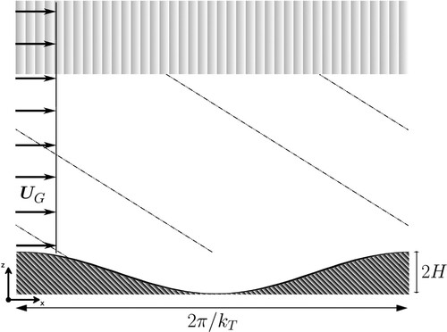
These values of $U_G$, N and of topography scales are typical of those encountered in the Southern Ocean, as discussed in Nikurashin and Ferrari (2010b) using measurements in the Drake passage and in the southeast Pacific region. For the Drake passage the latter authors showed that wave radiation is dominated by scales of 1 km and larger. This accounts for the value of 2 km (as in Nikurashin and Ferrari 2010a) and 1.2 km we consider.

2.2. Numerical set-up

The numerical simulations were carried out with Symphonie NH, a non-hydrostatic regional ocean model which solves the Navier-Stokes equations in the Boussinesq approximation (Auclair et al. 2011). The physical configuration involving a uniform flow over a y-invariant topography in a rotating reference frame, the velocity field is three-dimensional but all flow components depend upon the x- and z- coordinates only. Hence, the simulations are performed in a vertical $(x,z)$ plane. Periodic boundary conditions are used along the x-direction, consistent with the sinusoidal topography, and the wavelength of the topography is also the horizontal extent of the numerical domain, denoted L. The bottom boundary conditions are set either to free slip or to partial slip with a bottom roughness of 1 mm. To avoid wave reflection from the upper boundary, a damping layer of thickness 5000 m starting at 2000 m above the bottom is applied. Hence the height of the physical domain is 2000 m.

The flow is initiated from a state of rest. The horizontal velocity component is then forced through a body force $f{U}_G$ in the meridional momentum equation. During the first 24 h, the flow field is relaxed towards the desired value of $U_G$ with a time scale of 3 h, to damp spurious oscillations generated at the initial time. After 24 h, the relaxation is removed and the integration is carried out for 20 inertial periods.

The numerical grid has a fixed spacing in the horizontal direction equal to $\mathrm{\Delta }x=12.5$ m and a topography-following (σ-) coordinate along the vertical direction. In the damping layer, vertical grid spacing is stretched from about 5 m to about 300 m, and the viscosity and diffusivity are increased in proportion with the vertical grid spacing. The viscosity and diffusivity are set to ${10}^{-2}$ m${}^2$ s${}^{-1}$ and ${10}^{-3}$ m${}^2$ s${}^{-1}$, respectively, below the damping layer.

The numerical and physical parameters of the simulations are summarised in table 1. For clarity, the names of the calculations are composed of three parts: the height of the topography ($H_{20}$, $H_{40}$ or $H_{80}$); the horizontal length of the numerical domain, equal to either 2 km ($L_2$) or 1.2 km ($L_{1.2}$); the boundary condition, with either no mention if of the partial-slip type or denoted fs if of the free-slip type; and the Coriolis parameter, with either no mention if equal to the reference value of ${10}^{-4}$ s${}^{-1}$ or denoted $2f$ if equal to twice that value. (The generic Coriolis parameter and its reference value will therefore be designated by the same notation f for simplicity.)

Table 1. Summary of the simulations.

Simulation	L	H	f	Bottom condition	$U_G/NH$
$H_{20}{L}_2$	$2\mathrm{km}$	20 m	${1.10}^{-4}$ s${}^{-1}$	Partial-slip	5
$H_{40}{L}_2$	$2\mathrm{km}$	40 m	${1.10}^{-4}$ s${}^{-1}$	Partial-slip	2.5
$H_{80}{L}_2$	$2\mathrm{km}$	80 m	${1.10}^{-4}$ s${}^{-1}$	Partial-slip	1.25
$H_{20}{L}_2\mathrm{\_}fs$	$2\mathrm{km}$	20 m	${1.10}^{-4}$ s${}^{-1}$	Free-slip
$H_{40}{L}_2\mathrm{\_}fs$	$2\mathrm{km}$	40 m	${1.10}^{-4}$ s${}^{-1}$	Free-slip
$H_{80}{L}_2\mathrm{\_}fs$	$2\mathrm{km}$	80 m	${1.10}^{-4}$ s${}^{-1}$	Free-slip
$H_{20}{L}_{1.2}$	$1.2\mathrm{km}$	20 m	${1.10}^{-4}$ s${}^{-1}$	Partial-slip
$H_{40}{L}_{1.2}$	$1.2\mathrm{km}$	40 m	${1.10}^{-4}$ s${}^{-1}$	Partial-slip
$H_{80}{L}_{1.2}$	$1.2\mathrm{km}$	80 m	${1.10}^{-4}$ s${}^{-1}$	Partial-slip
$H_{40}{L}_2\mathrm{\_}2f$	$2\mathrm{km}$	40 m	${2.10}^{-4}$ s${}^{-1}$	Partial-slip
$H_{80}{L}_2\mathrm{\_}2f$	$2\mathrm{km}$	80 m	${2.10}^{-4}$ s${}^{-1}$	Partial-slip

Notes: L is the horizontal length of the numerical domain (equal to the horizontal wavelength of the topography), H is the half-height of the topography and f is the Coriolis parameter. Either partial-slip or free-slip boundary conditions are used at the topography for the velocity field. The other physical and numerical parameters are the same for all simulations and described in section 2.

2.3. Overall flow behaviour

In the following, as in Nikurashin and Ferrari (2010a), we decompose the flow into three components, which are the geostrophic flow, the IO field and the remaining internal gravity wave field. The IO velocity field is defined as: ${\mathit{U}}_{IO}(t,z)={\overline{\mathit{u}(x,z,t)-U_G}}^x$, where ${\overline{(.)}}^x$ denotes a horizontal average. This definition implies that (i) the IO horizontal scale is infinite (namely $k_{IO}=0$), (ii) the IO frequency is equal to f so the vertical group velocity vanishes, (iii) the IO field has no vertical velocity. The velocity field of the internal gravity wave field is defined as ${\mathit{U}}_{LW}(x,z,t)=\mathit{u}(x,z,t)-{\mathit{U}}_G-{\mathit{U}}_{IO}(t,z)$. This field has a zero horizontal average by definition and encompasses all motions that are not of zero horizontal wavenumber. At the beginning of the simulations, it coincides with the lee wave field of frequency $U_G{k}_T$ radiated by the geostrophic flow (in the frame of reference of that flow) and will be denoted in the following by the acronym LW for simplicity.

Over the range of parameters we consider, the topography is subcritical, namely the slope of the phase lines exceeds the slope of the topography. In the limit of long wavelength ($k_T\ll N/U_G$), the ratio of these two slopes is equal to $U_G/NH$, whose value is larger than 1 in the subcritical case. This parameter can also be interpreted as the ratio of the maximum distance a fluid particle can travel vertically, $U_G/N$, to the typical height of the topography, H. It follows that, when $U_G/NH>1$, the whole flow passes over the topography and no blocking occurs at the bottom of the topography. This is the case for all simulations we consider (see table 1).

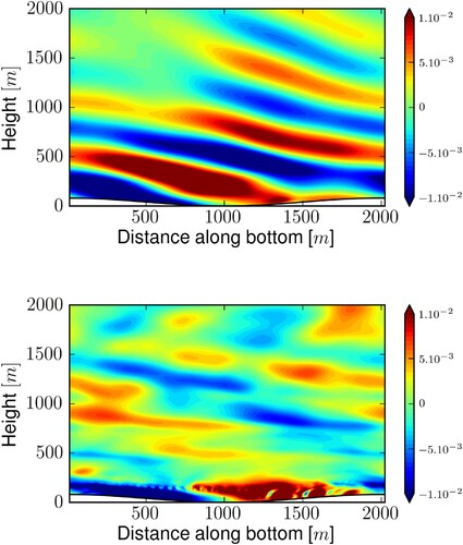
Basic features of the flow behaviour are illustrated in figure 2 for simulation $H_{40}{L}_2$ (see table 1). This figure displays the vertical velocity at two successive times. After one inertial period (upper frame), quasi-linear LW have been radiated and propagate upwards. After seven inertial periods (lower frame), wave breaking occurs at the bottom of the domain.

Figure 2. Snapshots of the vertical velocity for simulation $H_{40}{L}_2$ after one inertial period (upper frame) and after 7 inertial periods (lower frame). The same colorbar is used for the two frames, but the maximum value is about three times higher in the lower than in the upper frame. Note the quasi-linear regime in the upper frame and the strongly nonlinear regime in the lower one.

The amplitude of the IO field at a height of about 10 m above the topography top is displayed in figure 3 for all the simulations of table 1, except those with frequency $2f$ as explained below. The spin-up of the simulation, during which the mean flow grows from 0 to the value of $U_G$, is not shown. The IO amplitude is observed to grow, all the more so H or $k_T$ is larger. As shown in the next section, the IO growth rate is proportional to the square of the LW amplitude namely to $(H{k}_T{U}_G{)}^2$ (in the linear theory), which accounts qualitatively for the different growth rates observed. For H = 40 m and H = 80 m, a quasi-steady state is eventually reached in less than 10 inertial periods. For H = 20 m, the duration of the simulation is not long enough for the IO field to reach the quasi-steady state. Indeed, as discussed in section 4, the dissipation time scale based on the IO vertical wavelength is about 50 times the e-folding time of the IO growth implying that the latter growth is not damped (or only weakly so) by viscosity. Finally, for simulations with twice the inertial frequency f, the IO amplitude does not significantly depart from noise and is not shown.

Figure 3. Temporal evolution of the inertial oscillation (IO) amplitude at about 10 m above the topography top, as a function of time scaled by the inertial period $2\pi /f$. The IO signal was processed through a Lanczos low-pass filter at cutoff frequency f. The spin-up of the simulation, during which the geostrophic current grows from 0 to the value of $U_G$, is not shown (Colour online).

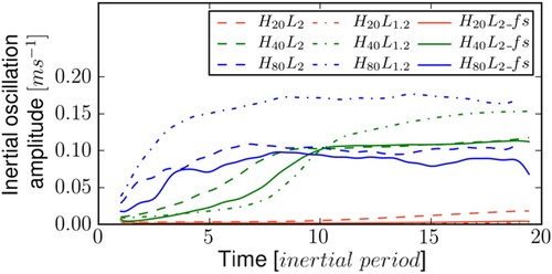
Figure 4 displays the vertical profile of the IO amplitude (upper frame) and of the TKE dissipation rate (lower frame) averaged from 12 to 15 inertial periods for all simulations in table 1 (except those with frequency $2f$). The upper frame shows that the IO amplitude has grown but remains localised close to the bottom of the domain, below 700 m or so. Consistent with the results displayed in figure 3, the maximum IO amplitude is all the larger the LW amplitude is higher. For H = 20 m, the IO amplitude remains insignificant throughout the water column. For $H\ge 40$ m, the maximum IO amplitude is of the same order as the geostrophic flow speed, ranging between about 1.1 and 2 times that speed. The lower frame of the figure shows that the TKE dissipation rate is most intense just above the topography, in the first 200 m or so, keeping significant values also below about 700 m.

Figure 4. Vertical structure of the IO horizontal velocity (upper frame) and of the horizontally-averaged TKE dissipation rate (lower frame) for the simulations displayed in table 1. All fields are averaged from 12 to 15 inertial periods (Colour online).

The next two sections aim at identifying the mechanisms at the origin of the IO growth and at quantifying their growth rate.

3. Resonant interactions involving internal lee waves and inertial oscillations

In the previous section, we have shown that IO emerge during the evolution of the flow. The objective of the present section is to show that IO can interact resonantly with LW within a wave triad. For this purpose, we rely on the resonant interaction theory (RIT) (see e.g. Phillips 1967).

We recall that LW are steady in the frame of reference attached to the topography, namely their absolute frequency vanishes. Since intrinsic wave frequencies are involved in the RIT, the theory is applied here in a frame of reference attached to the geostrophic flow $U_G$. In the following, the word frequency refers to this intrinsic frequency. We also recall that the RIT considers waves propagating in a vertical plane of infinite dimension in both directions, namely the presence of the topography is not taken into account.

3.1. Computation of the resonant triads

When three waves interact resonantly, significant energy exchanges can occur among these waves (compared to non resonant interactions) if the algebraic sum of both their wave vectors and their frequencies amount to zero. Assuming two of these waves are the LW and the IO and denoting the third wave with a $\ast$ subscript, these relations are expressed as (3a) $\begin{array}{rl}{\sigma }_{LW}{\mathit{k}}_{LW}+{\sigma }_{\ast }{\mathit{k}}_{\ast }+{\sigma }_{IO}{\mathit{k}}_{IO}& =0,\end{array}$(3a) (3b) $\begin{array}{rl}{\sigma }_{LW}{\omega }_{LW}+{\sigma }_{\ast }{\omega }_{\ast }+{\sigma }_{IO}{\omega }_{IO}& =0,\end{array}$(3b) where the subscripts refer to the different waves, $\sigma =\pm 1$, $\mathit{k}=(k,m)$ is the wave vector (in the present two-dimensional case) and ω the intrinsic frequency of either wave. We assume that all frequencies are positive implying that the σ coefficients cannot be of the same sign. Equations (3a(3a) $\begin{array}{rl}{\sigma }_{LW}{\mathit{k}}_{LW}+{\sigma }_{\ast }{\mathit{k}}_{\ast }+{\sigma }_{IO}{\mathit{k}}_{IO}& =0,\end{array}$(3a) ) and (3b(3b) $\begin{array}{rl}{\sigma }_{LW}{\omega }_{LW}+{\sigma }_{\ast }{\omega }_{\ast }+{\sigma }_{IO}{\omega }_{IO}& =0,\end{array}$(3b) ) together with the three dispersion relations yield 6 equations for 9 variables. Depending on the choice of $({\sigma }_{LW},{\sigma }_{\ast },{\sigma }_{IO})$, several triads can arise. We assume that the wave of largest amplitude is the internal lee wave. Since this wave has the same spectral properties throughout the different triads, the triads can be considered as independent (Chow et al. 1996).

The problem is closed by expressing that the LW parameters verify (4a) $\begin{array}{rl}{k}_{LW}& =k_T,\end{array}$(4a) (4b) $\begin{array}{rl}{\omega }_{LW}& =U_G{k}_T\end{array}$(4b) and by writing that the IO are homogeneous in the horizontal plane (5) $k_{IO}=0.$(5) We also know that ${\omega }_{IO}=f$ (or $|f|$ if f<0). The problem therefore boils down to 5 equations and 5 unknown variables ($m_{LW}$, $m_{IO}$, $k_{\ast }$, $m_{\ast }$, ${\omega }_{\ast }$) (6a) $\begin{array}{rl}{\sigma }_{LW}{k}_T+{\sigma }_{\ast }{k}_{\ast }& =0,\end{array}$(6a) (6b) $\begin{array}{rl}{\sigma }_{LW}{m}_{LW}+{\sigma }_{\ast }{m}_{\ast }+{\sigma }_{IO}{m}_{IO}& =0,\end{array}$(6b) (6c) $\begin{array}{rl}{\sigma }_{LW}{U}_G{k}_T+{\sigma }_{\ast }{\omega }_{\ast }+{\sigma }_{IO}f& =0,\end{array}$(6c) (6d) $\begin{array}{rl}{\omega }_{\ast }^2& =\frac{N^2{k}_{\ast }^2+f^2{m}_{\ast }^2}{k_{\ast }^2+m_{\ast }^2},\end{array}$(6d) (6e) $\begin{array}{rl}(U_G{k}_T{)}^2& =\frac{N^2{k}_T^2+f^2{m}_{LW}^2}{k_T^2+m_{LW}^2}.\end{array}$(6e) Solving these equations for the LW field yields (7a) $\begin{array}{rl}{k}_{LW}& =k_T,\end{array}$(7a) (7b) $\begin{array}{rl}{\omega }_{LW}& =U_G{k}_T,\end{array}$(7b) (7c) $\begin{array}{rl}{m}_{LW}& =-k_T\sqrt{\frac{N^2-(U_G{k}_T{)}^2}{(U_G{k}_T{)}^2-f^2}},\end{array}$(7c) where we chose $m_{LW}<0$ to ensure that the LW radiate energy away from topography.

To solve for the IO and the third wave fields, we first consider the case $-{\sigma }_{LW}={\sigma }_{IO}={\sigma }_{\ast }=1$. For the third wave of the triad, we obtain (8a) $\begin{array}{rl}{k}_{\ast }& =k_T,\end{array}$(8a) (8b) $\begin{array}{rl}{\omega }_{\ast }& =U_G{k}_T-f,\end{array}$(8b) (8c) $\begin{array}{rl}{m}_{\ast }& =\pm k_T\sqrt{\frac{N^2-(U_G{k}_T-f{)}^2}{(U_G{k}_T-f{)}^2-f^2}}.\end{array}$(8c) We recall that this internal wave can only exist provided $f<U_G{k}_T-f<N$. We notice from equation (8c(8c) $\begin{array}{rl}{m}_{\ast }& =\pm k_T\sqrt{\frac{N^2-(U_G{k}_T-f{)}^2}{(U_G{k}_T-f{)}^2-f^2}}.\end{array}$(8c) ) that the sign of $m_{\ast }$ is not determined implying that the $\ast$ wave can propagate either upwards or downwards. The vertical wavenumber of the IO is inferred from the relation $m_{IO}=m_{LW}-m_{\ast }$, implying that the spectral parameters of the IO are (9a) $\begin{array}{rl}{k}_{IO}& =0,\end{array}$(9a) (9b) $\begin{array}{rl}{\omega }_{IO}& =f,\end{array}$(9b) (9c) $\begin{array}{rl}{m}_{IO}& =-k_T(\sqrt{\frac{N^2-(U_G{k}_T{)}^2}{(U_G{k}_T{)}^2-f^2}}\pm \sqrt{\frac{N^2-(U_G{k}_T-f{)}^2}{(U_G{k}_T-f{)}^2-f^2}}).\end{array}$(9c) The case ${\sigma }_{LW}={\sigma }_{\ast }=-{\sigma }_{IO}=1$ is equivalent to the case described above.

Finally, the full solution for the case ${\sigma }_{LW}=-{\sigma }_{\ast }={\sigma }_{IO}=1$ is (10a) $\begin{array}{rl}{k}_{LW}& =k_T,\end{array}$(10a) (10b) $\begin{array}{rl}{\omega }_{LW}& =U_G{k}_T,\end{array}$(10b) (10c) $\begin{array}{rl}{m}_{LW}& =-\sqrt{\frac{N^2-(U_G{k}_T{)}^2}{(U_G{k}_T{)}^2-f^2}}{k}_T,\end{array}$(10c) (10d) $\begin{array}{rl}{k}_{\ast }& =k_T,\end{array}$(10d) (10e) $\begin{array}{rl}{\omega }_{\ast }& =U_G{k}_T+f,\end{array}$(10e) (10f) $\begin{array}{rl}{m}_{\ast }& =\pm \sqrt{\frac{N^2-(U_G{k}_T+f{)}^2}{(U_G{k}_T+f{)}^2-f^2}}{k}_T,\end{array}$(10f) (10g) $\begin{array}{rl}{k}_{IO}& =0,\end{array}$(10g) (10h) $\begin{array}{rl}{\omega }_{IO}& =f,\end{array}$(10h) (10i) $\begin{array}{rl}{m}_{IO}& =-k_T(\sqrt{\frac{N^2-(U_G{k}_T{)}^2}{(U_G{k}_T{)}^2-f^2}}\pm \sqrt{\frac{N^2-(U_G{k}_T+f{)}^2}{(U_G{k}_T+f{)}^2-f^2}}).\end{array}$(10i) In summary, two solutions arise for the frequency of the third wave (${\omega }_{\ast }=U_G{k}_T\pm f$), and for each solution two possibilities exist for the sign of the vertical wavenumber of the third wave ($m_{\ast }$), and hence for the value of $m_{IO}$. Therefore, there are four solutions for the vertical wavenumber of the IO.

These triads can in turn be involved in higher order interactions. For instance, the interaction between an IO of frequency f and a $\ast$ wave of frequency $U_G{k}_T-f$ may give rise to a new wave of frequency $U_G{k}_T-2f$. More generally, energy transfers occur along a discrete spectrum of frequencies $U_G{k}_T+nf$, where n is an integer (positive or negative) which must satisfy (11) $1-\frac{U_G{k}_T}{f}<n<\frac{N}{f}-\frac{U_G{k}_T}{f}$(11) expressing that these frequencies lie in the range of internal wave frequencies.

3.2. Evidence of resonant triads from spectral analysis

Figure 5 displays the frequency spectrum of the horizontal velocity component along the x-axis for the wave field for simulation $H_{20}{L}_2$. This wave field encompasses the IO and the internal gravity wave field (LW). The spectrum is computed in a frame of reference moving at speed $U_G$ since intrinsic frequencies are to be detected. The straight line is the confidence level at 99%, above which the spectrum significantly departs from red noise. Several peaks emerge from the power spectrum.

Figure 5. Variance preserving power spectrum of the horizontal velocity component of the wave field for simulation $H_{20}{L}_2$ computed at about 600 m above the bottom of the domain, in a frame of reference moving with the geostrophic velocity $U_G$. The wave field encompasses the entire flow, except for the geostrophic flow. The straight line is the confidence level at 99% implying that the spectrum significantly departs from red noise when it exceeds this line. The inertial and buoyancy frequencies and the frequencies predicted by the resonant interaction theory are indicated with a vertical dashed-dotted line. The length of the time series is 15 inertial periods implying that the spectral resolution is 0.01f.

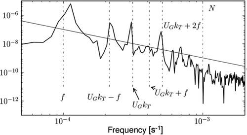
The peak close to f is that of the IO. This peak is indeed unchanged in the moving reference frame since the IO horizontal wavenumber vanishes. The peak is slightly shifted from (and above) f due to the finite length of the time series, equal to 15 inertial periods, and to nonlinear effects. Another peak is associated with the LW frequency ($\omega =U_G{k}_T$). One would expect the sum and difference of these two peaks ($\omega =U_G{k}_T\pm f$) to be dominant as well but only the difference of these frequencies appears, as explained in the next section. A peak at frequency $U_G{k}_T+2f$ also emerges but no peak of value $U_G{k}_T-2f$. No general conclusion about the presence of these peaks can be drawn however since, depending upon the simulation in table 1 we analysed, peaks at frequency $U_G{k}_T+3f$ or $U_G{k}_T+4f$ may instead (or also) be visible. But this clearly attests of the presence of higher order triads (which may be non resonant).

4. Growth rate of inertial oscillations

In this section we show that resonant interactions result in the growth of inertial oscillations. This growth rate is next compared with the one diagnosed from numerical simulations.

4.1. Expression of the inertial oscillation growth rate

Evolution equations for the amplitude of the waves involved in a resonant triad can be inferred from the RIT (see appendix A.1). This evolution occurs on a slow time scale, $t_1$ say (defined in that appendix). When one wave in the triad is of much larger amplitude than the other two (all waves being of very small amplitude, a basic assumption of the RIT), this large amplitude wave can be assumed to be steady over the time scale $t_1$. This allows for the linearisation of the evolution equations, from which the solution for the two smaller amplitude waves can be inferred. The latter waves either exchange energy within the triad over a periodic cycle, implying that their amplitude remains bounded, or their amplitude can grow exponentially, the largest amplitude wave feeding them. We consider the resonant triad made of the LW, assumed to have the largest amplitude, the IO and the * wave introduced in the previous section. In an inviscid fluid, the oscillatory or exponential behaviour depends upon the sign of the parameter ${\Gamma }^2$ defined by (12) ${\Gamma }^2={\left(\frac{A_{LW}}{2}\right)}^2{S}_{\ast }{S}_{IO},$(12) where $A_{LW}$ is the amplitude of the LW, and $S_{\ast }$ and $S_{IO}$ are interaction coefficients of the $\ast$ and IO waves, respectively, with the LW. The expression of these coefficients is (13a) $\begin{array}{rl}{S}_{\ast }& =\frac{{\sigma }_{LW}{\sigma }_{IO}}{2K_{\ast }^2{\omega }_{\ast }}[{\omega }_{\ast }(K_{LW}^2-K_{IO}^2)+N^2{k}_{\ast }(\frac{k_{LW]}}{{\omega }_{LW}}-\frac{k_{IO}}{{\omega }_{IO}})\\ & +f^2{m}_{\ast }(\frac{m_{LW}}{{\omega }_{LW}}LW-\frac{m_{IO}}{{\omega }_{IO}})](m_{IO}{k}_{LW}-m_{LW}{k}_{IO}),\end{array}$(13a) (13b) $\begin{array}{rl}{S}_{IO}& =\frac{{\sigma }_{LW}{\sigma }_{\ast }}{2K_{IO}^2{\omega }_{IO}}[{\omega }_{IO}(K_{LW}^2-K_{\ast }^2)+N^2{k}_{IO}(\frac{k_{LW}}{{\omega }_{LW}}-\frac{k_{\ast }}{{\omega }_{\ast }})\\ & +f^2{m}_{IO}(\frac{m_{LW}}{{\omega }_{LW}}-\frac{m_{\ast }}{{\omega }_{\ast }})](m_{\ast }{k}_{LW}-m_{LW}{k}_{\ast })\end{array}$(13b) with $K_i=|{\mathbf{k}}_{\mathbf{i}}\mathbf{|}$. When ${\Gamma }^2>0$, namely $S_{\ast }{S}_{IO}>0$, the IO and the * waves grow exponentially at rate Γ, implying that the LW is unstable in the inviscid limit. When ${\Gamma }^2<0$ ($S_{\ast }{S}_{IO}<0$), the LW is stable. The derivation of equation (12(12) ${\Gamma }^2={\left(\frac{A_{LW}}{2}\right)}^2{S}_{\ast }{S}_{IO},$(12) ) is detailed in appendix A.2, viscous and diffusive effects being taken into account.

4.2. Validation with numerical simulations

For the range of parameters considered in this paper, ${\Gamma }^2$ is strictly positive for the two triads involving the $\ast$ wave of frequency $U_G{k}_T-f$ (these triads differ by the value of $m_{IO}$). This result holds for all simulations except for those with twice the inertial frequency since $U_G{k}_T-2f<2f$ in this case. No resonant triad involving the LW and the IO can therefore be detected in the latter simulations.

The finding of these triads is consistent with Hasselman's criterion (Hasselmann 1967), which states that a primary wave is unstable if it has the highest frequency in the triad. Hence, the internal lee wave, of frequency $U_G{k}_T$, is unstable for a triad involving the IO and the $\ast$ wave at $U_G{k}_T-f$, but stable for a triad involving the IO and the $\ast$ wave at $U_G{k}_T+f$. (Hasselman's criterion can actually be shown to be equivalent to $S_{\ast }{S}_{IO}>0$.) In the former triad, energy is continuously transferred from the LW to the IO and the $\ast$ wave, whereas in the latter triad periodic energy exchange takes place between the three waves. This implies that although the two types of triads are expected to have a signature in the frequency spectrum displayed in figure 5, the triads involving the $\ast$ wave with frequency $U_G{k}_T-f$ should be dominant, which the latter figure attests.

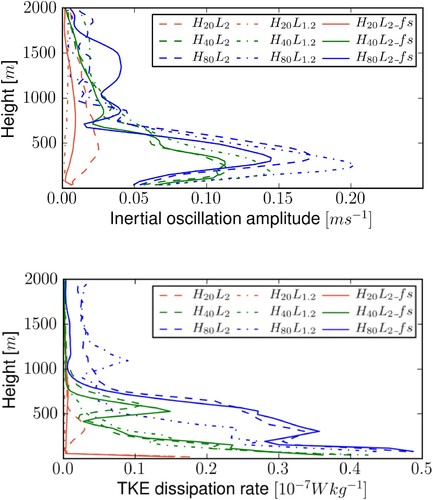
Figure 6 displays a scatter plot of Γ computed from the resonant interaction theory and from the simulations, denoted ${\Gamma }_{RIT}$ and ${\Gamma }_{sim}$, respectively (the expression of ${\Gamma }_{RIT}$ is derived in appendix A.2). The theory predicts growth rates of similar values when the sign of $m_{\ast }$ is changed (for instance, for H = 40 m, the value of ${\Gamma }_{RIT}/f$ is equal to $3.33{10}^{-1}$ for $m_{\ast }>0$ and to $3.76{10}^{-1}$ for $m_{\ast }<0$) and only the values associated with negative $m_{\ast }$ are shown for clarity. Also, values of ${\Gamma }_{RIT}$ in the inviscid limit are shown as the effect of viscosity hardly changes these values (see appendix A.2). Indeed the relative difference between the inviscid and the viscous values for ${\Gamma }_{RIT}$ are at most a few percents whatever H. As for the numerical growth rate ${\Gamma }_{sim}$, it is computed from an exponential fit of the curves displayed in figure 3 from the beginning of the simulations (namely, after the spin-up time). Only positive growth rates are shown.

Figure 6. Scatter diagram of the growth rate of the IO diagnosed from the simulations, ${\Gamma }_{sim}$, versus that computed from the resonant interaction theory, ${\Gamma }_{RIT}$, scaled by the inertial frequency. Simulations for which the inverse of the IO growth rate is smaller than 3 inertial periods are indicated with a filled marker (black or grey). For simulations with empty markers, the inverse of the IO growth rate is larger than 10 inertial periods.

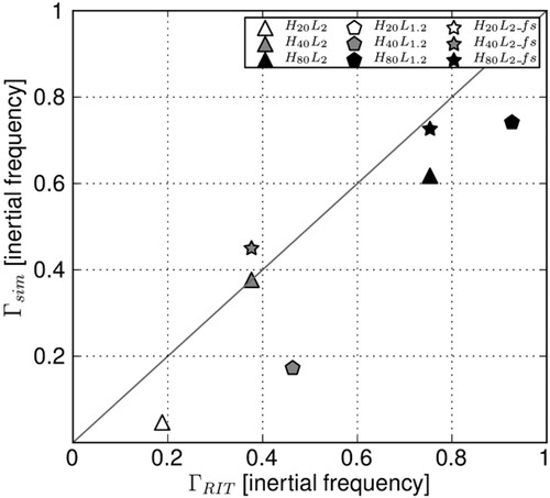
Since simulations with H = 20 m present little IO growth (see figure 3), a precise estimate of the growth rate for these simulations cannot be obtained, hence preventing the comparison with the theoretical predictions. The growth rates computed for cases with $H\ge 40$ are much more robust. For the latter cases, all values of ${\Gamma }_{sim}$ but one underestimate the theoretical predictions. More precisely, simulations with a free-slip boundary condition on the topography yield a growth rate in very good agreement with the theoretical predictions. This is no longer true when a half-slip boundary condition is used, consistent with the RIT being inviscid (the RIT predictions being hardly modified by viscous effects as said above). As well, when H = 80 m, higher order triads very likely interact with the dominant one, extracting energy from this triad and damping its growth rate. In overall, it can be concluded that the values of ${\Gamma }_{sim}$ agree reasonably well with those of ${\Gamma }_{RIT}$.

4.3. Vertical propagation of the inertial oscillations

As discussed in the previous section, we consider only the two triads involving the LW, the IO and the $\ast$ wave with frequency $U_G{k}_T-f$. These triads differ by the expression of the IO vertical wavenumber (14) $m_{IO}=-k_T(\sqrt{\frac{N^2-(U_G{k}_T{)}^2}{(U_G{k}_T{)}^2-f^2}}\pm \sqrt{\frac{N^2-(U_G{k}_T-f{)}^2}{(U_G{k}_T-f{)}^2-f^2}}),$(14) from where the expression of the IO phase speed in the vertical direction can be computed, $c_{\varphi }^z{|}_{IO}=f/m_{IO}$. The product $m_{\ast }{m}_{IO}$ is negative, meaning that a $\ast$ wave whose phase propagates downwards ($m_{\ast }<0$) is associated with an IO whose phase propagates upwards ($m_{IO}>0$).

Figure 7 displays a time-height diagram of the horizontal velocity of the IO for simulation $H_{20}{L}_2$. The value of the IO vertical phase speed predicted by the RIT for $m_{IO}>0$ is indicated with a black line. This value compares very well with the numerical result below about 1000 m, where the IO amplitude is the largest. As discussed above, a theoretical solution with a negative value of $m_{IO}$ is also found from RIT but it does not appear in the numerical solution. One possible explanation is that the latter IO wave is of smaller vertical scale than the $m_{IO}>0$ wave ($2\pi /|m_{IO}|$ is equal to 240 m for $m_{IO}<0$ and to 1015 m for $m_{IO}>0$) and therefore more prone to dissipation. Indeed, the viscous time scale (estimated as $1/(\nu m_{IO}^2)$) associated with the $m_{IO}<0$ wave is about 2 inertial periods, against 40 inertial periods for the $m_{IO}>0$ wave, which may account for the former wave to be of insignificant amplitude.

Figure 7. Time-height diagram of the IO horizontal velocity for $H_{20}{L}_2$. The slope of the black line is the vertical phase speed of the IO, $f/m_{IO}$, for the resonant triad involving a $\ast$ wave of frequency $U_G{k}_t-f$ and $m_{IO}>0$. The horizontal white line indicates the height of 1000 m (Colour online).

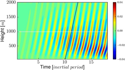
Figure 7 also shows that the IO field amplifies at lower heights with time, as if the IO were propagating energy downwards. This would imply that the IO is near-inertial. However, the formation of a near-inertial wave is forbidden by the periodic boundary conditions because these conditions quantify the horizontal wavenumbers into $n{k}_T$, with $n\ge 0$. A near-inertial oscillation would be associated with a non-zero and very small ($\ll k_T$) horizontal wavenumber, which is not possible. This behaviour of the IO field, possibly due to nonlinear effects, needs to be clarified.

5. Energy transfer from the lee waves to inertial oscillations versus TKE dissipation

The objective of this section is two-fold: (i) to estimate the energy transferred from the LW to the IO; (ii) to determine whether a relationship can be found between the IO kinetic energy and the TKE dissipation rate.

For this purpose, a scatter plot of the IO kinetic energy $E_{IO}$ and of the TKE dissipation rate ϵ is displayed in figure 8. Both quantities are integrated over the physical domain and averaged from 12 to 15 inertial periods, when the IO amplitude (see figure 3) and ϵ (see Labreuche 2015, figure 2.3) have reached a quasi-steady regime. The quantity ϵ is scaled with the LW energy flux $p^{\prime }w$ taken at about 10 m above the top of the topography and averaged horizontally over the physical domain, denoted $P_{up}$ ($p^{\prime }$ is the pressure deviation from hydrostatic balance). The quantity $E_{IO}$ is scaled by the LW energy flux during one inertial period $P_{up}/(2\pi /f)$.

Figure 8. Scatter plot of the IO kinetic energy $E_{IO}$ versus the TKE dissipation rate ϵ integrated over the physical domain D and from 12 to 15 inertial periods. ϵ is scaled by the LW energy flux taken at a height of about 10 m above the topography top and averaged horizontally over the physical domain, denoted $P_{up}$. The IO kinetic energy is scaled by $P_{up}$ during one inertial period $2\pi /f$. Simulations for which the inverse of the IO growth rate is smaller than 3 inertial periods are indicated with a filled marker (black or grey). For simulations with empty markers, the inverse of the IO growth rate is larger than 10 inertial periods. The + and × signs refer to simulations with Coriolis frequency $2f$, for which ${\Gamma }^2<0$.

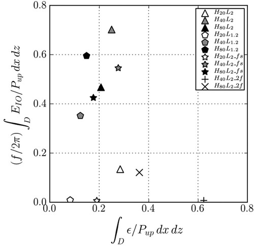
Figure 8 shows that, for H larger than 40 m and $f={10}^{-4}{\mathrm{s}}^{-1}$, an appreciable part of the energy transported by the LW over one inertial period is converted to IO kinetic energy, comprised between 35% and 70%. For H = 20 m, the growth rate of the IO is very small ($1/\Gamma$ is greater that 10 inertial periods) and $E_{IO}$ does not exceed 15% of the LW energy flux during one inertial period, being vanishingly small when the domain size is 1.2 km or if a free-slip boundary condition is used. For f twice larger, ${\Gamma }^2$ defined by equation (12(12) ${\Gamma }^2={\left(\frac{A_{LW}}{2}\right)}^2{S}_{\ast }{S}_{IO},$(12) ) is negative and no IO can grow by resonant interactions. This is attested in the figure (+ symbol) for H = 40 m. For H = 80 m, IO kinetic energy is still detected (× symbol), the IO field having possibly been created by nonlinear (non-resonant) interactions during the turbulent regime; however their kinetic energy is not more than 12% of the LW energy flux during one inertial period. In overall, figure 8 shows that resonant interactions are an efficient mechanism to force IO from the LW.

Focusing now on the total TKE dissipation rate, figure 8 shows that ϵ is comprised between about 10 and 30% of the LW energy flux for $f={10}^{-4}{\mathrm{s}}^{-1}$ (when IO grow). These values are consistent with ratios of dissipated to radiated energy (estimated from wave radiation theory) observed in the Scotia Sea within 1 km of the seabed (Sheen et al. 2013). Figure 8 also shows that ϵ is largest when ${\Gamma }^2<0$, namely when no resonant growth of IO occurs (see the simulations with frequency $2f$). It follows from this figure that no clear dependence of the total TKE dissipation rate upon the total IO kinetic energy can be inferred, even though the vertical structure of the IO and of ϵ seems to be related (see figure 4). Therefore, for the set of parameters we consider, it is not possible to infer the TKE dissipation rate from the IO amplitude.

6. Conclusion and discussion

The interactions between lee waves (LW) and inertial oscillations (IO) are addressed in this paper for an idealised configuration and a range of parameters typical of the Southern Ocean. The lee waves are radiated by a geostrophic flow over a two-dimensional sinusoidal topography in a stably-stratified fluid of constant buoyancy frequency N at mid-latitude. Inertial oscillations are internal gravity waves of frequency equal to the Coriolis frequency f (assumed positive for simplicity). The main result of this paper is that IO can grow by triadic resonant interactions with the LW. The dominant triad involves waves with frequency $U_G{k}_T$, f and $U_G{k}_T-f$, where $U_G{k}_T$ is the intrinsic frequency of the LW (measured in a frame of reference attached to the geostrophic flow of speed $U_G$; $k_T$ is the horizontal wavenumber of the topography). This resonant mechanism is valid whatever the parameters of the problem provided the LW intrinsic frequency is comprised between $2f$ (as $U_G{k}_T-f$ should be larger than f) and N. For $f={10}^{-4}$, $N={10}^{-3}$ and $U_G=0.1\mathrm{m}{\mathrm{s}}^{-1}$, which are the values considered in the present configurations, this condition implies that the wavelength of the topography is comprised between 600 m and 3 km, which are typical values for oceanic bottom topographies.

The resonant growth mechanism of IO is assessed from numerical simulations with wavelength of the topography equal to 1.2 km and 2 km. IO do grow in the simulations, in a bottom layer of height less than 1000 m, with a growth rate in good agreement with predictions of inviscid resonant interaction theory (RIT). This theory predicts that two resonant triads can occur, associated with IO with either a positive (upward) or a negative (downward) phase speed along the vertical direction. Only the former triad is found in the simulations consistent with oceanic observations (e.g. Leaman and Sanford 1975). A possible argument to account for the absence of the negative phase speed IO is that the latter wave is damped by viscosity.

IO have a zero group velocity so they amplify at their generation site. This is close to the bottom in the present case, possibly because the LW away from the topography are no longer energetic enough to amplify the IO (having forced them close to the bottom), dispersive and viscous effects coming also into play. We remind that, for internal gravity waves, a positive phase speed along the vertical is associated with a negative vertical group velocity. Thus, in the ocean where near-inertial oscillations can be generated, these results imply that the latter waves should accumulate close to the topography while growing, possibly leading to mixing via shear instability. Such a downward energy propagation of near-inertial oscillations close to rough bathymetry has been observed, e.g. by Alford (2010) in the Eastern North Pacific and by Waterman et al. (2014) in the Southern Ocean. In the latter case, measurements show an elevated energy dissipation rate up to $\simeq 250$ m above the topography (see Zemskova and Grisouard 2021, for further references and discussion).

In the present paper, the amplitude evolves in time toward a quasi-steady regime, reaching values as large as the speed of the geostrophic flow when the parameter $U_G/NH$ is order 1 (H is the half-height of the topography). During this regime, depending upon the flow parameters, the IO kinetic energy is equal to 30–70 % of the LW energy flux during one inertial period. This wide range of variation is not reflected in the TKE dissipation rate: this rate is comprised between 10 and 30% of the LW energy flux, whatever the IO amplitude, even if vanishingly small. Therefore, for the set of parameters we consider, it cannot be concluded that the TKE dissipation rate can be inferred from the IO amplitude.

The RIT framework considered in this paper is no longer valid during the quasi-steady regime, LW being now radiated by the superposition of the geostrophic flow and the IO field of similar amplitude. This flow regime is studied by Nikurashin and Ferrari (2010a). An asymptotic expansion as a function of the LW amplitude is derived by these authors, in which the geostrophic flow and the IO are zero order fields. It is shown that the IO are forced by the divergence of the wave-induced Reynolds stress, this divergence being due to dissipative effects. Dissipation is introduced in the equations of motion by a Rayleigh damping force to make the problem mathematically tractable. This forcing mechanism of the IO therefore requires very different assumptions than the one proposed in the present paper: in the RIT, the IO amplitude is much smaller that the LW amplitude and dissipative effects do not play any role. These two mechanisms can actually be seen as complementary: infinitely small amplitude IO grow by inviscid resonant interactions involving the LW and when the IO amplitude becomes of the same order as that of the geostrophic flow, momentum deposition by the LW comes into play through a viscous nonlinear process, which forces the IO.

The results presented in this paper have actually more generality, as literature on the internal tide shows it. Indeed Nikurashin and Legg (2011), while adressing the mechanism of turbulent energy dissipation above the bottom in the Brazil basin from the internal tide, found from two-dimensional numerical simulations that the triad (${\omega }_{tide},f,{\omega }_{tide}-f$) is dominant in the energy spectrum in the first 1000 m above the bottom (${\omega }_{tide}$ denotes the tidal frequency). These authors conclude that this triad is a key player in energy transfer from the internal tide to small vertical scale waves and therefore in turbulent processes. Richet et al. (2018) showed that this triad is a resonant triad, similarly to the present finding where the energy source is provided by the lee waves. From the work of Richet et al. (2018), one can actually note that, as f increases from 0 at the equator to its value at the critical latitude defined by $f_c={\omega }_{tide}/2$, the frequency of the secondary waves f and ${\omega }_{tide}-f$ becomes each equal to ${\omega }_{tide}/2$, namely the resonant process becomes of the parametric subharmonic instability type. This points toward the crucial role of this resonant triad as f varies from 0 to $f_c$ and of IO in energy transfer toward small scales in the ocean.

These results imply that IO should be taken into account in the parameterisation of mixing in the ocean (as also stressed by Alford et al. 2016). Indeed, it is usually assumed in such parameterizations that the turbulent cascade is driven by wave-wave interactions not subject to rotation. The present paper shows that the nonlinear interaction between lee waves and IO is critical to setting the energy spectrum.

Acknowledgments

The authors thank Matthieu Leclair and Francis Auclair for technical assistance with the model configuration. Symbolic calculations were performed with SageMath (Stein 2012). We are grateful to Maxim Nikurashin and Jacques Vanneste for fruitful discussions. Computations were performed on the CINES supercomputer centre. The authors received funding from the Laboratoire d'Excellence OSUG@2020 and from the national Program LEFE of the INSU-CNRS.

Disclosure statement

No potential conflict of interest was reported by the author(s).

Notes

1 The critical latitude is the latitude at which the Coriolis parameter is half the tidal frequency.

Appendix: Resonant interaction theory

This annex is a step by step guide through the resonant interaction theory derivation.

A.1. Derivation of the amplitude equations

Let $(u,v,w)$ be the velocity components of the internal gravity wave field. In the paper, these components do not depend upon the y-coordinate so that a stream function ψ can be introduced: $u=-\mathrm{\partial }\psi /\mathrm{\partial }z$, $w=\mathrm{\partial }\psi /\mathrm{\partial }x$. We note the density deviation with respect to hydrostatic balance as ρ. The Navier-Stokes equations in the Boussinesq approximation can thus be written as (e.g. Koudella and Staquet 2006) (A.1a) $\begin{array}{rl}{\mathrm{\partial }}_t\mathrm{\Delta }\psi +J(\omega ,\psi )& =f{\mathrm{\partial }}_{z}v+{\mathrm{\partial }}_x\rho +\nu {\mathrm{\Delta }}^2\psi ,\end{array}$(A.1a) (A.1b) $\begin{array}{rl}{\mathrm{\partial }}_{t}v+J(v,\psi )& =-f{\mathrm{\partial }}_z\psi +\nu \mathrm{\Delta }v,\end{array}$(A.1b) (A.1c) $\begin{array}{rl}{\mathrm{\partial }}_t\rho +J(\rho ,\psi )& =-N^2{\mathrm{\partial }}_x\psi +\kappa \mathrm{\Delta }\rho ,\end{array}$(A.1c) where ν is the molecular viscosity and κ the diffusivity of buoyancy.

These equations are scaled using $N^{-1}$ as a time scale, 1/K as a length scale with K being a typical wavenumber of the wave field and U as a velocity scale of the fluid particles displaced by the waves. Introducing the Froude number $Fr=UK/N$, the scaled equations become (keeping the same notation for the original and scaled variables) (A.2a) $\begin{array}{rl}{\mathrm{\partial }}_t\mathrm{\Delta }\psi +FrJ(\mathrm{\Delta }\psi ,\psi )& =\frac{f}{N}{\mathrm{\partial }}_{z}v+{\mathrm{\partial }}_x\rho +\frac{Fr}{Re}{\mathrm{\Delta }}^2\psi ,\end{array}$(A.2a) (A.2b) $\begin{array}{rl}{\mathrm{\partial }}_{t}v+FrJ(v,\psi )& =-\frac{f}{N}{\mathrm{\partial }}_z\psi +\frac{Fr}{Re}\nu \mathrm{\Delta }v,\end{array}$(A.2b) (A.2c) $\begin{array}{rl}{\mathrm{\partial }}_t\rho +FrJ(\rho ,\psi )& =-{\mathrm{\partial }}_x\psi .+\frac{Fr}{RePr}\mathrm{\Delta }\rho .\end{array}$(A.2c) $Re=U/\nu K$ and $Pr=\nu /\kappa$ are the Reynolds and Prandtl number, respectively.

Assuming that the Froude number is much smaller than 1, we introduce a fast-time scale $t_0$, of order $N^{-1}$, and a slow-time scale $t_1=Fr{t}_0$ over which resonant interactions take place: $t=t_0+Fr{t}_1$. Thus (A.3a) $\begin{array}{rl}{\mathrm{\partial }}_t& ={\mathrm{\partial }}_{t_0}+Fr{\mathrm{\partial }}_{t_1},\end{array}$(A.3a) (A.3b) $\begin{array}{rl}{\mathrm{\partial }}_t^2& ={\mathrm{\partial }}_{t_0}^2+2Fr{\mathrm{\partial }}_{t_0}{\mathrm{\partial }}_{t_1}+F{r}^2{\mathrm{\partial }}_{t_1}^2.\end{array}$(A.3b) We then expand the fields as a function of the small parameter Fr (A.4a) $\begin{array}{rl}\psi (\mathit{x},t_0,t_1)& ={\psi }^0(\mathit{x},t_0,t_1)+Fr{\psi }^1(\mathit{x},t_0,t_1)+\mathrm{O}(F{r}^2),\end{array}$(A.4a) (A.4b) $\begin{array}{rl}v(\mathit{x},t_0,t_1)& =v^0(\mathit{x},t_0,t_1)+Fr{v}^1(\mathit{x},t_0,t_1)+\mathrm{O}(F{r}^2),\end{array}$(A.4b) (A.4c) $\begin{array}{rl}\rho (\mathit{x},t_0,t_1)& ={\rho }^0(\mathit{x},t_0,t_1)+Fr{\rho }^1(\mathit{x},t_0,t_1)+\mathrm{O}(F{r}^2).\end{array}$(A.4c) At zero order, assuming that the fields are not damped by viscosity, one obtains (A.5a) $\begin{array}{rl}{\mathrm{\partial }}_{t_0}^2\mathrm{\Delta }{\psi }^0+{\psi }_{xx}^0+{\left(\frac{f}{N}\right)}^2{\psi }_{zz}^0& =0,\end{array}$(A.5a) (A.5b) $\begin{array}{rl}{\mathrm{\partial }}_{t_0}{v}^0+\frac{f}{N}{\mathrm{\partial }}_z{\psi }^0& =0,\end{array}$(A.5b) (A.5c) $\begin{array}{rl}{\mathrm{\partial }}_{t_0}{\rho }^0+{\psi }_x^0& =0.\end{array}$(A.5c) Thus, the solution at zero-order describes the evolution of plane waves. We assume that these plane waves consist in the superposition of three waves whose amplitude varies slowly in time (A.6a) $\begin{array}{rl}{\psi }^0(\mathit{x},t_0,t_1)& =\sum _{j=0}^2{A}_i(t_1){\mathrm{e}}^{\mathrm{i}{\varphi }_i}+\text{c.c.},\end{array}$(A.6a) (A.6b) $\begin{array}{rl}{v}^0(\mathit{x},t_0,t_1)& =\sum _{j=0}^2\frac{f}{N}\frac{m_i}{{\omega }_i}{A}_i(t_1){\mathrm{e}}^{\mathrm{i}{\varphi }_i}+\text{c.c.},\end{array}$(A.6b) (A.6c) $\begin{array}{rl}{\rho }^0(\mathit{x},t_0,t_1)& =\sum _{j=0}^2\frac{k_i}{{\omega }_i}{A}_i(t_1){\mathrm{e}}^{\mathrm{i}{\varphi }_i}+\text{c.c.},\end{array}$(A.6c) where ${\varphi }_j$ is the phase of the j-wave ${\varphi }_j={\mathit{k}}_{\mathit{j}}\mathbf{.}\mathit{x}-{\omega }_j{t}_0\mathrm{with}{\mathit{k}}_{\mathit{j}}=(k_j,m_j).$ At order 1, viscous and diffusive effects are taken into account. Careful development of that order leads to (A.7) $\sum _{{\sigma }_l=\pm 1}\sum _{l=0}^2{\mathcal{F}}_l+\sum _{{\sigma }_n=\pm 1}\sum _{{\sigma }_p=\pm 1}\sum _{n=0}^2\sum _{p=0}^2{\mathcal{G}}_{n,p}=0,$(A.7) where ${\mathcal{F}}_l$ gathers the linear terms and ${\mathcal{G}}_{n,p}$ the non-linear terms (A.8) $\begin{array}{rl}{\mathcal{F}}_l=& -\mathrm{i}{\sigma }_l{K}_l^2{\omega }_l{\mathrm{e}}^{\mathrm{i}{\sigma }_l{\varphi }_l}[2\frac{\mathrm{\partial }{A}_l^{({\sigma }_l)}}{\mathrm{\partial }{t}_1}+\frac{1}{RePr}\frac{k_l^2}{{\omega }_l^2}{A}_l^{({\sigma }_l)}+\frac{1}{Re}{K}_l^2{A}_l^{({\sigma }_l)}-{\left(\frac{f}{N}\right)}^2\frac{1}{Re}\frac{m_l^2}{{\omega }_l^2}{A}_l^{({\sigma }_l)}],\end{array}$(A.8) (A.9) $\begin{array}{rl}{\mathcal{G}}_{n,p}& =\mathrm{i}{\sigma }_n{\sigma }_p(m_n{k}_p-m_p{k}_n)A_n^{({\sigma }_n)}{A}_p^{({\sigma }_p)}{\mathrm{e}}^{\mathrm{i}({\sigma }_n{\varphi }_n+{\sigma }_p{\varphi }_p)}\\ & \times [K_p^2({\sigma }_n{\omega }_n+{\sigma }_p{\omega }_p)+\frac{k_p}{{\omega }_p}({\sigma }_n{k}_n+{\sigma }_p{k}_p)+{\left(\frac{f}{N}\right)}^2\frac{m_p}{{\omega }_p}({\sigma }_n{m}_n+{\sigma }_p{m}_p)],\end{array}$(A.9) where $A_j^{(1)}=A_j$ and $A_j^{(-1)}$ is the complex conjugate.

Taking into account that $K_j^2{\omega }_j-(f/N{)}^2{m}_j^2/{\omega }_j=k_j^2/{\omega }_j$ from the dispersion relation, the equations become (A.10) $\begin{array}{rl}& \sum _{{\sigma }_l=\pm 1}\sum _l{\mathrm{e}}^{\mathrm{i}{\sigma }_l{\varphi }_l}\left[{\sigma }_l{K}_l^2{\omega }_l(2\frac{\mathrm{\partial }{A}_l^{({\sigma }_l)}}{\mathrm{\partial }{t}_1}+\frac{1}{Re}\frac{k_l^2}{{\omega }_l^2}(1+\frac{1}{Pr})A_l^{({\sigma }_l)})\right]\\ & =\sum _{\begin{array}{c}{\sigma }_n=\pm 1\\ {\sigma }_p=\pm 1\end{array}}\sum _{n,p}{\mathrm{e}}^{\mathrm{i}({\sigma }_n{\varphi }_n+{\sigma }_p{\varphi }_p)}[{\sigma }_n{\sigma }_p(m_n{k}_p-m_p{k}_n)A_n^{({\sigma }_n)}{A}_p^{({\sigma }_p)}\phantom{{\left(\frac{f}{N}\right)}^2}\\ & \times (K_p^2({\sigma }_n{\omega }_n+{\sigma }_p{\omega }_p)+\frac{k_p}{{\omega }_p}({\sigma }_n{k}_n+{\sigma }_p{k}_p)+{\left(\frac{f}{N}\right)}^2\frac{m_p}{{\omega }_p}({\sigma }_n{m}_n+{\sigma }_p{m}_p))].\end{array}$(A.10) From this equation, it follows that for resonant interaction to occur, the waves need to satisfy (A.11) $\mathrm{\forall }\{l,n,p\}\in \{0,1,2{\}}^3,l\ne n\ne p,\mathrm{\exists }({\sigma }_l,{\sigma }_n,{\sigma }_p)\in \{-1,1{\}}^3,{\sigma }_l{\varphi }_l={\sigma }_n{\varphi }_n+{\sigma }_p{\varphi }_p.$(A.11) We can here choose the convention ${\omega }_j>0$ without any loss of information. The resonant condition can be written as $\mathrm{\forall }\{l,n,p\}\in \{0,1,2{\}}^3,l\ne n\ne p,\mathrm{\exists }({\sigma }_l,{\sigma }_n,{\sigma }_p)\in \{-1,1{\}}^3,$ (A.12a) $\begin{array}{rl}{\sigma }_l{\omega }_l& ={\sigma }_n{\omega }_n+{\sigma }_p{\omega }_p,\end{array}$(A.12a) (A.12b) $\begin{array}{rl}{\sigma }_l{\mathit{k}}_l& ={\sigma }_n{\mathit{k}}_n+{\sigma }_p{\mathit{k}}_p.\end{array}$(A.12b) Injecting the resonant condition into (A.10(A.10) $\begin{array}{rl}& \sum _{{\sigma }_l=\pm 1}\sum _l{\mathrm{e}}^{\mathrm{i}{\sigma }_l{\varphi }_l}\left[{\sigma }_l{K}_l^2{\omega }_l(2\frac{\mathrm{\partial }{A}_l^{({\sigma }_l)}}{\mathrm{\partial }{t}_1}+\frac{1}{Re}\frac{k_l^2}{{\omega }_l^2}(1+\frac{1}{Pr})A_l^{({\sigma }_l)})\right]\\ & =\sum _{\begin{array}{c}{\sigma }_n=\pm 1\\ {\sigma }_p=\pm 1\end{array}}\sum _{n,p}{\mathrm{e}}^{\mathrm{i}({\sigma }_n{\varphi }_n+{\sigma }_p{\varphi }_p)}[{\sigma }_n{\sigma }_p(m_n{k}_p-m_p{k}_n)A_n^{({\sigma }_n)}{A}_p^{({\sigma }_p)}\phantom{{\left(\frac{f}{N}\right)}^2}\\ & \times (K_p^2({\sigma }_n{\omega }_n+{\sigma }_p{\omega }_p)+\frac{k_p}{{\omega }_p}({\sigma }_n{k}_n+{\sigma }_p{k}_p)+{\left(\frac{f}{N}\right)}^2\frac{m_p}{{\omega }_p}({\sigma }_n{m}_n+{\sigma }_p{m}_p))].\end{array}$(A.10) ) yields (A.13) $\begin{array}{rl}\frac{\mathrm{\partial }{A}_l^{({\sigma }_l)}}{\mathrm{\partial }{t}_1}+\frac{1}{Re}\frac{k_l^2}{2{\omega }_l^2}& (1+\frac{1}{Pr})A_l^{({\sigma }_l)}={\sigma }_n{\sigma }_p{A}_n^{({\sigma }_n)}{A}_p^{({\sigma }_p)}\frac{(m_n{k}_p-m_p{k}_n)}{2K_l^2{\omega }_l}\\ & \times [(K_p^2-K_n^2){\omega }_l+(\frac{k_p}{{\omega }_p}-\frac{k_n}{{\omega }_n})k_l+{\left(\frac{f}{N}\right)}^2(\frac{m_p}{{\omega }_p}-\frac{m_n}{{\omega }_n})m_l].\end{array}$(A.13) Let us rewrite the two main results from this section in a more general way (in equations (A.12(A.12a) $\begin{array}{rl}{\sigma }_l{\omega }_l& ={\sigma }_n{\omega }_n+{\sigma }_p{\omega }_p,\end{array}$(A.12a) ) ${\sigma }_l$ is changed into $-{\sigma }_l$, without any loss of generality) (A.14a) $\begin{array}{rl}{\sigma }_l{\omega }_l+{\sigma }_n{\omega }_n+{\sigma }_p{\omega }_p& =0,\end{array}$(A.14a) (A.14b) $\begin{array}{rl}{\sigma }_l{\mathit{k}}_l+{\sigma }_n{\mathit{k}}_n+{\sigma }_p{\mathit{k}}_p& =0.\end{array}$(A.14b) The final amplitude evolution equation becomes (A.15) $\begin{array}{rl}\frac{\mathrm{\partial }{A}_l^{({\sigma }_l)}}{\mathrm{\partial }{t}_1}+\frac{1}{Re}\frac{k_l^2}{2{\omega }_l^2}& (1+\frac{1}{Pr})A_l^{({\sigma }_l)}={\sigma }_n{\sigma }_p{A}_n^{(-{\sigma }_n)}{A}_p^{(-{\sigma }_p)}\frac{(m_n{k}_p-m_p{k}_n)}{2K_l^2{\omega }_l}\\ & \times [(K_p^2-K_n^2){\omega }_l+(\frac{k_p}{{\omega }_p}-\frac{k_n}{{\omega }_n})k_l+{\left(\frac{f}{N}\right)}^2(\frac{m_p}{{\omega }_p}-\frac{m_n}{{\omega }_n})m_l].\end{array}$(A.15)

A.2. Calculation of the growth rate

Let us assume that wave 0 is originally of large amplitude (this is the ILW in the present paper), and serves as thermostat to the system (it provides energy, and its amplitude is subject to only small relative variations on timescale $t_1$). Waves 1 and 2 are originally of small amplitude, and grow thanks to the energy provided by wave 0.

From equation (A.15(A.15) $\begin{array}{rl}\frac{\mathrm{\partial }{A}_l^{({\sigma }_l)}}{\mathrm{\partial }{t}_1}+\frac{1}{Re}\frac{k_l^2}{2{\omega }_l^2}& (1+\frac{1}{Pr})A_l^{({\sigma }_l)}={\sigma }_n{\sigma }_p{A}_n^{(-{\sigma }_n)}{A}_p^{(-{\sigma }_p)}\frac{(m_n{k}_p-m_p{k}_n)}{2K_l^2{\omega }_l}\\ & \times [(K_p^2-K_n^2){\omega }_l+(\frac{k_p}{{\omega }_p}-\frac{k_n}{{\omega }_n})k_l+{\left(\frac{f}{N}\right)}^2(\frac{m_p}{{\omega }_p}-\frac{m_n}{{\omega }_n})m_l].\end{array}$(A.15) ), the set of amplitude evolution equations becomes (A.16a) $\begin{array}{rl}{\mathrm{\partial }}_{t_1}{A}_1^{({\sigma }_1)}+C_1{A}_1^{({\sigma }_1)}& =S_1{A}_0^{(-{\sigma }_0)}{A}_2^{(-{\sigma }_2)},\end{array}$(A.16a) (A.16b) $\begin{array}{rl}{\mathrm{\partial }}_{t_1}{A}_2^{({\sigma }_2)}+C_2{A}_2^{({\sigma }_2)}& =S_2{A}_0^{(-{\sigma }_0)}{A}_1^{(-{\sigma }_1)},\end{array}$(A.16b) where (A.17a) $\begin{array}{rl}{C}_i=& \frac{1}{Re}\frac{k_i^2}{2{\omega }_i^2}(1+\frac{1}{Pr}),\end{array}$(A.17a) (A.17b) $\begin{array}{rl}{S}_1=& {\sigma }_0{\sigma }_2\frac{(m_2{k}_0-m_0{k}_2)}{2K_1^2{\omega }_1}\\ & \times [(K_0^2-K_2^2){\omega }_1+(\frac{k_0}{{\omega }_0}-\frac{k_2}{{\omega }_2})k_1+{\left(\frac{f}{N}\right)}^2(\frac{m_0}{{\omega }_0}-\frac{m_2}{{\omega }_2})m_1],\end{array}$(A.17b) (A.17c) $\begin{array}{rl}{S}_2=& {\sigma }_0{\sigma }_1\frac{(m_1{k}_0-m_0{k}_1)}{2K_2^2{\omega }_2}\\ & \times [(K_0^2-K_1^2){\omega }_2+(\frac{k_0}{{\omega }_0}-\frac{k_1}{{\omega }_1})k_2+{\left(\frac{f}{N}\right)}^2(\frac{m_0}{{\omega }_0}-\frac{m_1}{{\omega }_1})m_2].\end{array}$(A.17c) Since $(C_1,C_2,S_1,S_2)\in {\mathbb{R}}^4$, we can rewrite equation (A.16a(A.16a) $\begin{array}{rl}{\mathrm{\partial }}_{t_1}{A}_1^{({\sigma }_1)}+C_1{A}_1^{({\sigma }_1)}& =S_1{A}_0^{(-{\sigma }_0)}{A}_2^{(-{\sigma }_2)},\end{array}$(A.16a) ) as (A.18a) $\begin{array}{rl}({\mathrm{\partial }}_{t_1}+C_2)({\mathrm{\partial }}_{t_1}+C_1)A_1& =S_1{S}_2|A_0{|}^2{A}_1,\end{array}$(A.18a) (A.18b) $\begin{array}{rl}({\mathrm{\partial }}_{t_1}+C_2)({\mathrm{\partial }}_{t_1}+C_1)A_2& =S_1{S}_2|A_0{|}^2{A}_2.\end{array}$(A.18b) We can already deduce from equation (A.18a(A.18a) $\begin{array}{rl}({\mathrm{\partial }}_{t_1}+C_2)({\mathrm{\partial }}_{t_1}+C_1)A_1& =S_1{S}_2|A_0{|}^2{A}_1,\end{array}$(A.18a) ) that waves 1 and 2 will have the same time evolution.

Let $A_1(t_1)=A_1(0){\mathrm{e}}^{\Gamma t_1}$ and $A_2(t_1)=A_2(0){\mathrm{e}}^{\Gamma t_1}$, where Γ is the growth rate of the secondary waves. This entails (A.19) ${\Gamma }^2+(C_1+C_2)\Gamma +C_1{C}_2-S_1{S}_2|A_0{|}^2=0.$(A.19) The secondary waves will grow if Γ is real and positive, which occurs if (A.20) ${\mathrm{\Delta }}_{\Gamma }=(C_1+C_2{)}^2-4(C_1{C}_2-S_1{S}_2|A_0{|}^2)>0.$(A.20) If this is the case, the exponential growth rate of the waves is (A.21) $\Gamma =\frac{1}{2}[-(C_1+C_2)+\sqrt{(C_1-C_2{)}^2+4S_1{S}_2|A_0{|}^2}].$(A.21) Viscosity damps the growth rate as expected.

References

- Alford, M.H., Sustained, full-water-column observations of internal waves and mixing near mendocino escarpment. J. Phys. Oceanogr. 2010, 40, 2643–2660.
- Alford, M.H., MacKinnon, J.A., Simmons, H.L. and Nash, J.D., Near-inertial internal gravity waves in the ocean. Annu. Rev. Mar. Sci. 2016, 8, 95–123.
- Arbic, B., Fringer, O., Klymak, J., Mayer, F., Trossman, D. and Zhu, P., Connecting process models of topographic wave drag to global eddying general circulation models. Oceanography 2019, 32, 146–155.
- Auclair, F., Estournel, C., Floor, J.W., Herrmann, M., Nguyen, C. and Marsaleix, P., A non-hydrostatic algorithm for free-surface ocean modelling. Ocean Model. 2011, 36, 49–70.
- Bretherton, F.P., The propagation of groups of internal gravity waves in a shear flow. Q. J. R. Meteorol. Soc. 1966, 92, 466–480.
- Bretherton, F.P., Momentum transport by gravity waves. Q. J. R. Meteorol. Soc. 1969, 95, 213–243.
- Burchard, H. and Rippeth, T.P., Generation of bulk shear spikes in shallow stratified tidal seas. J. Phys. Oceanogr. 2009, 39, 969–985.
- Chen, S., Polton, J.A., Hu, J. and Xing, J., Thermocline bulk shear analysis in the northern North Sea. Ocean Dyn. 2016, 66, 499–508.
- Chow, C.C., Henderson, D. and Segur, H., A generalized stability criterion for resonant triad interactions. J. Fluid Mech. 1996, 319, 67–76.
- Danioux, E., Klein, P., Hecht, M.W., Komori, N., Roullet, G. and Le Gentil, S., Emergence of wind-driven near-inertial waves in the deep ocean triggered by small-scale eddy vorticity structures. J. Phys. Oceanogr. 2011, 41, 1297–1307.
- Gerkema, T., Staquet, C. and Bouruet-Aubertot, P., Decay of semi-diurnal internal-tide beams due to subharmonic resonance. Geophys. Res. Lett. 2006, 33, L08604.
- Gill, A., Atmosphere-Ocean Dynamics, 1982 (Academic Press, London).
- Hasselmann, K., A criterion for nonlinear wave stability. J. Fluid Mech. 1967, 30, 737–739.
- Koudella, C. and Staquet, C., Instability mechanisms of a two-dimensional progressive internal gravity wave. J. Fluid Mech. 2006, 548, 165–196.
- Labreuche, P., Ondes de relief dans l'océan profond: mélange diapycnal et interactions avec les oscillations inertielles. Ph.D. Thesis, Université Joseph Fourier, 2015. Available online at: https://tel.archives-ouvertes.fr/tel-01684248.
- Leaman, K. and Sanford, T., Vertical energy propagation of inertial waves: a vector spectral analysis of velocity profiles. J. Geophys. Res. 1975, 80, 1975–1978.
- McIntyre, M.E. and Norton, W.A., Dissipative wave-mean interactions and the transport of vorticity or potential vorticity. J. Fluid Mech. 1990, 212, 403–435.
- Munk, W. and Wunsch, C., Abyssal recipes II: energetics of tidal and wind mixing. Deep Sea Res. I 1998, 45, 1977–2010.
- Naveira Garabato, A.C., Polzin, K.L., King, B.A., Heywood, K.J. and Visbeck, M., Widespread intense turbulent mixing in the Southern Ocean. Science 2004, 303, 210–213.
- Nikurashin, M. and Ferrari, R., Radiation and dissipation of internal waves generated by geostrophic motions impinging on small-Scale topography: I. Theory. J. Phys. Oceanogr. 2010a, 40, 1055–1074.
- Nikurashin, M. and Ferrari, R., Radiation and dissipation of internal waves generated by geostrophic motions impinging on small-scale topography: II. Application to the Southern Ocean. J. Phys. Oceanogr. 2010b, 40, 2025–2042.
- Nikurashin, M. and Ferrari, R., Global energy conversion rate from geostrophic flows into internal lee waves in the deep ocean. Geophys. Res. Lett. 2011, 38, L08610.
- Nikurashin, M. and Legg, S., A mechanism for local dissipation of internal tides generated at rough topography. J. Phys. Oceanogr. 2011, 41, 378–395.
- Olbers, D. and Eden, C., A closure for internal wave – mean flow interaction. Part I: energy conversion. J. Phys. Oceanogr. 2017, 47, 1389–1401.
- Phillips, O., Theoretical and experimental studies of gravity wave interactions. Proc. R. Soc. A: Math 1967, 299, 104–119.
- Polzin, K. and Firing, E., Estimates of diapycnal mixing using LADCP and CTD data from I8S. Int. WOCE Newslett. 1997, 29, 39–42.
- Richet, O., Chomaz, J.M. and Muller, C., Internal tide dissipation at topography: triadic resonant instability equatorward and evanescent waves poleward of the critical latitude. J. Geophys. Res. Oceans 2018, 123, 6136–6155.
- Sheen, K., Brearley, J., Naveira Garabato, A., Smeed, D., Waterman, S., Ledwell, J., Meredith, M., L. St Laurent, Thurnherr, A., Toole, J. and Watson, A., Rates and mechanisms of turbulent dissipation and mixing in the Southern Ocean: results from the diapycnal and isopycnal mixing experiment in the Southern Ocean (DIMES). J. Geophys. Res. Oceans 2013, 118, 2774–2792.
- Stein, W., Sage Mathematics Software (Version 4.7.1), The Sage Development Team, 2012. Available online at: https://www.sagemath.org.
- Waterhouse, A.F., MacKinnon, J.A., Nash, J.D., Alford, M.H., Kunze, E., Simmons, H.L., Polzin, K.L., Sun, O.M., Pinkel, R., Talley, L.D., Whalen, C.B., Huussen, T.N., Carter, G.S., Fer, I., Waterman, S., Naveira Garabato, A.C., Sanford, T.B. and Lee, C.M., Global patterns of diapycnal mixing from measurements of the turbulent dissipation rate. J. Phys. Oceanogr. 2014, 44, 1854–1872.
- Waterman, S., Polzin, K.L., Naveira Garabato, A.C., Sheen, K.L. and Forryan, A., Suppression of internal wave breaking in the antarctic circumpolar current near topography. J. Phys. Oceanogr. 2014, 44, 1466–1492.
- Wright, C.J., Scott, R.B., Ailliot, P. and Furnival, D., Lee wave generation rates in the deep ocean. Geophys. Res. Lett. 2014, 41, 2434–2440.
- Zemskova, V.E. and Grisouard, N., Near-inertial dissipation due to stratified flow over abyssal topography. J. Phys. Oceanogr. 2021, 51, 2483–2504.