The inherent instability of axisymmetric magnetostrophic dynamo models

Abstract

Recent studies have demonstrated the possibility of constructing magnetostrophic dynamo models, which describe the slowly evolving background state of Earth's magnetic field when inertia and viscosity are negligible. Here we explore the properties of steady, stable magnetostrophic states as a leading order approximation to the slow dynamics within Earth's core. For the case of an axisymmetric magnetostrophic system driven by a prescribed α-effect, we confirmed the existence of four known steady states: $\pm {\mathit{B}}_d$, $\pm {\mathit{B}}_q$, where ${\mathit{B}}_d$ is purely dipolar and ${\mathit{B}}_q$ is purely quadrupolar. Importantly, here we show that in all but the most weakly driven cases, an initial magnetic field that is not purely dipolar or quadrapolar never converges to these states. Despite this instability, we also show that there are a plethora of instantaneous solutions that are quasi-steady, but nevertheless unstable. If the dynamics in Earth's core are reasonably modelled by a strongly driven α-effect, this work suggests that the background state can never be steady. We discuss the difficulties in comparing our magnetostrophic models with geomagnetic timeseries.

Keywords:

• Taylor's constraint
• geodynamo
• Earth's core
• magnetostrophic

1. Introduction

Earth's magnetic field is a long-lived and consistent feature of our planet, existing continuously over the past 3.4–4.2 billion years (Tarduno et al. 2015). Over this time span the geomagnetic field has been dominated by an axisymmetric dipole aligned with the rotation axis, suggesting an inherent stability of the geodynamo process and resultant geomagnetic field. On intermediate and rapid timescales, dynamics such as magnetic reversals with timescales of a few thousand years (Amit et al. 2010) and torsional waves with timescales of years (Gillet et al. 2010) show a rich array of complex behaviour, which may be regarded as perturbations to the axisymmetric background state.

The disparate magnitudes of forces governing the geodynamo motion in Earth's core make fully resolving time-dependent models very challenging. The recent state-of-the-art models (Schaeffer et al. 2017, Aubert 2020, Aubert and Gillet 2021) have been able to reproduce a range of dynamics including fast variations using very small numerical time-steps. These direct numerical simulations use Ekman numbers (the ratio of viscous to rotational effects) of no less than $E={10}^{-7}$ (or with the addition of a “hyperdiffusion” approximation, down to $E=3\times {10}^{-10}$ (Aubert and Gillet 2021)), very small but still much larger than Earth-like values of ${10}^{-15}$. As a result of these extreme parameters, the models are restricted to short temporal ranges compared with the length of the geomagnetic record, and hence the ability to investigate the evolution and stability of the long-term field is very limited. Simulations over longer timescales have been carried out in attempts to reproduce the longer-term secular variation of the geomagnetic field, simulating temporally sporadic events such as magnetic polarity reversals (Driscoll and Olson 2009, Olson et al. 2010), dipole strength variability (Meduri et al. 2021) and rapid directional field changes (Davies and Constable 2020). However, the price for this temporal range is in decreased resolution and hence a restriction to using parameter values further from those of the Earth.

Modelling directly Earth's extreme parameters of $E\sim {10}^{-15}$, and the Rossby number (or magnetic Ekman number), representing the ratio of inertial to rotational forces, $Ro\sim {10}^{-9}$ are extremely challenging, but here we adopt a different modelling strategy to direct numerical simulation of the complete equations in which these difficulties are avoided. We consider a model of Earth's field comprising two components. The first component is the slowly evolving background state, described by the leading order force balance under the Boussinesq approximation between the Coriolis force, pressure, buoyancy and the Lorentz force associated with the magnetic field $\mathit{B}$ itself (1) $\hat{\mathit{z}}\times \mathit{u}=-\mathbf{\nabla }p+F_B\hat{\mathit{r}}+(\mathbf{\nabla }\times \mathit{B})\times \mathit{B},$(1) where $F_B$ is a buoyancy term that acts in the unit radial direction $\hat{\mathit{r}}$ (Fearn 1998). For simplicity, we consider a core in which the fluid temperature depends on radius alone; in this case, the buoyancy term can be absorbed entirely into the pressure gradient and so we take $F_B=0$. This equation has been non-dimensionalised (for details, see section 2.2).

The second, much more rapidly varying component, is described by perturbations to the background state such as torsional waves and is likely dominated by quasi-geostrophy (Aurnou and King 2017, Schwaiger et al. 2021).

In this paper, we focus attention on the slowly evolving magnetostrophic background state. Taylor (1963) showed that, as a consequence of (1(1) $\hat{\mathit{z}}\times \mathit{u}=-\mathbf{\nabla }p+F_B\hat{\mathit{r}}+(\mathbf{\nabla }\times \mathit{B})\times \mathit{B},$(1) ), consideration of the magnetostrophic balance leads to the well-known condition that the magnetic field must obey at all times t (2) $T(s,t)\equiv {\int }_{C(s)}([\mathbf{\nabla }\times \mathit{B}]\times \mathit{B}{)}_{\varphi }s\mathrm{d}\varphi \mathrm{d}z=0,$(2) for any geostrophic cylinder $C(s)$ of radius s, aligned with the rotation axis, where $(s,\varphi ,z)$ are cylindrical coordinates.

Although studying the background state in isolation is simpler in the sense that the only dynamics are slow, computationally ensuring that the magnetic field satisfies equation (2(2) $T(s,t)\equiv {\int }_{C(s)}([\mathbf{\nabla }\times \mathit{B}]\times \mathit{B}{)}_{\varphi }s\mathrm{d}\varphi \mathrm{d}z=0,$(2) ) is not easy. The first difficulty is finding a suitable initial condition, along with a description of the subset of magnetic fields in which the time-dependent solution can lie. Recent studies by Livermore et al. (2008, 2009), and Hardy et al. (2020) have provided and implemented a complete algorithm for the non-trivial procedure of constructing instantaneous magnetic fields. These methods all rely upon writing the integral in (2(2) $T(s,t)\equiv {\int }_{C(s)}([\mathbf{\nabla }\times \mathit{B}]\times \mathit{B}{)}_{\varphi }s\mathrm{d}\varphi \mathrm{d}z=0,$(2) ) as a finite power series in s, and constraining the magnetic field so that each term in the series individually vanishes; it follows that the Taylor integral vanishes for all values of s.

The second difficulty is devising a numerical scheme that evolves the magnetic field in such a way as to preserve Taylor's condition. The flows driven by Taylor-state fields (through the Lorentz force) along with other body forces will induce new magnetic fields and so will perturb the original field. A special component of flow, the geostrophic flow, arises to induce an additional magnetic field that ensures Taylor's constraint is maintained (Hardy et al. 2018). Despite much attention in the 1980s and 1990s by a variety of approaches, (Soward and Jones 1983, Fearn and Proctor 1987, Hollerbach et al. 1992, Hollerbach 1996) a method to find computationally this geostrophic flow remained elusive. However, recent developments by two groups of researchers: Roberts and Wu (2014, 2018, 2020), Wu and Roberts (2015), and, in parallel (Li et al. 2018), have led to the breakthrough of functioning magnetostrophic models, albeit currently these are constrained to the case of axisymmetry. Both sets of models, based on different numerical schemes, independently demonstrate the existence of a range of time-dependent solutions. Although a spherical shell geometry is appropriate for Earth's core, the whole procedure of evolving an initial Taylor state is further complicated significantly because of the difficulty in handling the internal interface of the tangent cylinder (Livermore et al. 2010, Livermore and Hollerbach 2012, Roberts and Wu 2020). We follow the majority of previous related studies and will consider only a full sphere geometry in this paper.

In this study, motivated by the possibility that Earth's background field is quasi-steady, we build on these previous studies to investigate the stability of steady-state dynamically self-consistent magnetostrophic solutions. Two such stable and steady solutions have been reported in previous work by Li et al. (2018) and Wu and Roberts (2015), which were discovered by evolving the equations from single initial conditions within each of the dipole and quadrupole symmetries. These known stable Taylor states are denoted as ${\mathit{B}}_d$ and ${\mathit{B}}_q$ respectively.

Here we investigate the broad space of steady self-consistent solutions in a systematic manner and assess its subset of stable solutions. We also compare their rate of change to geomagnetic observations.

2. Methodology

2.1. Overview

Our analysis consists of two parts: to find dynamically steady Taylor states and then to investigate their stability.

Firstly, we investigate the existence of steady Taylor states, carrying out a systematic search over a chosen subset of axisymmetric Taylor-state magnetic fields. This is possible by writing the magnetic field in a sparse representation based on spherical harmonics, whose coefficients are appropriately chosen. For each Taylor state, we compute its instantaneous rate of change. Very small values (below a given threshold) indicate a steady-state.

Secondly, we analyse the stability of these steady Taylor states. We do this in two ways. Running a suite of dynamical magnetostrophic simulations with different initial magnetic field conditions allows us to identify any attracting steady solutions. We can also begin a numerical simulation with an initial condition of a steady Taylor state, and test instability by assessing whether or not the trajectory diverges from the initial state.

These approaches that investigate steadiness and stability, although distinct, are complementary in our investigation of the evolution of Taylor states. Steady states may not be stable, and attracting solutions may not be steady.

2.2. The axisymmetric magnetostrophic system

We consider a rotating full sphere of dimensional radius L, filled with electrically conducting fluid, surrounded by an electrical insulator. We non-dimensionalise the system as follows: length is scaled by L the outer core radius $3.5\times {10}^6$ m, time by the Ohmic diffusion time $\tau =L^2/\eta$ and velocity by $\tau /L$. The scale used for the magnetic field is $\mathcal{B}=(2{\mathrm{\Omega }}_0{\mu }_0{\rho }_0\eta {)}^{\frac{1}{2}}$ (Fearn 1998), where for Earth the physical parameters take the following values: angular velocity ${\mathrm{\Omega }}_0=7.272\times {10}^{-5}{\mathrm{s}}^{-1}$, permeability ${\mu }_0=4\pi \times {10}^{-7}{\mathrm{NA}}^{-2}$, density ${\rho }_0={10}^4\mathrm{kg}{\mathrm{m}}^{-3}$ and magnetic diffusivity $\eta =0.6\text{--}1.6{\mathrm{m}}^2{\mathrm{s}}^{-1}$ (Davies et al. 2015). These give a timescale of Ohmic decay of $\tau \approx 500$ ka.

We then need to solve the coupled non-dimensional Navier–Stokes equation (1(1) $\hat{\mathit{z}}\times \mathit{u}=-\mathbf{\nabla }p+F_B\hat{\mathit{r}}+(\mathbf{\nabla }\times \mathit{B})\times \mathit{B},$(1) ) and the induction equation for the magnetic field (3) ${\mathrm{\partial }}_t\mathit{B}=\mathbf{\nabla }\times (\mathit{u}\times \mathit{B}-\mathbf{\nabla }\times \mathit{B}).$(3) We restrict attention to the axisymmetric case and therefore take note of the anti-dynamo theorem of Cowling (1933), which states that it is not possible for an axisymmetric magnetic field to be maintained through self-sustaining dynamo action. In order to circumvent this anti-dynamo theorem, an α-effect is introduced which represents helical motion within the flow. This provides an energy source (effectively replacing the neglected buoyancy term) which promotes dynamo action (Parker 1955). The parametrisation is however an imperfect simplification of the full three-dimensional effects and can lead to some notably different features compared to 3D models (e.g. Fearn and Rahman 2004a). Nevertheless, the axisymmetric study will serve as a useful first foray into investigating Taylor-state dynamics. The form of any α-effect that we may choose is arbitrary, and this is a notable model limitation (which we address in section 4.5). The majority of results presented utilise the commonly used “Braginsky” form (Roberts 1972, Hollerbach and Ierley 1991, Wu and Roberts 2015, Li et al. 2018) (4) $\alpha ={\alpha }_0\frac{729}{16}{r}^8(1-r^2{)}^2\cos \theta ,$(4) where the constant ${\alpha }_0$ specifies the magnitude of the α-effect with a threshold of ${\alpha }_0=13.8$ required to sustain a magnetostrophic dynamo (Wu and Roberts 2015, Li et al. 2018). This is a necessary condition for any energetically stable or growing magnetic fields to exist as it provides the means to balance Ohmic diffusion. The integer quotient in equation (4(4) $\alpha ={\alpha }_0\frac{729}{16}{r}^8(1-r^2{)}^2\cos \theta ,$(4) ) ensures that the maximum value of α within the core is ${\alpha }_0$.

The induction equation in full, which represents the instantaneous rate of change in the magnetic field, now becomes (5) ${\mathrm{\partial }}_t\mathit{B}(r,\theta )=\mathbf{\nabla }\times [({\mathit{u}}_a(r,\theta ))\times \mathit{B}(r,\theta )-\mathbf{\nabla }\times \mathit{B}+\alpha (r,\theta )\mathit{B}]+s{B}_s\frac{\mathrm{d}(u_g(s)/s)}{\mathrm{d}s}\hat{\mathit{\varphi }},$(5) where we have decomposed the flow $\mathit{u}={\mathit{u}}_a(r,\theta )+u_g(s)\hat{\mathit{\varphi }}$ into explicit contributions of the ageostrophic flow, which has zero cylindrical average, and the azimuthally directed geostrophic flow (respectively) (Hardy et al. 2018).

It is useful to make this decomposition because while ${\mathit{u}}_a(r,\theta )$ is specified uniquely by equation (1(1) $\hat{\mathit{z}}\times \mathit{u}=-\mathbf{\nabla }p+F_B\hat{\mathit{r}}+(\mathbf{\nabla }\times \mathit{B})\times \mathit{B},$(1) ), $u_g(s)$ is left arbitrary. The geostrophic flow is only then constrained by the requirement of the magnetic field remaining as a Taylor state, that is, the time derivative of equation (2(2) $T(s,t)\equiv {\int }_{C(s)}([\mathbf{\nabla }\times \mathit{B}]\times \mathit{B}{)}_{\varphi }s\mathrm{d}\varphi \mathrm{d}z=0,$(2) ) is zero. In the above equation, $\hat{\mathit{\varphi }}$ is the unit vector in the longitudinal direction. We use both (axisymmetric) spherical coordinates $(r,\theta )$, where r is the radius and θ colatitude, and (axisymmetric) cylindrical $(s,z)$ coordinates, where s is the cylindrical radius and z is the axial coordinate.

We now need to solve the coupled system of the induction equation (3(3) ${\mathrm{\partial }}_t\mathit{B}=\mathbf{\nabla }\times (\mathit{u}\times \mathit{B}-\mathbf{\nabla }\times \mathit{B}).$(3) ) and the Navier–Stokes equation (1(1) $\hat{\mathit{z}}\times \mathit{u}=-\mathbf{\nabla }p+F_B\hat{\mathit{r}}+(\mathbf{\nabla }\times \mathit{B})\times \mathit{B},$(1) ). To do this, the magnetic field and velocity are represented in orthonormal toroidal–poloidal vector components (6) $\mathit{B}=\sum _{l=1}^L\sum _{n=1}^N{a}_{l,n}{\mathcal{T}}_{l,n}+b_{l,n}{\mathcal{S}}_{l,n},$(6) where ${\mathcal{T}}_{l,n}$ and ${\mathcal{S}}_{l,n}$ are vector axisymmetric spherical-harmonic modes of degree $l\le L$ (with odd and even l corresponding to dipole and quadrupole parity respectively for the poloidal modes, and vice versa for toroidal), and Galerkin radial bases of index $n\le N$, which match to an electrically insulating boundary (Hardy et al. 2018). Each mode is normalised to have unit squared integral over the unit sphere. A comparable expression is also adopted for the flow which differs since the flow only obeys non-penetration conditions at r = 1 (see Appendix D of Li et al. 2018). For a known velocity field, the rate of change of magnetic field can be calculated using spherical-harmonic transforms (Hardy et al. 2018). For a given magnetic field, (1(1) $\hat{\mathit{z}}\times \mathit{u}=-\mathbf{\nabla }p+F_B\hat{\mathit{r}}+(\mathbf{\nabla }\times \mathit{B})\times \mathit{B},$(1) ) can be solved for the ageostrophic component of flow (such a solution in general contains an arbitrary geostrophic component which is removed); three alternative methods are described by Roberts and Wu (2014), Li et al. (2018), and Hardy et al. (2018). What remains is the more complex task of explicitly finding the geostrophic flow, which is specified uniquely through the requirement that the Taylor constraint (2(2) $T(s,t)\equiv {\int }_{C(s)}([\mathbf{\nabla }\times \mathit{B}]\times \mathit{B}{)}_{\varphi }s\mathrm{d}\varphi \mathrm{d}z=0,$(2) ) continues to be satisfied through time. This is discussed in the sections below. We note that the flow is entirely governed by the magnetic field as we have ignored buoyancy. This means that the only initial condition required is that of the magnetic field.

For an α-effect which is equatorially antisymmetric (e.g. (4(4) $\alpha ={\alpha }_0\frac{729}{16}{r}^8(1-r^2{)}^2\cos \theta ,$(4) )), the axisymmetric magnetic field partitions into two further symmetry classes: the quadrupole and dipole, which may be studied independently (Malkus and Proctor 1975, Proctor 1977, Abdel-Aziz and Jones 1988). In this paper, we will consider both symmetry classes separately but also the whole axisymmetric system collectively.

2.3. Calculating the instantaneous magnetic field rate of change

In the first part of our study focused on finding steady Taylor states, we need to calculate the rate of change of magnetic field. To do this requires knowledge of the geostrophic flow, whose instantaneous structure can be found exactly by requiring that the rate of change of Taylor's constraint is zero. In axisymmetry, the geostrophic flow can then be calculated analytically following the method proposed and successfully implemented by Wu and Roberts (2015).

We first require the computation of the intermediate quantities (7) $S_0(s)=2\pi s^2{\int }_{-Z_T}^{Z_T}(B_s{C}_{\varphi }^a+B_{\varphi }{C}_s^a)\mathrm{d}z,{\alpha }_0(s)=2\pi s^2{\int }_{-Z_T}^{Z_T}{B}_s^2\mathrm{d}z,$(7) where (8) ${\mathit{C}}^a=\mathbf{\nabla }\times ({\mathit{u}}_a\times \mathit{B}+\alpha \mathit{B})+{\mathrm{\nabla }}^2\mathit{B},$(8) and $Z_T=\sqrt{1-s^2}$. The geostrophic flow is then (9) $u_g(s)=-s{\int }_0^s\frac{S_0(s^{\prime })}{s^{\prime }{\alpha }_0(s^{\prime })}\mathrm{d}{s}^{\prime }$(9) but only its derivative is actually needed here: (10) ${\displaystyle \frac{\mathrm{\partial }(u_g(s)/s)}{\mathrm{\partial }s}}=-\frac{S_0(s)}{s{\alpha }_0(s)}.$(10) Using (5(5) ${\mathrm{\partial }}_t\mathit{B}(r,\theta )=\mathbf{\nabla }\times [({\mathit{u}}_a(r,\theta ))\times \mathit{B}(r,\theta )-\mathbf{\nabla }\times \mathit{B}+\alpha (r,\theta )\mathit{B}]+s{B}_s\frac{\mathrm{d}(u_g(s)/s)}{\mathrm{d}s}\hat{\mathit{\varphi }},$(5) ) the three components of $\mathrm{\partial }\mathit{B}/\mathrm{\partial }t$ can be calculated.

There is however a technical difficulty in that (5(5) ${\mathrm{\partial }}_t\mathit{B}(r,\theta )=\mathbf{\nabla }\times [({\mathit{u}}_a(r,\theta ))\times \mathit{B}(r,\theta )-\mathbf{\nabla }\times \mathit{B}+\alpha (r,\theta )\mathit{B}]+s{B}_s\frac{\mathrm{d}(u_g(s)/s)}{\mathrm{d}s}\hat{\mathit{\varphi }},$(5) ) combines two different coordinate systems. The final term involves $B_s$ (expressed in spherical coordinates) and $u_g$ (in cylindrical coordinates); ultimately the whole term needs to be written in the same spherical representation as $\mathit{B}$. We do this by evaluating it on a physical grid, and then using a real to spectral transform.

To calculate the geostrophic flow, cylindrical components of $\mathit{B}$ and ${\mathit{C}}^a$ need to be determined in order to find $S_0(s)$ and ${\alpha }_0(s)$ $\begin{array}{rl}{B}_s(r,\theta ,\varphi )& =B_r(r,\theta ,\varphi )\sin \theta +B_{\theta }(r,\theta ,\varphi )\cos \theta ,\\ B_{\varphi }(r,\theta ,\varphi )& =B_{\varphi }(r,\theta ,\varphi ),\\ B_z(r,\theta ,\varphi )& =B_r(r,\theta ,\varphi )\cos \theta -B_{\theta }(r,\theta ,\varphi )\sin \theta .\end{array}$ To evaluate the integrals over z, we first transform the integrands in the expressions for $S_0(s)$ and ${\alpha }_0(s)$ (7(7) $S_0(s)=2\pi s^2{\int }_{-Z_T}^{Z_T}(B_s{C}_{\varphi }^a+B_{\varphi }{C}_s^a)\mathrm{d}z,{\alpha }_0(s)=2\pi s^2{\int }_{-Z_T}^{Z_T}{B}_s^2\mathrm{d}z,$(7) ) into spherical spectral space represented in terms of spherical harmonics and the spanning set of Worland polynomials (Livermore et al. 2007) in radius. We then integrate in z using Gauss quadrature on each spherical-harmonic mode individually, which are then summed. A sufficiently large number of abscissae in z are used such that the integration is exact.

This method allows us to calculate the vector quantity $\mathrm{\partial }\mathit{B}/\mathrm{\partial }t$ for a given Taylor state $\mathit{B}$. However, in order to determine steady states, we introduce the scalar diagnostics (11) $I_V=\frac{\int {\dot{\mathit{B}}}^2\mathrm{d}V}{\int {\mathit{B}}^2\mathrm{d}V},\mathrm{and}{I}_S=\frac{\int {\dot{\mathit{B}}}^2\mathrm{d}S}{\int {\mathit{B}}^2\mathrm{d}S},$(11) where $I_V$ is integrated over the whole spherical domain and $I_S$ is integrated over the surface r = 1. Both quantities are normalised by the magnetic field strength in order to truly represent the rate of magnetic field variation without any effect due to the magnitude of the field itself. Small values of $I_S$ or $I_V$, therefore, correspond to states which instantaneously change very slowly. Since time is non-dimensionalised by the magnetic diffusion timescale (${10}^5\mathrm{yrs}$), a threshold of 1 in $I_S$, $I_V$ is used to denote “quasi-steady” states: these define states which evolve slower than the Ohmic timescale. While $I_V$ provides a more holistic measure of the rate of field evolution, we sometimes choose to use $I_S$ when comparing to geomagnetic observations, which provides information about the field only at r = 1 and not inside the core.

2.4. Time-dependent evolution of the magnetostrophic system

In the second part of our study, we probe the stability of Taylor states using the numerical magnetostrophic dynamo code of Li et al. (2018) to evolve an initial magnetic field. Stable steady Taylor states will act as attractors for nearby magnetic fields and so can be found numerically by evolving from a large set of initial conditions.

In this method, the structure of $u_g$ is determined implicitly using an optimisation procedure, ensuring that the Taylor constraint is satisfied at the end of each finite time-step. Because the time-step is finite, the optimised geostrophic flow so determined will in general differ from the instantaneous approach outlined in the previous section. Only if a steady state has been reached, or the time-step is sufficiently small, will the two methods agree. Indeed, taking a finite time-step using a geostrophic flow that is correct only at the start of the time-step will in general lead to a deviation from the manifold of Taylor states (Livermore et al. 2011).

3. Searching for steady Taylor states

In this section, we investigate the values $I_V$ associated with a subset of simple Taylor states. We construct this subset such that each member has the same poloidal component but their toroidal component is parameterised in a two-parameter family. Compared to a more generalised non-linear construction, this procedure has the significant advantage that the Taylor constraints reduce to a linear system of equations for the toroidal coefficients.

The choice of poloidal field is a free one, as indeed any arbitrary poloidal field can be modified into a Taylor state with the addition of a suitably chosen toroidal field (Theorem 1 in Hardy et al. 2020).

We choose the poloidal component as that of the known stable steady Taylor state (Wu and Roberts 2015, Li et al. 2018), discovered by restricting to dipole symmetry (here referred to as ${\mathit{B}}_d$). The space of Taylor states explored will therefore include this stable steady solution, along with many other magnetic fields which are (not necessarily small) perturbations of this. Our choice guarantees that there will be at least this one steady Taylor state within the domain that we explore. We then have the opportunity to examine the behaviour of nearby Taylor states, addressing the question of how isolated a steady state might be.

The two-parameter family of magnetic fields that we explore is (12) $\mathit{B}={\mathcal{S}}_0+\beta {\mathcal{T}}_{1,1}+\gamma {\mathcal{T}}_{1,2}+{\mathcal{T}}_3(\beta ,\gamma ,{\mathcal{S}}_0),$(12) where ${\mathcal{S}}_0$ is the imposed poloidal field and $(\beta ,\gamma )$ are the two parameters that are systematically varied, that are multipliers of the two largest scale normalised toroidal modes. The vector ${\mathcal{T}}_3$ is the remainder of the toroidal field, which depends on $(\beta ,\gamma )$ and ${\mathcal{S}}_0$ by Taylor's constraint (Livermore et al. 2009).

In the example presented here, the truncation of the magnetic field used is spherical degree L = 20 and radial degree N = 10, for which Taylor's constraint requires 38 conditions (Livermore et al. 2008). However, if 2 toroidal modes are fixed by choosing $\beta ,\gamma$, then there are 198 free toroidal parameters left in ${\mathcal{T}}_3$ to satisfy 38 constraints, a vastly underconstrained system. To find a unique solution, we partition ${\mathcal{T}}_3$ into 2 parts: its largest scale 38 modes, and the remaining 160 smallest scale modes. We fix the smallest scale modes to be those of the same steady solution as defines the poloidal field, while the coefficients of the largest scale modes are used to solve the linear system.

At the truncation adopted the fixed poloidal field and small-scale toroidal field are suitably resolved: its energy spectrum has a drop of 9 orders of magnitude between degrees 1 and 20.

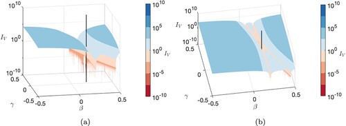
For each Taylor state belonging to this 2-parameter family, we calculate its rate of change assuming the alpha-effect of equation (4(4) $\alpha ={\alpha }_0\frac{729}{16}{r}^8(1-r^2{)}^2\cos \theta ,$(4) ) with ${\alpha }_0=18$. Figure 1 shows the surface of $I_V$ as a function of the two parameters, in the proximity of the known stable steady state demarcated by the vertical black line. We note how this point lies within an extended trough and hence that there are many Taylor states within this (restricted) parameter space for which $I_V$ is small enough to represent a rate of magnetic field change of $I_V<1$. This is a key and not a priori obvious result, that demonstrates the abundance of “quasi-steady” Taylor states: they are not only found at isolated locations in parameter space but exist continuously over significant ranges of parameters albeit in this example close to ${\mathit{B}}_d$.

Figure 1. Surface plot of the normalised instantaneous rate of change of magnetic field over the core volume, $I_V$, as a function of the l = 1, n = 1 and l = 1, n = 2 toroidal coefficients β and γ respectively. The vertical black line corresponds to the coefficient values of the known stable steady solution of Li et al. (2018). The α-effect form (4(4) $\alpha ={\alpha }_0\frac{729}{16}{r}^8(1-r^2{)}^2\cos \theta ,$(4) ) is used, with an above critical magnitude of ${\alpha }_0=18$. (a) and (b) show the same 3D plot viewed from a different angle (Colour online).

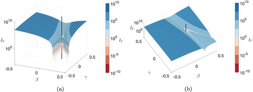
The bottom of the valley seen in figure 1 appears to have a “spiked” nature, with significant variation in some neighbouring values, despite the smooth broader trends. This is likely not to be of geophysical interest but rather merely an artefact of the uniform, finite-resolution grid that has been used. Despite the high-resolution grid used ($1000\times 1000$), the steepness of the valley edge and the lack of alignment between the trough and the grid cause relatively large fluctuations.

4. In search of stable steady Taylor states

Here we run dynamical simulations of the magnetostrophic equations to evolve Taylor-state magnetic fields with time, to numerically assess stability. All of these simulations use the code of Li et al. (2018) and are conducted at the sufficiently high resolution of maximum spherical-harmonic degree L = 50 and radial basis truncation N = 25. For the majority of the calculations in this section (all those reported in sections 4.1–4.4), the α-effect form (4(4) $\alpha ={\alpha }_0\frac{729}{16}{r}^8(1-r^2{)}^2\cos \theta ,$(4) ) is used, with an above critical magnitude of ${\alpha }_0=18$. The sensitivity of our results to this choice is then considered in section 4.5. There are several strands to our approach here. Firstly, we begin with simple initial conditions, purely within either the dipole or quadrupole symmetry. We analyse the evolution of these Taylor states observing whether the solution converges to a stable state, anticipating that at least some of our models will converge to the steady states ${\mathit{B}}_d$ and ${\mathit{B}}_q$, already reported by Wu and Roberts (2015) and Li et al. (2018). Secondly, we generalise this approach to mixed symmetry and evolve a large number of more complex initial conditions. Our aim here is to find a mixed-symmetry steady state. Thirdly, we adopt as an initial condition some of the many “quasi-steady” Taylor states we found in section 3, and so numerically assess their stability. Finally, we assess whether the known steady, stable states ${\mathit{B}}_d$ and ${\mathit{B}}_q$ of Wu and Roberts (2015) and Li et al. (2018) restricted to dipole or quadrapole symmetry are also stable in a mixed symmetry.

4.1. Searching within symmetry classes: single-mode initial conditions

We begin by using a very simple but unsteady initial Taylor state, that of a l = n = 1 purely poloidal mode, whose evolution is mapped out in terms of $I_V$ in figure 2.

Figure 2. The magnetostrophic trajectory of $I_V$ as a function of toroidal and poloidal energy (defined as half the squared integral over the unit sphere of the respective components). The initial condition is a single poloidal l = n = 1 mode, which is a simple but unsteady Taylor state. The solution evolves from the magenta data point toward a stable steady state with $I_V\ll 1$ and tending to zero. Two magnetic diffusion times of duration are plotted, with circular data points plotted at intervals of 0.001 and blue points denoting when $I_V>1$ and red points when $I_V<1$ (Colour online).

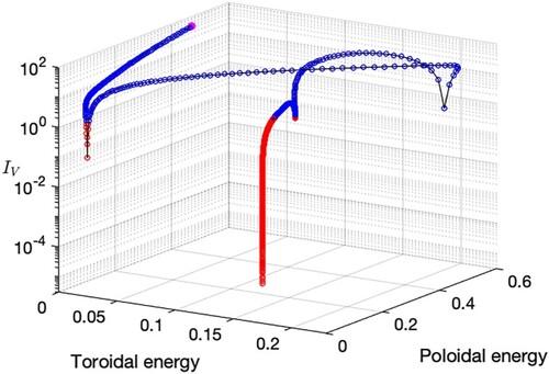
Initially, the rate at which the field changes is fast, with large changes in the poloidal and toroidal energies between each one-hundredth of a magnetic diffusion time, indicated by the red data points plotted. The field progresses from this initial state towards a stable steady Taylor state with a vanishingly small value of $I_V$. The evolution is not associated with purely monotonically decreasing $I_V$ but rather the trajectory enters and escapes several local minima, with $I_V\lesssim 1$ (thus indicating that quasi-steady states are not always stable or attracting) before approaching the vicinity of a stable point by t = 1 where $I_V=2\times {10}^{-1}$. For times t>1, we tracked the solution which continues to converge with $I_V<{10}^{-6}$.

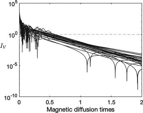
We now repeat the above procedure but for a suite of single poloidal mode initial conditions, for the complete set of different combinations of $(l,n)$ (within the triangular truncation with $L_{max}=50$ and $N_{max}=25$) this is a total of 650 simulations. For visual clarity, only 50 of these simulations are shown in figure 3. Single spherical-harmonic modes are used here as they allow us to explore a range of initial fields with different spatial scales that are always strictly in either dipole or quadrupole symmetry while being guaranteed to be an exact Taylor state (Livermore 2009). Each calculation is performed in either dipole (red lines) or quadrupole symmetry (black lines), as determined by the initial condition.

Figure 3. Graphs showing the evolution of (a) $I_V$ and (b) deviation in magnetic energy from the stable state within each symmetry ($\pm {\mathit{B}}_d$ or $\pm {\mathit{B}}_q$ respectively), for the suite of single poloidal mode initial conditions, which fall into either the dipole or quadrupole symmetry class.

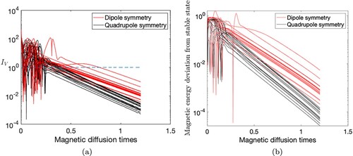
Within two magnetic diffusion times, all trajectories are convergent to attracting steady states and have an exponentially decreasing $I_V$. Because $\mathit{B}$ and $-\mathit{B}$ evolve identically, on ignoring the sign of the magnetic field all calculations converge to a single stable steady state within each symmetry class, those found by Wu and Roberts (2015), Li et al. (2018) and denoted as ${\mathit{B}}_d$ and ${\mathit{B}}_q$ here. Beyond the initial transient phase, whose duration varies with initial conditions, within each symmetry class all solutions converge at the same rate to the fixed point solution as shown by the same linear gradient on the plot for each colour.

The apparent convergence to only the two known steady stable states (or four steady states $\pm {\mathit{B}}_d$, $\pm {\mathit{B}}_q$ if the sign is included), suggests one of several explanations: that stable steady Taylor states are rare, that imposing purely dipolar or quadrupolar symmetry is too restrictive, or that the solutions we find are overwhelmingly attracting; each of these possibilities is explored in the following sections 4.2–4.4. The small number of two stable states that we found stands in stark contrast to the apparent ubiquity of quasi-steady Taylor states found in section 3.

4.2. Searching within symmetry classes: the evolution from quasi-steady Taylor states

We now address the issue of whether the rarity of stable states that we were able to find in the previous section was due to the simplistic nature of the single-mode initial conditions, which perhaps were too far from any stable state. We now describe a strategy for finding a suite of “quasi-steady” Taylor states using an optimisation method, which then are time-evolved to assess their stability.

The calculations of $I_V$ shown in figure 1 reveal many locations in the two-parameter subspace we explored where the fields are “quasi-steady”. We now generalise the approach to an m-dimensional subspace of Taylor states. As before, the poloidal field remains fixed to the poloidal component of the stable dipole-symmetry solution, ${\mathcal{S}}_0$. However, now the toroidal component of the field that we consider is much more general. The toroidal field is constructed by the choice of the coefficients of the m largest scale modes, $a_1,a_2,\dots a_m$, from within the domain $[-1,1]$ (which spans the poloidal coefficients values), and the rest of the toroidal field is determined through solving the linear system of Taylor's constraints, (13) $\begin{array}{rl}\mathit{B}& ={\mathcal{S}}_0+a_1{\mathcal{T}}_1+a_2{\mathcal{T}}_2+\cdots +a_m{\mathcal{T}}_m+a_{m+1}(a_1,a_2,\dots ,a_m,{\mathcal{S}}_0){\mathcal{T}}_{m+1}+\dots \\ & +a_n(a_1,a_2,\dots ,a_m,{\mathcal{S}}_0){\mathcal{T}}_n.\end{array}$(13) Here, ${\mathcal{T}}_i$ denotes a toroidal mode (within the chosen symmetry class), ordered from large-scale (low spherical-harmonic degree l, $l=1,n=1\dots N_{max}$) mode $i=1\dots m$, whose coefficients are varied throughout our search; to the remaining higher l toroidal modes (up to $l=L_{max},n=1\dots N_{max}$) denoted by subscripts $i+1,\dots ,n$ whose coefficients are determined through solving Taylor's constraints. This principle is akin to implementing a boundary condition using a spectral method by solving for the smallest scale modes (Boyd 2001).

The specific example reported here has a resolution of L = 10, N = 5; imposing Taylor's constraint requires 18 conditions to be satisfied. Here there are 50 toroidal coefficients, so we define a subspace using the remaining m = 32 parameters. We now search over the 32-dimensional subspace of Taylor states for those which have a small $I_V$. A direct grid-search method would be too time consuming, so here we use the neighbourhood algorithm optimisation (Sambridge 1999) to more efficiently locate the regions of small $I_V$. To initialise the algorithm, we choose p random models, for each we evaluate $I_V$. The domain is then divided up into p neighbourhoods (“Voronoi” cells in spectral space) surrounding each point and the q regions centred on the smallest values of $I_V$ retained to be explored further by repeating the process x times. At each stage, within each neighbourhood we explore p new models obtained by a uniform random walk within each of the Voronoi cells. The parameters p, q and x are input parameters suitably chosen to balance computational time and the amount of exploration. The algorithm results in a set of models which are clustered around local minima in $I_V$. Here, we explored the 32-dimensional space using p = 20, q = 10, x = 5. Of the resulting models, we choose the 68 magnetic fields with a value of $I_V$ below a threshold of 1 to be used as initial conditions. These quasi-steady Taylor states exhibit a range of poloidal and toroidal energies, spread throughout the ranges [0.01, 0.47] and [0.01, 0.43] respectively.

Figure 4(a) shows the evolution of two of these quasi-steady Taylor state magnetic fields within dipole symmetry, neither of which is close to ${\mathit{B}}_d$. Despite a low value of $I_V$, the magnetic fields diverge from the initial state before eventually converging to ${\mathit{B}}_d$. A similar behaviour is found within quadrupole symmetry (figure 4(b)).

Figure 4. The paths taken from two initial quasi-steady Taylor-state magnetic fields, within (a) dipole symmetry and (b) quadrupole symmetry using the α-effect form (4(4) $\alpha ={\alpha }_0\frac{729}{16}{r}^8(1-r^2{)}^2\cos \theta ,$(4) ) with ${\alpha }_0=18$. The fields diverge from the initial states (magenta points) before finally converging to ${\mathit{B}}_d$ and ${\mathit{B}}_q$ respectively. Blue points denote when $I_V>1$ and red points when $I_V<1$. In (b), the trajectory passes through multiple models which are quasi-steady but unstable. In both cases, convergence to the stable model is denoted by the continuous red line (Colour online).

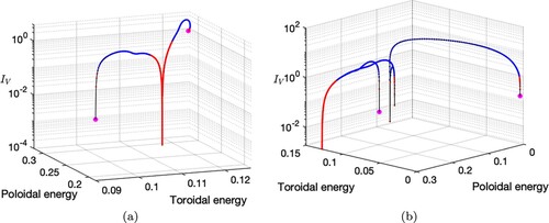
This instability of quasi-steady initial states is mirrored by all 68 models we found in our 32-dimensional subspace, strengthening the evidence that all (at least, all those we have explored) quasi-steady states are unstable, aside from ${\mathit{B}}_d$.

The same procedure is also carried out within the quadrupole symmetry, with similar results obtained. The many quasi-steady Taylor states are all unstable and ultimately converge to ${\mathit{B}}_q$ as shown in figure 4(b).

4.3. Mixed symmetry: stability of solutions

We now assess whether the restriction to a specific symmetry class influences the dynamics we have found. Of course, even by considering a general axisymmetric representation, should an initial field be purely dipole or quadrupole, then the solution will remain so indefinitely. However, if the initial field is of mixed symmetry (containing both dipolar and quadrupolar components) then these components interact and its evolution cannot be partitioned into that of its two symmetric components. We broaden our search for stable steady Taylor states without restriction to equatorial symmetry. To do so, we now use a much more general form of initial conditions and construct random Taylor states that have mixed symmetry and a combination of toroidal and poloidal modes.

We adopt an initial condition of a large-scale axisymmetric Taylor-state magnetic field of maximum degree L = 4, N = 2, which has 16 degrees of freedom; Taylor's condition requires 6 constraints that need to be satisfied. We assign the coefficients of the 10 largest scale modes to be randomly chosen from within the range $[-1,1]$ and solve the linear system of constraints for the remaining 6 coefficients. The magnetic field in this example has the following components (14) $\begin{array}{rl}\mathit{B}& =+a_{1,1}{\mathcal{S}}_{1,1}+a_{1,2}{\mathcal{S}}_{1,2}+a_{2,1}{\mathcal{S}}_{2,1}+a_{2,2}{\mathcal{S}}_{2,2}\\ & +a_{3,1}{\mathcal{S}}_{3,1}+a_{3,2}{\mathcal{S}}_{3,2}+a_{4,1}{\mathcal{S}}_{4,1}+a_{4,2}{\mathcal{S}}_{4,2}\\ & +b_{1,1}{\mathcal{T}}_{1,1}+b_{1,2}{\mathcal{T}}_{1,2}+b_{2,1}{\mathcal{T}}_{2,1}+b_{2,2}{\mathcal{T}}_{2,2}\\ & +b_{3,1}{\mathcal{T}}_{3,1}+b_{3,2}{\mathcal{T}}_{3,2}+b_{4,1}{\mathcal{T}}_{4,1}+b_{4,2}{\mathcal{T}}_{4,2},\end{array}$(14) where $a_{1,1},a_{1,2},a_{2,1},a_{2,2},a_{3,1},b_{1,1},b_{1,2},b_{2,1},b_{2,2},b_{3,1}$ are the coefficients that are assigned values and the coefficients of the higher degree modes $a_{3,2},a_{4,1},a_{4,2},b_{3,2},b_{4,1},b_{4,2}$ are calculated through solving Taylor's constraints.

We form a set of 1000 randomised Taylor states, which comprise the initial conditions for an ensemble of calculations. Each initial magnetic field will evolve along a different path and in doing so we will search through a much broader region of state space than we have done so far for attracting solutions.

The evolution of four initial conditions (which illustrate the typical behaviour of the ensemble) is plotted in figure 5. All solutions shown remain time-dependent and quasi-periodic. Importantly, none of the solutions from our large suite of calculations converge to a stable Taylor state, reinforcing the evidence that these states are very rare. In the mixed-symmetry case considered in this section, we fail to find any stable Taylor states, including those strongly attracting in the purely dipole or purely quadrupolar symmetry classes. This is important as it is undoubtedly the situation of greatest geophysical interest, as the Earth's magnetic field is complex and of mixed symmetry.

Figure 5. The evolution of four different initial conditions with mixed symmetry (black, blue, red, green) shown by (a) Magnetic energy and (b) $I_V$. The α-effect form (4(4) $\alpha ={\alpha }_0\frac{729}{16}{r}^8(1-r^2{)}^2\cos \theta ,$(4) ) was used with ${\alpha }_0=18$ (Colour online).

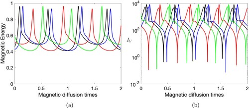
Another notable feature from these results is the plethora of troughs in the rate of change of magnetic field as the field evolves. The solution passes through fields which are “quasi-steady” as $I_V$ becomes smaller than 1. This confirms the results of previous sections, where we observed many different magnetic fields that were “quasi-steady”, but what we show here is that these states are in general not stable and given time will diverge.

Figure 5 also shows that although the trajectories are distinct (and are not simply offset in time), they show a remarkable degree of similarity. In particular, the peaks of magnetic energy (about one in our units) and of $I_V$ are approximately uniform over time, suggesting that the trajectories might all be close to a non-steady attractor.

4.4. The strength of the known symmetric solutions as attractors

The apparent lack of stable steady solutions in mixed symmetry suggests that the stable solutions of definite symmetry: ${\mathit{B}}_d$ and ${\mathit{B}}_q$ lose some of their attractive properties when embedded in the broader non-equatorially symmetric solution class.

Here, we investigate this by perturbing ${\mathit{B}}_d$ by a small quadrupolar component, breaking the purely dipole symmetry. When this perturbation has zero size, then the trajectory will not deviate from ${\mathit{B}}_d$. It is likely that small perturbations (whose size is below a threshold) will converge to ${\mathit{B}}_d$, but larger perturbations may always diverge. The structure of the perturbations must ensure that the whole magnetic field remains a Taylor state. This is simple to achieve by considering a purely toroidal, quadrupolar perturbation (Livermore et al. 2009), which for simplicity we define by taking all the non-zero (toroidal, odd-l) coefficients to be the same value. Working within the truncation L = 50, N = 25, and recalling the normalisation of our modes, this means that the perturbation has an energy of ${625}^2{q}^2/2$, compared with the unperturbed field with energy 0.368 (Li et al. 2018). We then define the perturbation magnitude by δ, as the ratio of the energy of the imposed quadrupolar field to the original dipolar field.

We find that there is a threshold of $\delta \approx {10}^{-2}$ below which an initial state will converge to ${\mathit{B}}_d$. For initial conditions with δ exceeding about ${10}^{-2}$ then the field fails to converge, as was seen in section 4.1. This same procedure is carried out for the allied case of dipolar perturbations to the quadrupolar field ${\mathit{B}}_q$, also resulting in a similar perturbation threshold.

Although a very special class of perturbation, this corroborates our finding that the steady states ${\mathit{B}}_d$ and ${\mathit{B}}_q$, stable and strongly attractive in their restricted symmetry classes, are only weakly attractive when embedded in a broader solution space. Therefore, this suggests that magnetostrophic models (at least with our choice of α) would not be expected to converge to any stable Taylor state when considering mixed symmetry.

4.5. The dependence on the choice of α-effect

Our analysis so far has been based on an α-effect, which is a valuable approach when studying axisymmetric dynamos. However, because the choice of α is arbitrary and to investigate whether our results have broader applicability, it is useful to explore varying both the magnitude and the spatial structure of the α-effect.

4.5.1. Magnitude of ${\alpha }_0$

The α-effect adopted in section 3 has a critical value of ${\alpha }_0=13.1$ (above which a generalised magnetic perturbation will grow); and a Taylorised critical value of ${\alpha }_T=13.8$ above which a Taylor-state perturbation will grow. We now reduce the strength of the α-effect from ${\alpha }_0=18$, to ${\alpha }_0=16$ (which remains above the critical value), to investigate the dynamics when the system is more weakly driven. The equivalent plot as figure 1 is shown in figure 6, with the stable solution of Li et al. (2018) at ${\alpha }_0=16$ indicated by the black line.

Figure 6. Surface plot of $I_V$ as a function of the l = 1, n = 1 and l = 1, n = 2 toroidal coefficients β and γ respectively. The vertical black line corresponds to the coefficient values of the known stable steady solution of Li et al. (2018). The α-effect form (4(4) $\alpha ={\alpha }_0\frac{729}{16}{r}^8(1-r^2{)}^2\cos \theta ,$(4) ) is used, with an above critical magnitude of ${\alpha }_0=16$. (a) and (b) show the same 3D plot viewed from a different angle.

Similarly, we repeat the dynamical simulations of section 4.3, now with ${\alpha }_0=16$ using the same 1000 random mixed-symmetry initial conditions (figure 7). This time we find that instead of failing to converge at all, the models all converge to the steady states ${\mathit{B}}_d$ and ${\mathit{B}}_q$ (Li et al. 2018). Therefore we have still failed to find any stable steady Taylor state that has the complexity of a mixed dipole and quadrupole symmetry. The difference in the case of ${\alpha }_0=16$ is merely the strength of attraction of these stable points appears stronger and therefore enables convergence from arbitrary initial conditions, unlike for ${\alpha }_0=18$, where we found that in order for the system to collapse to a symmetry class and hence find the stable point, the initial condition was required to be sufficiently close.

Figure 7. Normalised instantaneous rate of change of magnetic field within the core, $I_V$, with ${\alpha }_0=16$, for 60 different random initial conditions of mixed symmetry.

As ${\alpha }_0$ is increased further above critical (e.g. ${\alpha }_0=25$), the stronger forcing results in a large and rapidly growing magnetic field and ultimately in numerical instability. Although we have not investigated the source of the instability in detail, the issue may be specific to the axisymmetric problem we are studying, as in fully 3D models more powerful equilibration limits the magnetic field strength (Fearn and Rahman 2004b).

In summary, what we observe is no fundamental change in the conclusions of abundance of “quasi-steady” Taylor states, but a scarcity of stable steady Taylor states (and a complete absence in mixed symmetry). The difference discerned is merely that less strongly driven models allow magnetic fields to converge to stable steady states more easily, from a wider range of initial conditions.

4.5.2. Structure of the α-effect

We now investigate the effect of adopting an alternative structure for the α-effect using a similar suite of 1000 mixed-symmetry initial conditions. We use a more complex form (see Li et al. 2018) and a very simple structure $\alpha ={\alpha }_0\sqrt{\frac{7}{3}}\frac{343}{48}{r}^3(1-r^2{)}^2\cos (3\theta ),$ and $\alpha ={\alpha }_0\cos (\theta ),$ which are normalised such that $\max |\alpha |={\alpha }_0$ (as was the α-affect defined in equation (4(4) $\alpha ={\alpha }_0\frac{729}{16}{r}^8(1-r^2{)}^2\cos \theta ,$(4) )). This helps to allow a fair comparison, although note the critical values of ${\alpha }_0$ are in general distinct. In terms of generalised (not restricted to Taylor states) kinematic dynamos, the critical value has a slightly smaller value of ${\alpha }_0=12.5$ (Li et al. 2018) for the former and ${\alpha }_0=13.1$ (Fearn and Rahman 2004a) for the latter (the same as for the form of equation (4(4) $\alpha ={\alpha }_0\frac{729}{16}{r}^8(1-r^2{)}^2\cos \theta ,$(4) )). Qualitatively similar results are observed for all α-effect structures, we observe four types of behaviour dependent on the magnitude of ${\alpha }_0$: at values of ${\alpha }_0$ below critical, dynamo action fails and the field decays via magnetic diffusion; slightly above critical our models converge toward one of two stable states, of either dipole or quadrupole symmetry; more strongly forced models have continually and rapidly varying rates of change and fail to converge to a stable state (as shown in figure 5); while significantly super-critical values of ${\alpha }_0$ lead to high magnetic field rates of change and very large magnetic field energies.

5. Discussion

5.1. Comparison with Earth

We have focussed in this paper on a set of magnetostrophic models, under a variety of approximations such as axisymmetry and α-effect driving. It is of significant interest to compare these to the Earth, to try to identify whether Earth might be in a “quasi-steady”, “stable”, or other, state. Because the evolution of the geomagnetic field occurs on a large range of timescales, and in particular contains dynamics excluded from the magnetostrophic approximation such as inertia-driven waves causing rapid oscillations, a direct comparison is not straightforward. Nevertheless, here we discuss a series of comparisons of timescale between our models and Earth.

A direct and very simple comparison can be conducted by calculating the surface normalised timescale, $I_S$, based on the CHAOS-6 model at epoch 2015, itself based on satellite and ground-based data (Finlay et al. 2016). We find a value of $I_S=6\times {10}^7$ or in dimensional units $2.4\times {10}^{-4}{\mathrm{yrs}}^{-2}$. This is much larger than the rates of change we observe in our magnetostrophic models, due to the dominating short timescale secular variation that is explicitly excluded from our magnetostrophic model.

A better comparison can be made using archaeomagnetic models, which describe the Earth's magnetic field over the long timescales necessary to be compatible with Taylor-state dynamics. Figure 8 shows both the surface magnetic energy and $I_S$ based on the GGF100k model (Panovska et al. 2018) over the past 100,000 years. Although GGF100k is smoothed due to data sparsity, the figure shows that it contains a range of timescales which are still slightly faster (higher $I_S$), than the range of timescales of the two magnetostrophic models presented. Interestingly, this demonstrates that the slowest dynamics captured in GGF100k could be magnetostrophic in origin, at least in terms of timescale.

Figure 8. Observational geomagnetic field data from GGF100k (Panovska et al. 2018) are compared to two illustrative models. (a) Total magnetic field core surface energy over the past 100 ka. (b) The instantaneous rate of change of magnetic field at Earth's surface $I_S$ (defined in equation 11(11) $I_V=\frac{\int {\dot{\mathit{B}}}^2\mathrm{d}V}{\int {\mathit{B}}^2\mathrm{d}V},\mathrm{and}{I}_S=\frac{\int {\dot{\mathit{B}}}^2\mathrm{d}S}{\int {\mathit{B}}^2\mathrm{d}S},$(11) ), the GGF100k model, and the resultant field dynamics after passing the data through a Butterworth filter with a 50,000 yr timescale cutoff (red), are compared to the results from the mixed-symmetry simulations of section 4.3 (blue and green). The offset time of GGF100k is arbitrarily chosen to be 0 (Colour online).

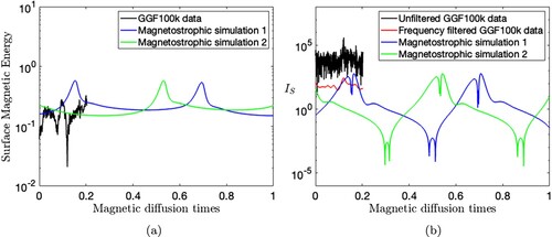
To make a still better comparison, we need to filter out the most rapid timescales (presumably caused by non-magnetostrophic dynamics) from the GGF100k model. To do this, we adopt a Butterworth filter with a 50,000 yr cutoff timescale, which retains only timescales at or above 50,000 yrs (see the red line in figure 8). This timescale, $\tau /{\pi }^2$, is the e-folding time of the slowest mode of Ohmic decay when considering the effects of the spherical geometry (Backus 1958) and so is a dynamically relevant threshold. The filtered GGF100k model is now consistent with the magnetostrophic models in terms of timescale, although it does not show the large fluctuations that we found in our numerical models.

What these comparisons highlight is the difficulty in extracting the magnetostrophic component of Earth's magnetic field from observational models. Part of the difficulty is the broad range of timescales that the magnetostrophic system requires, and so a low-pass filter at any given frequency will likely not succeed. The magnetostrophic system includes slow dynamics such as diffusion (with timescales of c.a. 50 ka), but also possibly much more rapid features like MC waves with timescales 100–10,000 yr depending on the complexity of the magnetic field (Finlay et al. 2010). At the very rapid end of the spectrum, decadal timescales may even overlap with those of non-magnetostrophic dynamics such as the torsional waves, making separation based purely on timescales very challenging indeed. Without a clear way to separate the magnetostrophic signal, it is not possible to quantify a value of $I_S$ for the magnetostrophic component of the geodynamo, and therefore to assess how it compares with the models that we have described in this paper.

It is interesting to consider how magnetostrophic dynamics may differ from those in the geodynamo, where inertia and viscosity play a role. Inertia often acts as a restoring force, acting on short timescales and causing a rapid response to perturbations in the system. For example, it permits torsional waves, which act to re-establish the unperturbed state (Jault and Finlay 2015). In the absence of this correction mechanism, deviations from the long-term equilibrium state may be expected to persist, perhaps through the slow build-up of an unfavourable state followed by a rapid re-equilibration. Such rapid changes are exacerbated by the lack of viscosity which ordinarily would promote the diffusion of small-scale features in the fluid and smooth out temporal dynamics. Inviscid models such as ours might therefore be expected to contain more extreme variations than weakly viscous counterparts. It is therefore quite possible that the periods of slow change that our models predict disappear on reinstating weak inertia and viscosity.

6. Concluding remarks

It has been previously shown that there is a large space of magnetic fields that exactly satisfy Taylor's constraint instantaneously (Livermore et al. 2009, Hardy et al. 2020). In this study, we have addressed the question of which of these are steady and stable, from a variety of standpoints.

Firstly, we have shown that there exists a large space of Taylor states which are quasi-steady, with a rate of change of the core surface field $I_S$ of 1 or below. Secondly, we find that stable steady Taylor states are very rare. Within specific imposed symmetries of either dipole or quadrupole, only a single stable state is found. Crucially, in the more general and physically relevant situation: without any symmetrical restrictions, then our extensive search for any stable states is fruitless. This suggests that it may be the case that no stable steady Taylor states with a mixed symmetry exist except for very weak forcing.

Of course, despite using a wide range of initial conditions, across a range of spatial scales, we can not rule out the possibility that some stable Taylor states do exist, but that they are merely not sufficiently strong attractors for us to find. Also, we emphasise that all our calculations are restricted to axisymmetry, and the full three-dimensional setting might yield different results.

The mean field α-effect used to provide the driving force for our axisymmetric dynamos acts as a non-ideal proxy for buoyancy. Coupling the Navier–Stokes equation with the full temperature equation would drive more complex non-linear interactions with perhaps more feedback and stronger equilibration. Alternatively, as a more direct and simple extension to our model, buoyancy non-linearities can also be introduced through α-quenching. In this setting, the value of α is no longer fixed but allowed to evolve subject to the magnetic feedback leading to deformation of the turbulence (Rüdiger and Kichatinov 1993). The addition of a quenching of the α-effect is of course an approximation. However, the inclusion of a simple algebraic form, such as $\alpha =\frac{{\alpha }_0}{1+B^2/B_0^2}$ of Kleeorin et al. (2000), where $B_0$ is the equipartition field strength, would allow an initial study into any stabilising effect.

The stability of mean field dynamos has been previously examined within finite viscosity models. Fearn and Rahman (2004a) studied the ${\alpha }^2$-dynamo model at (relatively large) finite Ekman numbers of about $4\times {10}^{-4}$ and compared the behaviour within a three-dimensional non-axisymmetric non-linear system and the two-dimensional axisymmetric case. They reported very different behaviour in these two situations: in the axisymmetric case the magnetic energy grows quickly as the forcing ${\alpha }_0$ is increased (for values above critical), whereas in the 3D case the field is more rapidly equilibrated by the fully 3D treatment of the non-linear interaction between the field and the flow. This agrees with our findings in section 4.5 that axisymmetric and strongly forced models result in very strong magnetic fields that become increasingly computationally expensive and prone to instability. Therefore caution is required when interpreting axisymmetric studies such as ours in the context of the three-dimensional geomagnetic field. The variability of stability as a function of Ekman number has been studied by Hollerbach and Ierley (1991), who investigated the asymptotically small limit of viscosity in an ${\alpha }^2$-dynamo model. For all α-effects considered their solutions do approach a Taylor state in this limit. However, the manner of the transition from the viscous to inviscid regime varies. The formal limit $E\to 0$ is seen to not always be well-behaved, sometimes requiring a discontinuous jump.

Finally, there have been many suggestions of a marked difference in the fluid behaviour in magnetostrophic and finitely viscous models (McLean et al. 1999). While not definitively proven, the plausible intuition remains that the dynamo is particularly unstable as $E\to 0$ (Zhang and Gubbins 2000), as in the absence of viscous damping to suppress perturbations, stable states are less likely to be sustained. Instability can arise due to dynamo action being extremely sensitive to the vigour of convection by which it is driven (the difference between the Rayleigh number and its critical value). Zhang and Gubbins (2000) showed that at small Ekman numbers the critical Rayleigh number is increasingly sensitive to the poloidal magnetic field. Therefore small fluctuations in the magnetic field will directly lead to rapid variations in the strength of convection and significantly alter the state of the dynamo. The nature of the Earth's core being at parameter values unattainable in viscous numerical simulations ($E={10}^{-15}$) makes it very challenging to accurately model the stability of the geodynamo. While magnetostrophic models (at E = 0) may be over-sensitive to instabilities, all present finite viscosity ($E>{10}^{-9}$) models have the opposing problem of inherently being more stable than the geodynamo itself, as the inflated significance of viscosity is expected to provide an artificial stabilising effect. Therefore the question of the stability of a realistic model of the Earth's magnetic field, still computationally out of reach, remains open. The construction of a fully three-dimensional Taylor-state dynamo model driven by thermal convection is an obvious but significant future objective. This would be a profound step forward, facilitating direct comparisons between viscous and inviscid dynamos as we attempt to constrain the behaviour in Earth's core.

Disclosure statement

No potential conflict of interest was reported by the author(s).

Additional information

Funding

This work was supported by the Engineering and Physical Sciences Research Council (EPSRC) Centre for Doctoral Training in Fluid Dynamics at the University of Leeds under Grant No. EP/L01615X/1. C.M.H. acknowledges funding from the European Research Council (agreement 833848-UEMHP) under the Horizon 2020 programme. P.W.L. acknowledges partial support from Natural Environment Research Council (NERC) grant NE/G014043/1.

References

- Abdel-Aziz, M. and Jones, C., αω-dynamos and Taylor's constraint. Geophys. Astrophys. Fluid Dyn. 1988, 44, 117–139.
- Amit, H., Leonhardt, R. and Wicht, J., Polarity reversals from paleomagnetic observations and numerical dynamo simulations. Space Sci. Rev. 2010, 155, 293–335.
- Aubert, J., Recent geomagnetic variations and the force balance in Earth's core. Geophys. J. Int. 2020, 221, 378–393.
- Aubert, J. and Gillet, N., The interplay of fast waves and slow convection in geodynamo simulations nearing Earth's core conditions. Geophys. J. Int. 2021, 225, 1854–1873.
- Aurnou, J. and King, E., The cross-over to magnetostrophic convection in planetary dynamo systems. Proc. R. Soc. A: Math. Phys. Eng. Sci. 2017, 473, 20160731.
- Backus, G., A class of self-sustaining dissipative spherical dynamos. Ann. Phys. 1958, 4, 372–447.
- Boyd, J., Chebyshev and Fourier Spectral Methods, 2001 (New York: Dover).
- Cowling, T., The magnetic field of sunspots. Mon. Not. R. Astr. Soc. 1933, 94, 39–48.
- Davies, C. and Constable, C., Rapid geomagnetic changes inferred from Earth observations and numerical simulations. Nat. Commun. 2020, 11, 1–10.
- Davies, C., Pozzo, M., Gubbins, D. and Alfè, D., Constraints from material properties on the dynamics and evolution of Earth's core. Nat. Geosci. 2015, 8, 678–685.
- Driscoll, P. and Olson, P., Polarity reversals in geodynamo models with core evolution. Earth Planet. Sci. Lett. 2009, 282, 24–33.
- Fearn, D., Hydromagnetic flow in planetary cores. Rep. Prog. Phys. 1998, 61, 175–235.
- Fearn, D. and Proctor, M., Dynamically consistent magnetic fields produced by differential rotation. J. Fluid Mech. 1987, 178, 521–534.
- Fearn, D. and Rahman, M., Evolution of non-linear α2-dynamos and Taylor's constraint. Geophys. Astrophys. Fluid Dyn. 2004a, 98, 385–406.
- Fearn, D. and Rahman, M., Instability of non-linear α2-dynamos. Phys. Earth Planet. Inter. 2004b, 142, 101–112.
- Finlay, C., Dumberry, M., Chulliat, A. and Pais, M.A., Short timescale core dynamics: theory and observations. Space Sci. Rev. 2010, 155, 177–218.
- Finlay, C., Olsen, N., Kotsiaros, S., Gillet, N. and Toeffner-Clausen, L., Recent geomagnetic secular variation from Swarm and ground observatories as estimated in the CHAOS-6 geomagnetic field model. Earth Planets Space 2016, 68, 1–18.
- Gillet, N., Jault, D., Canet, E. and Fournier, A., Fast torsional waves and strong magnetic field within the Earth's core. Nature 2010, 465, 74–77.
- Hardy, C., Livermore, P., Niesen, J., Luo, J. and Li, K., Determination of the instantaneous geostrophic flow within the three-dimensional magnetostrophic regime. Proc. R. Soc. A: Math. Phys. Eng. Sci. 2018, 474, 20180412.
- Hardy, C., Livermore, P. and Niesen, J., Enhanced magnetic fields within a stratified layer. Geophys. J. Int. 2020, 222, 1686–1703.
- Hollerbach, R., On the theory of the geodynamo. Phys. Earth Planet. Inter. 1996, 98, 163–185.
- Hollerbach, R. and Ierley, G., A modal α2-dynamo in the limit of asymptotically small viscosity. Geophys. Astrophys. Fluid Dyn. 1991, 56, 133–158.
- Hollerbach, R., Barenghi, C.F. and Jones, C.A., Taylor's constraint in a spherical αω-dynamo. Geophys. Astrophys. Fluid Dyn. 1992, 67, 3–25.
- Jault, D. and Finlay, C., Waves in the core and mechanical core-mantle interactions. In Treatise on Geophysics: Core Dynamics, edited by G. Schubert, pp. 225–245, 2015 (Elsevier: Amsterdam).
- Kleeorin, N., Moss, D., Rogachevskii, I. and Sokoloff, D., Helicity balance and steady-state strength of the dynamo generated galactic magnetic field. Astron. Astrophys. 2000, 361, L5–L8.
- Li, K., Jackson, A. and Livermore, P., Taylor state dynamos found by optimal control: axisymmetric examples. J. Fluid Mech. 2018, 853, 647–697.
- Livermore, P., A compendium of galerkin orthogonal polynomials. 2009, Technical report, Scripps Institute of Oceanography. Available online at: http://escholarship.org/uc/item/9vk1c6cm.
- Livermore, P. and Hollerbach, R., Successive elimination of shear layers by a hierarchy of constraints in inviscid spherical-shell flows. J. Math. Phys. 2012, 53, 073104.
- Livermore, P., Jones, C.A. and Worland, S., Spectral radial basis functions for full sphere computations. J. Comput. Phys. 2007, 227, 1209–1224.
- Livermore, P., Ierley, G. and Jackson, A., The structure of Taylor's constraint in three dimensions. Proc. R. Soc. A: Math. Phys. Eng. Sci. 2008, 464, 3149–3174.
- Livermore, P., Ierley, G. and Jackson, A., The construction of exact Taylor states. I: the full sphere. Geophys. J. Int. 2009, 179, 923–928.
- Livermore, P., Ierley, G. and Jackson, A., The construction of exact Taylor states II: the influence of an inner core.. Phys. Earth Planet. Inter. 2010, 178, 16–26.
- Livermore, P., Ierley, G. and Jackson, A., The evolution of a magnetic field subject to Taylor's constraint: a projection operator applied to free decay. Geophys. J. Int. 2011, 187, 690–704.
- Malkus, W. and Proctor, M., The macrodynamics of α-effect dynamos in rotating fluids. J. Fluid Mech. 1975, 67, 417–443.
- McLean, D., Fearn, D. and Hollerbach, R., Magnetic stability under the magnetostrophic approximation. Phys. Earth Planet. Inter. 1999, 111, 123–139.
- Meduri, D.G., Biggin, A.J., Davies, C.J., Bono, R.K., Sprain, C.J. and Wicht, J., Numerical dynamo simulations reproduce paleomagnetic field behavior. Geophys. Res. Lett. 2021, 48, e2020GL090544.
- Olson, P., Coe, R., Driscoll, P., Glatzmaier, G. and Roberts, P., Geodynamo reversal frequency and heterogeneous core–mantle boundary heat flow. Phys. Earth Planet. Inter. 2010, 180, 66–79.
- Panovska, S., Constable, C. and Korte, M., Extending global continuous geomagnetic field reconstructions on timescales beyond human civilization. Geochem. Geophys. Geosyst. 2018, 19, 4757–4772.
- Parker, E., Hydromagnetic dynamo models. Astrophys. J. 1955, 122, 293–314.
- Proctor, M., On the eigenvalues of kinematic alpha-effect dynamos. Astron. Nachr. 1977, 298, 19–25.
- Roberts, P., Kinematic dynamo models. Philos. Trans. R. Soc. A 1972, 272, 663–698.
- Roberts, P. and Wu, C., On the modified Taylor constraint. Geophys. Astrophys. Fluid Dyn. 2014, 108, 696–715.
- Roberts, P. and Wu, C., On magnetostrophic mean-field solutions of the geodynamo equations. Part 2. J. Plasma Phys. 2018, 84, 735840402, 1–25.
- Roberts, P. and Wu, C., On magnetostrophic dynamos in annular cores. Geophys. Astrophys. Fluid Dyn. 2020, 114(3), 356–408.
- Rüdiger, G. and Kichatinov, L., Alpha-effect and alpha-quenching. Astron. Astrophys. 1993, 269, 581–588.
- Sambridge, M., Geophysical inversion with a neighbourhood algorithm – I. Searching a parameter space. Geophys. J. Int. 1999, 138, 479–494.
- Schaeffer, N., Jault, D., Nataf, H.C. and Fournier, A., Turbulent geodynamo simulations: a leap towards Earth's core. Geophys. J. Int. 2017, 211, 1–29.
- Schwaiger, T., Gastine, T. and Aubert, J., Relating force balances and flow length scales in geodynamo simulations. Geophys. J. Int. 2021, 224, 1890–1904.
- Soward, A. and Jones, C., α2-dynamos and Taylor's constraint. Geophys. Astrophys. Fluid Dyn. 1983, 27, 87–122.
- Tarduno, J., Cottrell, R., Davis, W., Nimmo, F. and Bono, R., A hadean to paleoarchean geodynamo recorded by single zircon crystals. Science 2015, 349, 521–524.
- Taylor, J., The magneto-hydrodynamics of a rotating fluid and the Earth's dynamo problem. Proc. R. Soc. A: Math. Phys. Eng. Sci. 1963, 9, 274–283.
- Wu, C. and Roberts, P., On magnetostrophic mean-field solutions of the geodynamo equations. Geophys. Astrophys. Fluid Dyn. 2015, 109, 84–110.
- Zhang, K. and Gubbins, D., Is the geodynamo process intrinsically unstable? Geophys. J. Int. 2000, 140, F1–F4.