On the mathematical theory of plumes

ABSTRACT

We reconsider the theory of turbulent plume formation provided by Schmidt (1941a,b) and its integral formulation, particularly that of Morton et al. (1956). A particular issue for the correct formulation of a mathematical theory is whether the plume is taken to have finite or infinite width, and whether the entrainment rate is prescribed or deduced. Fox (1970) showed that the entrainment rate for a plume can be deduced from the governing partial differential equations by the use of integral moment theory, providing one assumes expressions for the velocity and buoyancy profiles, but it is less clear if entrainment needs to be prescribed if the plume is taken to be of infinite width (as might be appropriate for a laminar plume). Here we choose an eddy viscosity model of a plume which differs from those previously used by allowing the eddy viscosity to vanish with the vertical velocity. We then show that for the ordinary differential equations describing the similarity solution for such a plume rising in an unstratified medium, their solution implies that the plume is finite, and that the entrainment rate at the plume edge is a consequence of the model formulation, and does not need to be hypothesised; and we also show that the entrainment coefficient which is thus determined is consistent with values obtained by experiment. We also show that the resulting velocity profiles differ from those found experimentally by their omission of the Gaussian tail, and we suggest that this discrepancy may be resolved in the model by the inclusion of the small molecular kinematic viscosity.

KEYWORDS:

• Plumes
• entrainment condition
• Schmidt theory
• eddy viscosity

1. Introduction

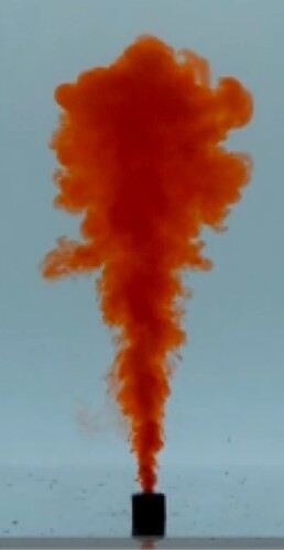
A plume is an isolated convective upwelling. Examples are the rise of smoke from an industrial chimney, the formation of cumulus clouds over oceans, ‘black smokers’ at mid-ocean rise vents, and explosive volcanic eruptions. In these examples, a source of buoyancy at (essentially) a point drives a convective flow in the fluid above. As suggested in figure 1, the plume forms a turbulent, approximately conical region, with a fairly sharp boundary. The turbulence causes rapid convective mixing, and allows us to conceptualise the plume as a relatively homogeneous cloud of density $\rho ={\rho }_0-\mathrm{\Delta }\rho$ rising through an ambient medium of density ${\rho }_0$. If ${\rho }_0$ depends on height z, then the medium is called a stratified medium, and it is stably stratified if ${\rho }_0^{\prime }\left(z\right)<0$.

Figure 1. A laboratory plume. Photograph courtesy Andy Woods.

1.1. Classical plume theory

The theory to describe the motion of a turbulent plume was apparently first properly formulated by Schmidt (1941a,b), and his model will be revisited below. The problem was evidently of then current interest, and there is an earlier paper by Zeldovich (1937) (see Zeldovich 1992), in which the important concepts of conserved integrals and self-similarity are introduced. Fox (1970) comments that the assumption of similarity was common to all plume theories then, based on experimental observation, although this is not theoretically consistent in a stratified medium. The first of Schmidt's two papers (but really one paper in two separated parts) considers the two-dimensional motion due to a line source, and the second considers the cylindrically symmetric plume emanating from a point source. Schmidt not only formulated the model, he solved it to the extent that he could, providing the appropriate similarity form of the equations and their solution in the form of power series, and additionally compared his results with experiments which he conducted himself.

Schmidt's theory used an eddy viscosity and thermal diffusivity based on Prandtl's mixing-length theory, and his choice of viscosity is discussed later. Schmidt was working at a Kaiser Wilhelm-Institut in Bochum during the second world war (after the war these became the Max Planck institutes), although there is no mention of military issues in his two papers. The papers came to the attention of G. I. Taylor, who studied them intently and used them as the inspiration for his report (Taylor 1945) for the U. S. Atomic Energy Commission, of which more below.

The study of cylindrical plumes formed the basis for C.-S. Yih's doctoral thesis, the main results of which are reported by Rouse et al. (1952). The authors essentially repeat Schmidt's work, apparently only discovering it when their paper was in the press. They provide the same model (but do not solve it), allowing the flow field to extend to infinity in the radial direction, and derive evolution equations for the momentum, buoyancy and kinetic energy fluxes, and display the self-similar form of the solutions. They also conduct experiments, and fit the buoyancy and upflow cross-sectional profiles with Gaussians.

There was a good deal of other interest in plumes at the time, much of it motivated by meteorological phenomena, for example Sutton (1948), Railston (1954) and Priestley and Ball (1955). This last paper followed the approach of Rouse et al. (1952), but considered also a stratified atmosphere, of obvious practical interest, but rendering the straightforward similarity approach untenable, since the scale height of the atmosphere provides a natural vertical length scale.

Batchelor (1954) provides a review of the subject (and many other subjects). His comment on Schmidt's work is somewhat caustic: he “gave an analysis of the mixing-length type, but I do not think such an analysis can be regarded as satisfactory at the present time”, although he does not elaborate. Batchelor's treatment of entrainment was presumably based on discussions with his mentor G. I. Taylor, whose 1945 report had explicitly introduced the concept. The matter came to a head when two of Batchelor's junior colleagues fused their work with Taylor's to produce what is undoubtedly the watershed paper in the subject, that of Morton et al. (1956). It is probably fair to say that many people would place this paper as the foundation of the modern theory of plume dynamics. It is discussed further below.

Schmidt's version of the model, as point forms of the equations, and including eddy viscous and diffusive terms, remains influential (e.g., Yih 1977), but its connection to the Morton–Taylor–Turner paper has become more opaque with time. Reviews of the subject do include discussion of this early material (e.g., Hunt and Van Den Bremer 2011, Farrugia and Micallef 2014), and the proper point forms of the equations remain of use, both in deriving suitable averaged equations (van Reeuwijk and Craske 2015, Woodhouse et al. 2016), or in direct numerical simulations (Marjanovic et al. 2017, 2019). On the other hand, for some this material has simply disappeared: for example, Rooney and Linden (1996) state that the “initial work on isolated sources of buoyancy was performed by Batchelor (1954), and Morton et al. (1956)”. A question we wish to address in this paper is: does this loss of connection matter?

1.2. Averaged plume theory

The Morton et al. (1956) paper was a landmark in the development of plume theory. Scase et al. (2006) comment that at that time it had been cited 639 times; in April 2021, that number had grown to something in excess of 1,600. It was firmly rooted in the literature of the time, introducing integral quantities, similarity, and Taylor's concept of entrainment. It differed from the Rouse et al. (1952) and Priestley and Ball (1955) papers by considering mass flux rather than energy flux; the merits of this choice were discussed by Morton (1971). Morton et al. (1956) were motivated (as was Taylor 1945) by the inapplicability of Schmidt's earlier similarity theory to stratified fluids (his 1945 work being precisely directed to the calculation of the rise height of an explosive fireball). But the paper also makes the comment, similar to that of Batchelor (1954) cited above, that “because of its dependence on mixture length theories and of the arbitrary assumptions that have to be made, the necessary labour would not be justified”. One senses an inherent distrust of the Prandtl theory of turbulence.

The idea of entrainment was abruptly suggested by Taylor (1945),¹ who was already aware of (and apparently motivated by) the work of Schmidt (1941a,b). In Morton et al.'s (1956) description, entrainment occurs at the finite plume radius, whereas the various kinds of diffusive model commonly describe the “plume” as formally extending to infinity (e.g., Vázquez et al. 1996), as seems appropriate if the effective viscosity (or Reynolds stress) does not vanish at the apparent edge. The basis for the entrainment assumption is that it agrees with experimental findings (e.g., Carazzo et al. 2006). Various authors have used a combination of experimental results and integral conservation laws to calculate values of the consequent entrainment coefficient (Fox 1970, Kaminski et al. 2005, van Reeuwijk and Craske 2015). We shall come back to this result below.

Much of the plume literature since 1956 has taken the Morton et al. (1956) paper as a starting point. Unsurprisingly, this is the case for the two junior authors (Morton 1959, Morton and Middleton 1973, Turner 1962, 1969, 1973, 1986). In his 1969 review, Turner cites Schmidt's papers, but follows Batchelor's (1954) earlier suggestion, that such calculations “entail some questionable assumptions about the turbulence distribution across the plume”. This view is repeated in his influential book (Turner 1973), where Rouse et al.'s (1952) paper is quoted, but not Schmidt's.

The natural result of this is that the subsequent literature has taken the Morton et al. (1956) paper as the starting point; this can be seen for example in the papers of Caulfield and Woods (1995), Hunt and Kaye (2001), Middleton (1975), Morton (1959), Morton and Middleton (1973), Turner (1962), Van den Bremer and Hunt (2010), and no doubt many others. The absence in these averaged models based on integral conservation laws of the eddy viscous terms can lead to illogicality, as for example in the exposition of Linden (2000), where the point forms of the governing equations are provided as for an inviscid fluid (presumably on the basis that the viscous terms are small), and the integral conservation laws are then discussed, based on these point forms. This is actually misleading, as the inviscid point forms can be solved, but the solutions are very un-plume-like.

Although it is never mentioned by Morton et al. (1956), the Morton–Taylor–Turner theory is of a type similar to other approximate methods to solve boundary layer flows, such as Pohlhausen's method for shear flows (Schlichting 1979). Given the absence of computing resources at the time, such methods were necessary, although now rarely used. A more up to date analogy is the use of cross-sectional averaging to describe two-phase pipe flows (e.g., Drew and Passman 1999), and indeed, such an averaging approach has been used in describing two-phase plumes (Tomàs et al. 2016). We will return to this analogy below.

There have been many developments of the Morton–Taylor–Turner theory, and one particular one of note is the extension to time-dependent plumes (Delichatsios 1979, Yu 1990, Scase et al. 2006). These models started with the point forms of the equations omitting Reynolds stress terms, and were later discovered to be ill-posed (Scase and Hewitt 2012). Interestingly, this last paper provided a resolution for the ill-posedness by introducing longitudinal dispersion due to eddy viscous effects. This is a rather contortionist exit, insofar as the dominant lateral stresses are ignored, but the small longitudinal ones are brought back. However, the correct resolution appears to be the omission of a suitable ‘profile coefficient’ to represent the cross-sectional velocity profile (Craske and Van Reeuwijk 2016, Woodhouse et al. 2016). Such profile coefficients are commonly used in two-phase flows to avoid ill-posedness, which arises for similar reasons (e.g., Fowler 1997).

Our purpose in this paper is to revisit the Schmidt theory, to examine it from a more mathematical viewpoint, and to ask whether it contains elements that can throw insight on to the theory of plumes. The traditional approach in plume theory is exemplified by Fox (1970). There are point forms of the equations, from which integration yields ordinary differential equations for mass flux, momentum flux and buoyancy flux. Taylor's hypothesis of entrainment is accepted, and values of the entrainment coefficient can be found by using a further integral constraint corresponding to conservation of kinetic energy. The subsequent effort becomes one of connecting experimental results to these derived integral constraints. It is our contention that this procedure glosses over the mathematical structure of the model, and so our focus is on this more fundamental aspect, rather than pursuing the goal of developing an improved model comparison with experiment; indeed it will become clear that our results fall short of a satisfactory comparison with experiment. In the following section we introduce what we call the viscous plume theory, explicitly including eddy-diffusive terms in the horizontal direction. We then work our way through its analysis from a modern perspective.

2. Viscous plume theory

The simplest mathematical model of a statistically steady turbulent plume is a cylindrically symmetric flow of radius $r=b\left(z\right)$, in which we use cylindrical coordinates $(r,z)$, with corresponding velocity components $(u,w)$ (thus the upwards fluid velocity is w). The plume rises through a medium of density ${\rho }_0\left(z\right)$. The basic Reynolds-averaged model is then given by (1a) $\begin{array}{rl}(ru{)}_r+r{w}_z& =0,\end{array}$(1a) (1b) $\begin{array}{rl}u{u}_r+w{u}_z& =-\frac{1}{{\rho }_0}{p}_r+\frac{1}{r}(r{\tau }_{\parallel }{)}_r,\end{array}$(1b) (1c) $\begin{array}{rl}u{w}_r+w{w}_z& =-\frac{1}{{\rho }_0}{p}_z-\frac{\rho }{{\rho }_0}g+\frac{1}{r}(r{\tau }_{\perp }{)}_r,\end{array}$(1c) (1d) $\begin{array}{rl}u{\rho }_r+w{\rho }_z& =\frac{1}{r}(rI{)}_r.\end{array}$(1d) These equations represent respectively conservation of mass, momentum (horizontal and vertical), and buoyancy; p is the pressure, ρ is the density, ${\rho }_0$ is the reference density of the surrounding ambient fluid, and g is the acceleration due to gravity. In writing (1(1a) $\begin{array}{rl}(ru{)}_r+r{w}_z& =0,\end{array}$(1a) ), we have made the Boussinesq approximation, which is based on the assumption that $\mathrm{\Delta }\rho$ is small, $\mathrm{\Delta }\rho \ll {\rho }_0$, where the density deficit $\mathrm{\Delta }\rho$ in the plume is defined as (2) $\mathrm{\Delta }\rho ={\rho }_0-\rho .$(2) We have included radial transport terms (but not the smaller longitudinal terms) which represent the effects of turbulent mixing: the stresses in (1(1a) $\begin{array}{rl}(ru{)}_r+r{w}_z& =0,\end{array}$(1a) ) are the Reynolds stresses (divided by density) (3) ${\tau }_{\parallel }=-\overline{u^{\prime }{}^2},{\tau }_{\perp }=-\overline{u^{\prime }{w}^{\prime }},$(3) and the equivalent buoyancy transport term (4) $I=-\overline{u^{\prime }{\rho }^{\prime }},$(4) where the primes denote turbulent fluctuations, and the overbars suitable averages (e.g., ensemble averages).

In order to form a closed mathematical theory, closure choices for these transport terms must be made. In due course we will choose the simplest such closures, in which a turbulent eddy diffusivity is introduced, so that (for a slender flow) (5) $-\overline{u^{\prime }{}^2}\approx {\nu }_T^{}\frac{\mathrm{\partial }u}{\mathrm{\partial }r},-\overline{u^{\prime }{w}^{\prime }}\approx {\nu }_T^{}\frac{\mathrm{\partial }w}{\mathrm{\partial }r},-\overline{u^{\prime }{\rho }^{\prime }}={\nu }_T^{}\frac{\mathrm{\partial }\rho }{\mathrm{\partial }r},$(5) and we will comment further on the choice of an eddy diffusivity below. Using the same coefficient ${\nu }_T^{}$ in the last term assumes a turbulent Prandtl or Schmidt number equal to one; this assumption is made for simplicity. The longitudinal mixing terms are neglected on the basis of our imminent assumption that the plume is thin; this assumption will be quantified below. Commonly, the model is written in the above form (with or without the eddy viscosity closure), with longitudinal gradients neglected (e.g., Fox 1970, Vázquez et al. 1996, Agrawal and Prasad 2003, Kaminski et al. 2005).

The buoyancy equation requires some comment. It caters for the fact that the density deficit in plumes may arise because of temperature, dissolved concentrations or particulate load, or a combination of these factors. But in all such cases, the turbulent conservation field for the relevant variable is simply based on advection and diffusion; for example we would have $T_t+\mathit{u}.\mathbf{\nabla }T=\mathbf{\nabla }.\left[{\nu }_T^{}\mathbf{\nabla }T\right]$ for temperature, and similarly for particulate or solute concentrations. Thus the buoyancy conservation equation simply represents this fact, together with the assumption that the density is an algebraic function of the conserved quantities. In certain circumstance, the veracity of this assumption may need to be examined further. For example, in a volcanic ash-laden plume, the eruption column has a density which is dependent on both temperature and ash concentration, and it rises through a surrounding stratified atmosphere whose stratification is itself determined by the relation of density to temperature and pressure. In such circumstance, (1d(1d) $\begin{array}{rl}u{\rho }_r+w{\rho }_z& =\frac{1}{r}(rI{)}_r.\end{array}$(1d) ) may warrant further consideration, but such issues will be ignored here.

2.1. Thin plume theory

There are two features of plumes which are commonly recognised, but whose cause is not generally commented on. The first is that plumes have finite width. This is evident in figure 1, and commonly assumed. The second is that plumes are thin. Again, this is usually taken for granted. Both of these observations will inform our discussion.

The principal approximation that we make is that the plume is thin, and this allows the well-worn use of the lubrication approximation (and also explains why we omitted the vertical diffusion terms); it implies that the radial pressure variation is small, and thus the pressure is that of the surrounding ambient fluid, (6) $p_z\approx -{\rho }_{0}g.$(6) This allows us to write the remaining three equations in terms of the reduced gravity, which is defined to be² (7) $G=\frac{g\mathrm{\Delta }\rho }{{\rho }_0}.$(7) Equations (1(1a) $\begin{array}{rl}(ru{)}_r+r{w}_z& =0,\end{array}$(1a) ) can then be written in the simple form (8a) $\begin{array}{rl}(ru{)}_r+r{w}_z& =0,\end{array}$(8a) (8b) $\begin{array}{rl}(ruw{)}_r+(r{w}^2{)}_z& =rG+(r{\tau }_{\perp }{)}_r,\end{array}$(8b) (8c) $\begin{array}{rl}{N}^{2}rw+(ruG{)}_r+(rwG{)}_z& =(rJ{)}_r,\end{array}$(8c) where the radial buoyancy transport term is (9) $J=-\overline{u^{\prime }{G}^{\prime }},$(9) by analogy with (4(4) $I=-\overline{u^{\prime }{\rho }^{\prime }},$(4) ), and N is the Brunt–Väisälä frequency, defined as (10) $N={(-\frac{g{\rho }_0^{\prime }}{{\rho }_0})}^{1/2},$(10) and we have put a pre-factor of $1-\frac{\mathrm{\Delta }\rho }{{\rho }_0}$ equal to one in the $N^2$ term. In (10(10) $N={(-\frac{g{\rho }_0^{\prime }}{{\rho }_0})}^{1/2},$(10) ), ${\rho }_0^{\prime }$ denotes the derivative of ${\rho }_0\left(z\right)$, taken to be a function of height.

2.2. Boundary conditions

Plume theory can go one of two ways from (8(8a) $\begin{array}{rl}(ru{)}_r+r{w}_z& =0,\end{array}$(8a) ). Morton et al. (1956), and many other authors since, have followed Batchelor's (1954) advice, and have resisted providing a closure for the Reynolds-averaged terms. The model is not then a closed system of partial differential equations, and progression requires the use of integral averages, as used by Morton et al. (1956). Nonetheless, some kind of closure is necessary, this being commonly the choice of velocity and buoyancy profile shapes. The use of averaging circumvents the issue of applying boundary conditions to a large extent.

The alternative is to choose a closure such as that in (5(5) $-\overline{u^{\prime }{}^2}\approx {\nu }_T^{}\frac{\mathrm{\partial }u}{\mathrm{\partial }r},-\overline{u^{\prime }{w}^{\prime }}\approx {\nu }_T^{}\frac{\mathrm{\partial }w}{\mathrm{\partial }r},-\overline{u^{\prime }{\rho }^{\prime }}={\nu }_T^{}\frac{\mathrm{\partial }\rho }{\mathrm{\partial }r},$(5) ), which then leads to the modification of (8(8a) $\begin{array}{rl}(ru{)}_r+r{w}_z& =0,\end{array}$(8a) ) as (11a) $\begin{array}{rl}(ru{)}_r+r{w}_z& =0,\end{array}$(11a) (11b) $\begin{array}{rl}(ruw{)}_r+(r{w}^2{)}_z& =rG+({\nu }_T^{}r{w}_r{)}_r,\end{array}$(11b) (11c) $\begin{array}{rl}{N}^{2}rw+(ruG{)}_r+(rwG{)}_z& =({\nu }_T^{}r{G}_r{)}_r,\end{array}$(11c) If this is acceptable, we need to decide whether the plume is finite in width or not. This is a mathematical issue. Because the equations are diffusive, one could apply conditions that w = G = 0 at $r=\mathrm{\infty }$, providing ${\nu }_T^{}>0$ there. Indeed, it is commonly assumed, following the curve fit to data by Rouse et al. (1952), that the velocity and buoyancy profiles are Gaussian, as one might expect in a diffusive process.

In more detail, for an infinitely wide plume we would normally expect boundary conditions at both r = 0 and $r=\mathrm{\infty }$, but the degeneracy of the r-derivatives at r = 0 (due to the factor r) mean that the conditions at r = 0 may be absent, or may be replaced by conditions of finiteness (to prevent $w\sim \frac{1}{r}$, for example). Generally, this will not cause difficulty. Similarly, the conditions $w,G\to 0$ at ∞ should suffice providing ${\nu }_T^{}>0$; u is then obtained by quadrature from (11a(11a) $\begin{array}{rl}(ru{)}_r+r{w}_z& =0,\end{array}$(11a) ) (with the boundary condition ru = 0 at r = 0), and in general we will have $u\sim \frac{1}{r}$ as $r\to \mathrm{\infty }$, indicating in this case that the entrainment condition is a consequence of the solution; this was used by Fox (1970), for example.

On the other hand, figure 1 suggests that the plume has a fairly well-defined fluctuating edge, and this has been studied in detail by Burridge et al. (2017). So one might suppose, as did Morton et al. (1956), that the mean velocity and buoyancy fields in the plume have a boundary at r = b, and then one requires boundary conditions for w and G there, and in general one would also require an extra condition to determine the location of the free boundary, as one does in a Stefan problem, for example.

The matter of an extra condition to determine b is confused by the possibility that ${\nu }_T^{}=0$ at r = b (if it does not, then effectively we return to the infinite plume case, as then we allow ${\nu }_T^{}>0$ “outside” the plume). To illustrate this, we compare the release at the origin of a finite quantity of contaminant of concentration c in one spatial dimension x. With simple diffusion, (12) $c_t=c_{xx},$(12) the “cloud” is infinite, and spreads out as a Gaussian. However, if diffusion is concentration dependent, such that (13) $c_t=(c{c}_x{)}_x,$(13) then the cloud has a finite width, and its free boundary spreads at a rate determined by the single boundary condition c = 0 at the edge. The analogy implies that it is reasonable to suppose that if ${\nu }_T^{}=0$ when w = 0, then the plume will be finite because of this, and no extra boundary condition may be necessary (in particular, no extra entrainment condition).

The above discussion motivates our choice of boundary conditions. The boundary of the plume is taken to be at $r=b\left(z\right)$, and we pose the conditions (14) $w=G=0\mathrm{a}\mathrm{t}r=b\left(z\right).$(14) Indeed, these are commonly assumed in the derivation of integral plume theory.

The observation that the plume expands indicates that entrainment must occur (Batchelor 1954). The turbulent eddies of the plume incorporate the ambient fluid, and dramatically increase the plume volume flux. If the entrainment velocity (inwards) at the edge of the plume is $u_e$, then Morton et al. (1956) proposed that (15) $u=-u_e=-\alpha \overline{w}\mathrm{a}\mathrm{t}r=b,$(15) where $\overline{w}$ is the cross-sectionally averaged vertical velocity, and the value of α is found experimentally to be approximately 0.1 (Wang and Law 2002, Carazzo et al. 2006). As originally proposed,the plume boundary $r=b\left(z\right)$ is indeterminate, so it seems that an extra boundary condition for the governing partial differential equations to determine it is necessary. As discussed above, this issue does not arise if $b=\mathrm{\infty }$.

2.3. Plume width and entrainment

Later, we shall find the entrainment condition (15(15) $u=-u_e=-\alpha \overline{w}\mathrm{a}\mathrm{t}r=b,$(15) ) does not need to be specified, but is a consequence of the model equations which we propose here. We consider this to be a novel result, but at first reading, it seems to have been already derived by Fox (1970), who states in his abstract that “the rate of entrainment of ambient fluid into the plume is found to be an explicit function of the dependent variables”. This makes it sound as if (15(15) $u=-u_e=-\alpha \overline{w}\mathrm{a}\mathrm{t}r=b,$(15) ) can be deduced from the governing equations, but this is not quite the case. Fox's exposition is slightly inaccurate (for example he refers to the entrainment velocity at the plume edge, but effectively takes the plume as infinite), and it is easier to follow the later exposition of Kaminski et al. (2005). Elaboration of the result is provided by van Reeuwijk and Craske (2015), who also give a review of the development of the topic in the context of both plumes and jets.

In an infinitely wide plume, the entrainment condition is obtained by integrating (8a(8a) $\begin{array}{rl}(ru{)}_r+r{w}_z& =0,\end{array}$(8a) ) to the form (16) $\frac{\mathrm{d}}{\mathrm{d}z}{\int }_0^{\mathrm{\infty }}rw\mathrm{d}r=-{\left(ru\right)|}_{\mathrm{\infty }}=\alpha b{w}_0$(16) (van Reeuwijk and Craske 2015, equation (1.1)), where b and $w_0$ are certain measures of plume width and velocity, defined more specifically below. In the traditional approach, there is a range of choices for these scales, as well as that for the buoyancy $G_0$, and these depend on the profiles which are assumed for the cross-sectional variation of the variables (top hat, Gaussian, etc.). (In a finite plume, b could be the plume width, and we could take $w_0=\overline{w}$ if adopting (15(15) $u=-u_e=-\alpha \overline{w}\mathrm{a}\mathrm{t}r=b,$(15) ).) Similarly, integration of the other two equations in (8(8a) $\begin{array}{rl}(ru{)}_r+r{w}_z& =0,\end{array}$(8a) ) leads to the integral relations (17) $\begin{array}{rl}\frac{\mathrm{d}}{\mathrm{d}z}{\int }_0^{\mathrm{\infty }}r{w}^2\mathrm{d}r& ={\int }_0^{\mathrm{\infty }}rG\mathrm{d}r,\\ \frac{\mathrm{d}}{\mathrm{d}z}{\int }_0^{\mathrm{\infty }}rwG\mathrm{d}r& =-N^2{\int }_0^{\mathrm{\infty }}rw\mathrm{d}r,\end{array}$(17) assuming w, G, ${\tau }_{\perp }$, J vanish at ∞.

The object of moment integral theory is to derive equations for the three representative quantities b, $w_0$ and $G_0$, and these should follow from the three integral relations in (16(16) $\frac{\mathrm{d}}{\mathrm{d}z}{\int }_0^{\mathrm{\infty }}rw\mathrm{d}r=-{\left(ru\right)|}_{\mathrm{\infty }}=\alpha b{w}_0$(16) ) and (17(17) $\begin{array}{rl}\frac{\mathrm{d}}{\mathrm{d}z}{\int }_0^{\mathrm{\infty }}r{w}^2\mathrm{d}r& ={\int }_0^{\mathrm{\infty }}rG\mathrm{d}r,\\ \frac{\mathrm{d}}{\mathrm{d}z}{\int }_0^{\mathrm{\infty }}rwG\mathrm{d}r& =-N^2{\int }_0^{\mathrm{\infty }}rw\mathrm{d}r,\end{array}$(17) ), assuming suitable cross-sectional profiles for w and G. Since there are four independent integrals in (16(16) $\frac{\mathrm{d}}{\mathrm{d}z}{\int }_0^{\mathrm{\infty }}rw\mathrm{d}r=-{\left(ru\right)|}_{\mathrm{\infty }}=\alpha b{w}_0$(16) ) and (17(17) $\begin{array}{rl}\frac{\mathrm{d}}{\mathrm{d}z}{\int }_0^{\mathrm{\infty }}r{w}^2\mathrm{d}r& ={\int }_0^{\mathrm{\infty }}rG\mathrm{d}r,\\ \frac{\mathrm{d}}{\mathrm{d}z}{\int }_0^{\mathrm{\infty }}rwG\mathrm{d}r& =-N^2{\int }_0^{\mathrm{\infty }}rw\mathrm{d}r,\end{array}$(17) ), there is a variety of ways these representative quantities can be chosen. More problematic is that these three moment equations include a fourth unknown, the entrainment coefficient, and so the problem appears underdetermined.

To get around this, Fox now adds another integral relation, obtained by multiplying the momentum equation (8b(8b) $\begin{array}{rl}(ruw{)}_r+(r{w}^2{)}_z& =rG+(r{\tau }_{\perp }{)}_r,\end{array}$(8b) ) by w, which leads to (18) ${\left(\frac{1}{2}ru{w}^2\right)}_r+{\left(\frac{1}{2}r{w}^3\right)}_z=rwG+(rw{\tau }_{\perp }{)}_r-r{\tau }_{\perp }{w}_r,$(18) and thus (19) $\frac{\mathrm{d}}{\mathrm{d}z}{\int }_0^{\mathrm{\infty }}\frac{1}{2}r{w}^3\mathrm{d}r={\int }_0^{\mathrm{\infty }}rwG\mathrm{d}r-{\int }_0^{\mathrm{\infty }}r{\tau }_{\perp }{w}_r\mathrm{d}r.$(19) It is evident that (18(18) ${\left(\frac{1}{2}ru{w}^2\right)}_r+{\left(\frac{1}{2}r{w}^3\right)}_z=rwG+(rw{\tau }_{\perp }{)}_r-r{\tau }_{\perp }{w}_r,$(18) ) is a conservation of kinetic energy equation. It is also clear that any number of such equations could be written down for other such integrals; for example, if we multiply (8b(8b) $\begin{array}{rl}(ruw{)}_r+(r{w}^2{)}_z& =rG+(r{\tau }_{\perp }{)}_r,\end{array}$(8b) ) by $w^m$, we can derive (20) $\frac{\mathrm{d}}{\mathrm{d}z}{\int }_0^{\mathrm{\infty }}\frac{r{w}^{m+2}\mathrm{d}r}{m+1}={\int }_0^{\mathrm{\infty }}r{w}^{m}G\mathrm{d}r-{\int }_0^{\mathrm{\infty }}mr{\tau }_{\perp }{w}^{m-1}{w}_r\mathrm{d}r.$(20) At this point, we need to prescribe measures of plume width b, velocity $w_0$ and buoyancy $G_0$, where these are functions of z. For example, van Reeuwijk and Craske (2015) choose to define (21) $b^2{w}_0^2=2{\int }_0^{\mathrm{\infty }}r{w}^2\mathrm{d}r,b^2{G}_0=2{\int }_0^{\mathrm{\infty }}rG\mathrm{d}r,b^2{w}_0=2{\int }_0^{\mathrm{\infty }}rw\mathrm{d}r.$(21) All the other integrals can then be written in terms of these and suitable profile coefficients; for example we have the buoyancy flux integral (22) ${\int }_0^{\mathrm{\infty }}rwG\mathrm{d}r=\frac{1}{2}{\theta }_f{b}^2{w}_0{G}_0,{\theta }_f=\frac{2{\int }_0^{\mathrm{\infty }}rwG\mathrm{d}r}{b^2{w}_0{G}_0};$(22) the point is that ${\theta }_f$ and other such coefficients are dimensionless, and depend only on the shape of the profiles, which can be determined from experiment. Using such prescriptions, (17(17) $\begin{array}{rl}\frac{\mathrm{d}}{\mathrm{d}z}{\int }_0^{\mathrm{\infty }}r{w}^2\mathrm{d}r& ={\int }_0^{\mathrm{\infty }}rG\mathrm{d}r,\\ \frac{\mathrm{d}}{\mathrm{d}z}{\int }_0^{\mathrm{\infty }}rwG\mathrm{d}r& =-N^2{\int }_0^{\mathrm{\infty }}rw\mathrm{d}r,\end{array}$(17) ) and (19(19) $\frac{\mathrm{d}}{\mathrm{d}z}{\int }_0^{\mathrm{\infty }}\frac{1}{2}r{w}^3\mathrm{d}r={\int }_0^{\mathrm{\infty }}rwG\mathrm{d}r-{\int }_0^{\mathrm{\infty }}r{\tau }_{\perp }{w}_r\mathrm{d}r.$(19) ) provide three equations for b, $w_0$ and $G_0$, so that (16(16) $\frac{\mathrm{d}}{\mathrm{d}z}{\int }_0^{\mathrm{\infty }}rw\mathrm{d}r=-{\left(ru\right)|}_{\mathrm{\infty }}=\alpha b{w}_0$(16) ) provides a prescription for α; this is Fox's result.

The usefulness of this result is that it provides an experimental basis from which the entrainment coefficient can be determined. It is, however, slightly deceptive, because it also seems to imply that the entrainment condition is a consequence of the model, rather than having to be prescribed. The point is this: suppose we can solve equations (11(11a) $\begin{array}{rl}(ru{)}_r+r{w}_z& =0,\end{array}$(11a) ) on the infinite domain with boundary conditions $w,G\to 0$ as $r\to \mathrm{\infty }$, and suppose that the asymptotic behaviour of u at ∞ is given by (16(16) $\frac{\mathrm{d}}{\mathrm{d}z}{\int }_0^{\mathrm{\infty }}rw\mathrm{d}r=-{\left(ru\right)|}_{\mathrm{\infty }}=\alpha b{w}_0$(16) ), with b and $w_0$ given by (21(21) $b^2{w}_0^2=2{\int }_0^{\mathrm{\infty }}r{w}^2\mathrm{d}r,b^2{G}_0=2{\int }_0^{\mathrm{\infty }}rG\mathrm{d}r,b^2{w}_0=2{\int }_0^{\mathrm{\infty }}rw\mathrm{d}r.$(21) ). Given assumed profiles for w and G, Fox's use of (19(19) $\frac{\mathrm{d}}{\mathrm{d}z}{\int }_0^{\mathrm{\infty }}\frac{1}{2}r{w}^3\mathrm{d}r={\int }_0^{\mathrm{\infty }}rwG\mathrm{d}r-{\int }_0^{\mathrm{\infty }}r{\tau }_{\perp }{w}_r\mathrm{d}r.$(19) ) will provide a value of α; but equally, we could use any of the moment equations of (20(20) $\frac{\mathrm{d}}{\mathrm{d}z}{\int }_0^{\mathrm{\infty }}\frac{r{w}^{m+2}\mathrm{d}r}{m+1}={\int }_0^{\mathrm{\infty }}r{w}^{m}G\mathrm{d}r-{\int }_0^{\mathrm{\infty }}mr{\tau }_{\perp }{w}^{m-1}{w}_r\mathrm{d}r.$(20) ), which presumably give different answers, because the assumed profiles do not solve the governing partial differential equations; if they did, none of the moment equations in (20(20) $\frac{\mathrm{d}}{\mathrm{d}z}{\int }_0^{\mathrm{\infty }}\frac{r{w}^{m+2}\mathrm{d}r}{m+1}={\int }_0^{\mathrm{\infty }}r{w}^{m}G\mathrm{d}r-{\int }_0^{\mathrm{\infty }}mr{\tau }_{\perp }{w}^{m-1}{w}_r\mathrm{d}r.$(20) ) would provide any extra information, as they would all be satisfied identically (since also so would (11b(11b) $\begin{array}{rl}(ruw{)}_r+(r{w}^2{)}_z& =rG+({\nu }_T^{}r{w}_r{)}_r,\end{array}$(11b) )). So while Fox's method provides a useful practical tool for calculating an approximate value of α, it does not answer the mathematical question of whether this quantity is a consequent property of the model equations, or whether it needs to be separately prescribed. While the above discussion applies equally to a finite plume, it seems that for the infinite plume, the entrainment rate would be a natural consequence of solving the model equations, whereas for a finite plume it would seem that it must be prescribed, as the extra condition to determine the free boundary of the plume edge. This is the conundrum which concerns us.

2.4. Moment equations

The traditional approach to plume modelling (supposing a plume of finite width) follows Morton et al. (1956) by considering averaged equations for the volume flux Q, momentum flux M and buoyancy flux B defined by (23) $Q=2\pi {\int }_0^{b}rw\mathrm{d}r,M=2\pi {\int }_0^{b}r{w}^2\mathrm{d}r,B=2\pi {\int }_0^{b}rwG\mathrm{d}r.$(23) Commonly the factors of π are omitted in these definitions (e.g., van Reeuwijk and Craske 2015). Providing we prescribe $w=G={\tau }_{\perp }=J=0$ at r = b, we find from (8(8a) $\begin{array}{rl}(ru{)}_r+r{w}_z& =0,\end{array}$(8a) ), noting also (15(15) $u=-u_e=-\alpha \overline{w}\mathrm{a}\mathrm{t}r=b,$(15) ), (24a) $\begin{array}{rl}\frac{\mathrm{d}Q}{\mathrm{d}z}& =2\alpha \sqrt{\frac{\pi M}{D_1}},\end{array}$(24a) (24b) $\begin{array}{rl}\frac{\mathrm{d}M}{\mathrm{d}z}& =\frac{D_{G}BQ}{M},\end{array}$(24b) (24c) $\begin{array}{rl}\frac{\mathrm{d}B}{\mathrm{d}z}& =-N^{2}Q,\end{array}$(24c) where (25) $D_1=\left[\frac{{\displaystyle {\int }_0^{b}r\mathrm{d}r{\int }_0^{b}r{w}^2\mathrm{d}r}}{{\left\{{\displaystyle {\int }_0^{b}rw\mathrm{d}r}\right\}}^2}\right],D_G=\left[\frac{{\displaystyle {\int }_0^{b}rG\mathrm{d}r{\int }_0^{b}r{w}^2\mathrm{d}r}}{{\displaystyle {\int }_0^{b}rwG\mathrm{d}r{\int }_0^{b}rw\mathrm{d}r}}\right],$(25) the quantities $D_1$ and $D_G$ also being dimensionless profile coefficients. For a more general version of this approach, see van Reeuwijk and Craske (2015). It is important that the eddy-diffusive terms vanish at the plume edge; in our case, this will be because we will choose a prescription for the eddy viscosity that vanishes at the edge (and indeed, it is because of this that the plume has an edge, in our theory).

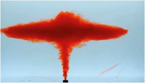
In keeping with all such averaging methods, closure of the model requires constitutive assumptions for the profile coefficients $D_G$ and $D_1$; see also Woodhouse et al. (2016). These involve the profiles for w and G. For example, a top hat assumption gives $D_G=D_1=1$. For constant values of these, the equations can be integrated analytically, to predict the rise height of a plume in a stratified medium, such as shown in figure 2.

Figure 2. The umbrella cloud resulting from a plume rising in a stratified medium. Image courtesy of Andy Woods.

2.5. Eddy viscosity

Prandtl's mixing-length theory (Prandtl 1925) was used by Schmidt (1941a,b) to prescribe the eddy diffusivity: (26) ${\nu }_T^{}=l_P^2\left|\frac{\mathrm{\partial }w}{\mathrm{\partial }r}\right|,$(26) and Schmidt chose the mixing-length $l_P\propto$ plume radius b and thus also z (since the similarity solution has $b\propto z$). As Schlichting (1979) comments, this choice is unsatisfactory away from boundaries, insofar as it predicts zero eddy diffusivity in the middle of the plume. On the other hand, it works very well near rigid boundaries, where it can predict the logarithmic layer for example. Prandtl (1942) suggested a simpler assumption for ‘free’ turbulence (away from walls) which in the present case we could write as (27) ${\nu }_T^{}={ϵ}_T^{}\overline{w}b,$(27) and this would be a better assumption if the Reynolds stresses were concentrated near the plume edge, i.e., a top hat velocity profile was appropriate. Both of the formulations (26(26) ${\nu }_T^{}=l_P^2\left|\frac{\mathrm{\partial }w}{\mathrm{\partial }r}\right|,$(26) ) and (27(27) ${\nu }_T^{}={ϵ}_T^{}\overline{w}b,$(27) ) were used in his discussion of turbulent jets by Rajaratnam (1976, chapter 2). However, the assumption that stresses are larger at the edge is not borne out by experiment (e.g., Wang and Law 2002). Here we propose to use a different choice, (28) ${\nu }_T^{}={ϵ}_T^{}wb,$(28) which is perhaps the simplest choice which is essentially consistent with both of the comments above. We should emphasise that this choice is not made because of an aim to improve model fits to experimental data. After all, Schmidt already showed in his 1941 papers that a cross-sectionally constant viscosity provided a satisfactory fit to his data. Rather, our purpose is to examine the mathematical structure of plume theory, with a particular emphasis on whether presumption of a finite plume width is appropriate, and if so, whether entrainment needs to be prescribed.

In their experiments, Wang and Law (2002) measured the turbulent fluxes, so it is possible to consider the applicability of (28(28) ${\nu }_T^{}={ϵ}_T^{}wb,$(28) ). From experiment, and defining $\eta =\frac{r}{z}$, they took velocity and Reynolds shear stress profiles (29) $\begin{array}{rl}w& =w_c\exp [-{\left(\frac{\eta }{{\eta }_w}\right)}^2],\\ -\overline{u^{\prime }{w}^{\prime }}& =-w_c^{2}A[\exp \{-k_g(\eta -{\eta }_0{)}^2\}-\exp \{-k_g(\eta +{\eta }_0{)}^2\}],\end{array}$(29) with constants ${\eta }_w=0.105$, A = 0.02084, $k_g=224.4$, ${\eta }_0=0.06815$ (see their equations (14) and (34), and tables 3 and 6). In figure 3, we plot the consequent values of ${\tau }_R^{}$, the scaled Reynolds shear stress, and ${\tau }_E^{}$, the scaled modelled Reynolds stress defined using (28(28) ${\nu }_T^{}={ϵ}_T^{}wb,$(28) ); specifically, these quantities are defined by (30) ${\tau }_R^{}=-\frac{\overline{u^{\prime }{w}^{\prime }}}{w_c^2},{\tau }_E^{}=\frac{{\nu }_T^{}}{w_c^2}\frac{\mathrm{\partial }w}{\mathrm{\partial }r},{\nu }_T^{}={ϵ}_T^{}bw,b=\text{β}z,$(30) and the values of $\text{β}=3.96$ and ${ϵ}_T^{}=0.03$ are chosen. The value of β is that which we find later in solving for the velocity and buoyancy profiles in a similarity solution appropriate when N = 0; it does not assume any particular value of the entrainment coefficient. It is of course possible to tweak these values to obtain a better fit (for example, try ${\eta }_w=0.135$ and ${ϵ}_T^{}=0.034$), but our point is that the assumption in (28(28) ${\nu }_T^{}={ϵ}_T^{}wb,$(28) ) is reasonably consistent with this set of experimental data.

Figure 3. The quantities ${\tau }_E$ and ${\tau }_R$ defined by (30(30) ${\tau }_R^{}=-\frac{\overline{u^{\prime }{w}^{\prime }}}{w_c^2},{\tau }_E^{}=\frac{{\nu }_T^{}}{w_c^2}\frac{\mathrm{\partial }w}{\mathrm{\partial }r},{\nu }_T^{}={ϵ}_T^{}bw,b=\text{β}z,$(30) ) and (29(29) $\begin{array}{rl}w& =w_c\exp [-{\left(\frac{\eta }{{\eta }_w}\right)}^2],\\ -\overline{u^{\prime }{w}^{\prime }}& =-w_c^{2}A[\exp \{-k_g(\eta -{\eta }_0{)}^2\}-\exp \{-k_g(\eta +{\eta }_0{)}^2\}],\end{array}$(29) ), with values ${\eta }_w=0.105$, A = 0.02084, $k_g=224.4$, ${\eta }_0=0.06815$, $\text{β}=3.96$ and ${ϵ}_T^{}=0.03$. (Colour online.)

2.6. Non-dimensionalisation

It seems that the question of why plumes are thin is not often addressed, if at all. To consider this we make the model (11(11a) $\begin{array}{rl}(ru{)}_r+r{w}_z& =0,\end{array}$(11a) ) dimensionless as follows: (31) $b,r\sim d,z\sim l,w\sim w^{\ast },u\sim ϵw^{\ast },N\sim \sqrt{\frac{g}{L}},G\sim \delta g,$(31) where (32) $ϵ=\frac{d}{l},$(32) and we suppose that the ambient density ${\rho }_0$ changes on a length scale L, and that the excess buoyancy $\mathrm{\Delta }\rho \sim \delta {\rho }_0$, where in keeping with the Boussinesq approximation, we assume $\delta \ll 1$. The scales d, l and $w^{\ast }$ are yet to be chosen.

Substituting these scalings into equations (11(11a) $\begin{array}{rl}(ru{)}_r+r{w}_z& =0,\end{array}$(11a) ), and using the choice of eddy viscosity in (28(28) ${\nu }_T^{}={ϵ}_T^{}wb,$(28) ), we obtain the dimensionless equations (33a) $\begin{array}{rl}(ru{)}_r+r{w}_z& =0,\end{array}$(33a) (33b) $\begin{array}{rl}(ruw{)}_r+(r{w}^2{)}_z& =\frac{\delta gl}{w^{\ast 2}}rG+\frac{{ϵ}_T^{}}{ϵ}(rbw{w}_r{)}_r,\end{array}$(33b) (33c) $\begin{array}{rl}\frac{l}{\delta L}{N}^{2}rw+(ruG{)}_r+(rwG{)}_z& =\frac{{ϵ}_T^{}}{ϵ}(rbw{G}_r{)}_r.\end{array}$(33c) Note that N is now dimensionless and $O\left(1\right)$ by definition in a stratified ambient fluid.

There are three obvious choices for the scales which follow by taking the three dimensionless constants in (33(33a) $\begin{array}{rl}(ru{)}_r+r{w}_z& =0,\end{array}$(33a) ) to be equal to one, and this determines (34) $l=\delta L,w^{\ast }=\sqrt{\delta gl},ϵ={ϵ}_T^{},d={ϵ}_T^{}l.$(34) Note that thin plume theory is thus explicitly justified if ${ϵ}_T^{}\ll 1$. The model equations (11(11a) $\begin{array}{rl}(ru{)}_r+r{w}_z& =0,\end{array}$(11a) ) take the dimensionless form (35a) $\begin{array}{rl}(ru{)}_r+r{w}_z& =0,\end{array}$(35a) (35b) $\begin{array}{rl}(ruw{)}_r+(r{w}^2{)}_z& =rG+{\left[brw{w}_r\right]}_r,\end{array}$(35b) (35c) $\begin{array}{rl}{N}^{2}rw+(ruG{)}_r+(rwG{)}_z& ={\left[brw{G}_r\right]}_r.\end{array}$(35c) There is a slight awkwardness about this if the ambient fluid is unstratified, which corresponds to the limit $L\to \mathrm{\infty }$. In that case there is no macroscopic length scale (the only length scale is that of the inlet tube radius $a_0$, but we implicitly assume $l\gg a_0$, which renders it irrelevant). As is well known, there is then a similarity solution, and thus l is arbitrary. With this understanding, we can use (35(35a) $\begin{array}{rl}(ru{)}_r+r{w}_z& =0,\end{array}$(35a) ) as is, and simply put $N^2=0$ if the ambient medium is unstratified.

It is perhaps worth pointing out that the choice $ϵ\gg {ϵ}_T^{}$ in (33(33a) $\begin{array}{rl}(ru{)}_r+r{w}_z& =0,\end{array}$(33a) ) corresponds to choosing an essentially inviscid plume as was done by Linden (2000), with boundary layers at the sides. The inviscid problem is hyperbolic, and can be solved, but the solution is very un-plume-like (it gets narrower as it rises), and we discount this possibility.

We shall consider the model (35(35a) $\begin{array}{rl}(ru{)}_r+r{w}_z& =0,\end{array}$(35a) ) in the following section. The appropriate boundary conditions which we assume are (36) $w=G=0,u=-\frac{\alpha \overline{w}}{ϵ}\mathrm{a}\mathrm{t}r=b.$(36) The last condition is the entrainment condition, included here in case it needs to be specified as an extra condition (although in the end we will find that is a consequence of the model). Note that in a stratified medium, $N^2\left(\delta z\right)$ (remember that N is now dimensionless) is a slowly varying function of height if $\delta \ll 1$. We can then generally take N to be locally constant, but we shall now suppose N = 0, corresponding to an unstratified ambient fluid.

3. The diffusive plume

When the ambient fluid is unstratified, the Brunt–Väisälä frequency N = 0, and it is well known that the plume model (35(35a) $\begin{array}{rl}(ru{)}_r+r{w}_z& =0,\end{array}$(35a) ) possesses similarity solutions of the form (37) $w=z^{-1/3}W\left(\eta \right),u=z^{-1/3}U\left(\eta \right),G=z^{-5/3}\Gamma \left(\eta \right),\eta =\frac{r}{z},b=\text{β}z,$(37) which we would expect to correspond to the far field solution away from the inlet, and generally to be appropriate for $l\gg a_0$.

Substituting (37(37) $w=z^{-1/3}W\left(\eta \right),u=z^{-1/3}U\left(\eta \right),G=z^{-5/3}\Gamma \left(\eta \right),\eta =\frac{r}{z},b=\text{β}z,$(37) ) into (35(35a) $\begin{array}{rl}(ru{)}_r+r{w}_z& =0,\end{array}$(35a) ), we find that U, W and Γ satisfy the equations (38a) $\begin{array}{rl}(\eta U{)}^{\prime }-\eta (\frac{1}{3}W+\eta W^{\prime })& =0,\end{array}$(38a) (38b) $\begin{array}{rl}U{W}^{\prime }-W(\frac{1}{3}W+\eta W^{\prime })& =\Gamma +\frac{\text{β}}{\eta }(\eta W{W}^{\prime }{)}^{\prime },\end{array}$(38b) (38c) $\begin{array}{rl}U{\Gamma }^{\prime }-W(\frac{5}{3}\Gamma +\eta {\Gamma }^{\prime })& =\frac{\text{β}}{\eta }(\eta W{\Gamma }^{\prime }{)}^{\prime },\end{array}$(38c) with boundary conditions (39) $W=\Gamma =0,U=-\frac{2\alpha }{{ϵ}_T^{}{\text{β}}^2}{\int }_0^{\text{β}}\eta W\mathrm{d}\eta \mathrm{a}\mathrm{t}\eta =\text{β}.$(39) Additionally there are symmetry conditions at $\eta =0$: (40) $U=W^{\prime }={\Gamma }^{\prime }=0\mathrm{a}\mathrm{t}\eta =0.$(40) The first of these is automatic, and indeed (38a(38a) $\begin{array}{rl}(\eta U{)}^{\prime }-\eta (\frac{1}{3}W+\eta W^{\prime })& =0,\end{array}$(38a) ) is a quadrature for U requiring no boundary condition. The two second order equations for W and Γ use the other two boundary conditions in (40(40) $U=W^{\prime }={\Gamma }^{\prime }=0\mathrm{a}\mathrm{t}\eta =0.$(40) ), as well as the two conditions at $\eta =\text{β}$. The unknown β must then apparently be determined to satisfy the entrainment condition in (39(39) $W=\Gamma =0,U=-\frac{2\alpha }{{ϵ}_T^{}{\text{β}}^2}{\int }_0^{\text{β}}\eta W\mathrm{d}\eta \mathrm{a}\mathrm{t}\eta =\text{β}.$(39) ).

A complication arises because, as is easily seen from (24c(24c) $\begin{array}{rl}\frac{\mathrm{d}B}{\mathrm{d}z}& =-N^{2}Q,\end{array}$(24c) ), the buoyancy flux (41) $B_0=2\pi {\int }_0^{b}rwG\mathrm{d}r=2\pi {\int }_0^{\text{β}}\eta W\Gamma \mathrm{d}\eta$(41) is independent of z in general (when N = 0) and must therefore be also prescribed. This is accommodated as described below.

3.1. Numerical solution strategy

Multiplying the first equation in (38(38a) $\begin{array}{rl}(\eta U{)}^{\prime }-\eta (\frac{1}{3}W+\eta W^{\prime })& =0,\end{array}$(38a) ) by Γ and adding it to η times the third equation yields a first integral, from which we can determine (42) $U=\eta W+\frac{\text{β}W{\Gamma }^{\prime }}{\Gamma },$(42) and substituting this into (38(38a) $\begin{array}{rl}(\eta U{)}^{\prime }-\eta (\frac{1}{3}W+\eta W^{\prime })& =0,\end{array}$(38a) ) yields the two equations for W and Γ: (43) $\begin{array}{rl}\frac{\text{β}W{\Gamma }^{\prime }{W}^{\prime }}{\Gamma }-\frac{1}{3}{W}^2& =\Gamma +\frac{\text{β}}{\eta }(\eta W{W}^{\prime }{)}^{\prime },\\ \frac{\text{β}W{\Gamma }^{\prime }{}^2}{\Gamma }-\frac{5}{3}W\Gamma & =\frac{\text{β}}{\eta }(\eta W{\Gamma }^{\prime }{)}^{\prime };\end{array}$(43) the entrainment condition in (39(39) $W=\Gamma =0,U=-\frac{2\alpha }{{ϵ}_T^{}{\text{β}}^2}{\int }_0^{\text{β}}\eta W\mathrm{d}\eta \mathrm{a}\mathrm{t}\eta =\text{β}.$(39) ) takes the form (44) $W^{\prime }=-\frac{2\alpha }{{ϵ}_T^{}{\text{β}}^3}{\int }_0^{\text{β}}\eta W\mathrm{d}\eta \mathrm{a}\mathrm{t}\eta =\text{β}$(44) (here we have used l'Hôpital's rule as inspection of (38(38a) $\begin{array}{rl}(\eta U{)}^{\prime }-\eta (\frac{1}{3}W+\eta W^{\prime })& =0,\end{array}$(38a) ) shows that W and Γ have finite derivatives at the plume edge). It may be convenient to rescale η by writing $\eta =\sqrt{\text{β}}\zeta$, so that (45) $\begin{array}{rl}\frac{W{\Gamma }^{\prime }{W}^{\prime }}{\Gamma }-\frac{1}{3}{W}^2& =\Gamma +\frac{1}{\zeta }(\zeta W{W}^{\prime }{)}^{\prime },\\ \frac{W{\Gamma }^{\prime }{}^2}{\Gamma }-\frac{5}{3}W\Gamma & =\frac{1}{\zeta }(\zeta W{\Gamma }^{\prime }{)}^{\prime }\end{array}$(45) (the primes now referring to ζ-derivatives), subject to the same boundary conditions: (46a) $\begin{array}{rl}{W}^{\prime }={\Gamma }^{\prime }=0& \mathrm{o}\mathrm{n}\zeta =0,\end{array}$(46a) (46b) $\begin{array}{rl}W=\Gamma =0& \mathrm{a}\mathrm{t}\zeta =\Omega =\sqrt{\text{β}},\end{array}$(46b) and the entrainment condition can then be written in the form (47) $W^{\prime }=-\frac{2\alpha }{{ϵ}_T^{}{\text{β}}^{3/2}}{\int }_0^{\Omega }\zeta W\mathrm{d}\zeta \mathrm{a}\mathrm{t}\zeta =\Omega .$(47) We need to deal with the buoyancy flux constraint (41(41) $B_0=2\pi {\int }_0^{b}rwG\mathrm{d}r=2\pi {\int }_0^{\text{β}}\eta W\Gamma \mathrm{d}\eta$(41) ), not to mention the fact that $W=\Gamma =0$ is a perfectly adequate solution of (45(45) $\begin{array}{rl}\frac{W{\Gamma }^{\prime }{W}^{\prime }}{\Gamma }-\frac{1}{3}{W}^2& =\Gamma +\frac{1}{\zeta }(\zeta W{W}^{\prime }{)}^{\prime },\\ \frac{W{\Gamma }^{\prime }{}^2}{\Gamma }-\frac{5}{3}W\Gamma & =\frac{1}{\zeta }(\zeta W{\Gamma }^{\prime }{)}^{\prime }\end{array}$(45) ). In fact equations (45(45) $\begin{array}{rl}\frac{W{\Gamma }^{\prime }{W}^{\prime }}{\Gamma }-\frac{1}{3}{W}^2& =\Gamma +\frac{1}{\zeta }(\zeta W{W}^{\prime }{)}^{\prime },\\ \frac{W{\Gamma }^{\prime }{}^2}{\Gamma }-\frac{5}{3}W\Gamma & =\frac{1}{\zeta }(\zeta W{\Gamma }^{\prime }{)}^{\prime }\end{array}$(45) ) are invariant under the re-scaling $W\sim \lambda$, $\Gamma \sim {\lambda }^2$, and so there is a one-parameter family of solutions, and then (41(41) $B_0=2\pi {\int }_0^{b}rwG\mathrm{d}r=2\pi {\int }_0^{\text{β}}\eta W\Gamma \mathrm{d}\eta$(41) ) provides the normalisation to select the unique solution. Equations (45(45) $\begin{array}{rl}\frac{W{\Gamma }^{\prime }{W}^{\prime }}{\Gamma }-\frac{1}{3}{W}^2& =\Gamma +\frac{1}{\zeta }(\zeta W{W}^{\prime }{)}^{\prime },\\ \frac{W{\Gamma }^{\prime }{}^2}{\Gamma }-\frac{5}{3}W\Gamma & =\frac{1}{\zeta }(\zeta W{\Gamma }^{\prime }{)}^{\prime }\end{array}$(45) ) can be rewritten in the form (48) $\begin{array}{rl}{\left(\frac{\zeta W{W}^{\prime }}{\Gamma }\right)}^{\prime }& =-\zeta (1+\frac{W^2}{3\Gamma }),\\ {\left(\frac{\zeta W{\Gamma }^{\prime }}{\Gamma }\right)}^{\prime }& =-\frac{5}{3}\zeta W.\end{array}$(48) The two equations in (48(48) $\begin{array}{rl}{\left(\frac{\zeta W{W}^{\prime }}{\Gamma }\right)}^{\prime }& =-\zeta (1+\frac{W^2}{3\Gamma }),\\ {\left(\frac{\zeta W{\Gamma }^{\prime }}{\Gamma }\right)}^{\prime }& =-\frac{5}{3}\zeta W.\end{array}$(48) ) can be written as the two pairs (49) $\zeta W^{\prime }=-\frac{\Gamma P}{W},P^{\prime }=\zeta (1+\frac{W^2}{3\Gamma }),$(49) which are to be solved (given Γ) with boundary conditions (50) $P=0\mathrm{a}\mathrm{t}\zeta =0,W=0\mathrm{a}\mathrm{t}\zeta =\Omega$(50) and (51) $\zeta W{\Gamma }^{\prime }=-\Gamma Q,Q^{\prime }=\frac{5}{3}\zeta W,$(51) which are to be solved (given W) subject to the boundary conditions (52) $Q=0\mathrm{a}\mathrm{t}\zeta =0,\Gamma =0\mathrm{a}\mathrm{t}\zeta =\Omega .$(52)

3.1.1. Local expansions

We assume near $\zeta =0$ that (53) $W\approx W_0-W_2{\zeta }^2,\Gamma \approx {\Gamma }_0-{\Gamma }_2{\zeta }^2,P\approx P_2{\zeta }^2,Q\approx Q_2{\zeta }^2.$(53) Substituting these into (49(49) $\zeta W^{\prime }=-\frac{\Gamma P}{W},P^{\prime }=\zeta (1+\frac{W^2}{3\Gamma }),$(49) ) and (51(51) $\zeta W{\Gamma }^{\prime }=-\Gamma Q,Q^{\prime }=\frac{5}{3}\zeta W,$(51) ), we find the results are self-consistent, and in particular (54) $\Gamma \sim {\Gamma }_0(1-\frac{5}{12}{\zeta }^2)\mathrm{a}\mathrm{s}\zeta \to 0.$(54) Near $\zeta =\Omega$, we suppose (55) $W\sim W_1(\Omega -\zeta ),\Gamma \sim {\Gamma }_1(\Omega -\zeta ),P\sim P_1>0,Q\sim Q_1>0,$(55) and these are also consistent, but importantly, ${\Gamma }_1$ is unconstrained. In particular, the first equation in (51(51) $\zeta W{\Gamma }^{\prime }=-\Gamma Q,Q^{\prime }=\frac{5}{3}\zeta W,$(51) ) implies that (56) $Q=-\Omega W^{\prime }\mathrm{a}\mathrm{t}\zeta =\Omega .$(56) Using (51(51) $\zeta W{\Gamma }^{\prime }=-\Gamma Q,Q^{\prime }=\frac{5}{3}\zeta W,$(51) ), (52(52) $Q=0\mathrm{a}\mathrm{t}\zeta =0,\Gamma =0\mathrm{a}\mathrm{t}\zeta =\Omega .$(52) ) and (56(56) $Q=-\Omega W^{\prime }\mathrm{a}\mathrm{t}\zeta =\Omega .$(56) ), the entrainment condition simply implies that Ω is actually determined as (57) $\Omega ={\left(\frac{6\alpha }{5{ϵ}_T^{}}\right)}^{1/2},$(57) in view of (46(46a) $\begin{array}{rl}{W}^{\prime }={\Gamma }^{\prime }=0& \mathrm{o}\mathrm{n}\zeta =0,\end{array}$(46a) ). We emphasise the significance of this. If the entrainment condition is applied, then it determines the location of the plume edge; or, if the plume edge is determined independently from the solution of (58(58a) $\begin{array}{rl}{W}^{\prime }=-\frac{\Gamma P}{2xW},& P^{\prime }=\frac{1}{2}(1+\frac{W^2}{3\Gamma }),\end{array}$(58a) ) and (59(59) $P=Q=0\mathrm{a}\mathrm{t}x=0,\Gamma =W=0\mathrm{a}\mathrm{t}x=\text{β}=\frac{6\alpha }{5{ϵ}_T^{}}.$(59) ) below, then it implies the entrainment condition, and also the value of the entrainment coefficient.

3.1.2. Entrainment

It is mildly convenient to define $x={\zeta }^2$, so that (49(49) $\zeta W^{\prime }=-\frac{\Gamma P}{W},P^{\prime }=\zeta (1+\frac{W^2}{3\Gamma }),$(49) ) and (51(51) $\zeta W{\Gamma }^{\prime }=-\Gamma Q,Q^{\prime }=\frac{5}{3}\zeta W,$(51) ) have the form (58a) $\begin{array}{rl}{W}^{\prime }=-\frac{\Gamma P}{2xW},& P^{\prime }=\frac{1}{2}(1+\frac{W^2}{3\Gamma }),\end{array}$(58a) (58b) $\begin{array}{rl}{\Gamma }^{\prime }=-\frac{\Gamma Q}{2xW},& Q^{\prime }=\frac{5}{6}W,\end{array}$(58b) where the primes now denote differentiation with respect to x. The boundary conditions are (59) $P=Q=0\mathrm{a}\mathrm{t}x=0,\Gamma =W=0\mathrm{a}\mathrm{t}x=\text{β}=\frac{6\alpha }{5{ϵ}_T^{}}.$(59) It is not difficult to show that the variables have regular Taylor expansions about x = 0. Now since the equations are invariant under the scaling $W\sim \lambda$, $\Gamma \sim {\lambda }^2$, $Q\sim \lambda$, $P\sim 1$, the value of $\Gamma ={\Gamma }_0$ can be chosen arbitrarily, and its actual value is then fixed by the buoyancy flux $B_0$. That is to say, solve the problem with ${\Gamma }_0=1$, say; then under the re-scaling above, the solution is obtained by choosing λ so that (41(41) $B_0=2\pi {\int }_0^{b}rwG\mathrm{d}r=2\pi {\int }_0^{\text{β}}\eta W\Gamma \mathrm{d}\eta$(41) ) is satisfied.

This implies that if we solve (58(58a) $\begin{array}{rl}{W}^{\prime }=-\frac{\Gamma P}{2xW},& P^{\prime }=\frac{1}{2}(1+\frac{W^2}{3\Gamma }),\end{array}$(58a) ) as an initial value problem with ${\Gamma }_0=1$, the only quantity which can be varied is the value of $W=W_0$ at x = 0; but $W_0$ must be chosen to satisfy the two boundary conditions at $x=\text{β}$. These appear to be independent, which implies that β must be chosen in order to enable this. The apparent implication is that the entrainment condition, at least in this formulation of the model, is actually a consequence of the choice of eddy viscosity. To see whether this is so, we must solve the problem numerically.

One possibility is to use a shooting method, as indicated above. This is not generally advisable for boundary value problems, and a suitable iterative scheme would be more natural. However, the constraint in (56(56) $Q=-\Omega W^{\prime }\mathrm{a}\mathrm{t}\zeta =\Omega .$(56) ) makes it difficult to see how to do this. In fact, shooting works well. Equation (58(58a) $\begin{array}{rl}{W}^{\prime }=-\frac{\Gamma P}{2xW},& P^{\prime }=\frac{1}{2}(1+\frac{W^2}{3\Gamma }),\end{array}$(58a) ) has in general two possible behaviours, subject to the initial conditions (60) $P=Q=0,\Gamma =1,W=W_0\mathrm{a}\mathrm{t}x=0;$(60) these are that $W\to 0$ at finite x, with a square root singularity if $\Gamma >0$; or $\Gamma \sim e^{-\frac{2}{3}x}$, $W\sim x^{-1/4}$ as $x\to \mathrm{\infty }$. The first behaviour is found for sufficiently small $W_0<W_c$, and the second for $W_0>W_c$. At the unique value $W_c\approx 1.02$, W and Γ both reach zero (linearly) at a value $x=\text{β}\approx 3.96$, and thus $\zeta =\sqrt{\text{β}}\approx 1.99$. 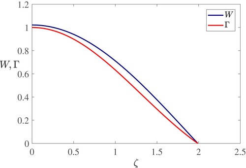Care is needed because of the potential singular behaviour at both end points. Figure 4 shows the solutions for W and Γ computed at the critical values. Because β is determined independently of the entrainment condition, it follows that the entrainment condition is not an independent constraint, but is determined by the model, and (57(57) $\Omega ={\left(\frac{6\alpha }{5{ϵ}_T^{}}\right)}^{1/2},$(57) ) determines the value of α.

Figure 4. Computed profiles of W (upper curve) and Γ (lower curve). The values of $W_0$ and β are 1.0217 and 3.9612 respectively in this calculation. (Colour online.)

3.1.3. Taylor series expansion

Equations (58(58a) $\begin{array}{rl}{W}^{\prime }=-\frac{\Gamma P}{2xW},& P^{\prime }=\frac{1}{2}(1+\frac{W^2}{3\Gamma }),\end{array}$(58a) ) have regular Taylor series expansions of the form (61a) $\begin{array}{rl}\Gamma & =1+g_{1}x+g_2{x}^2+\cdots ,\end{array}$(61a) (61b) $\begin{array}{rl}W& =W_0[1+w_{1}x+w_2{x}^2+\cdots ],\end{array}$(61b) (61c) $\begin{array}{rl}P& =W_0^2[p_{1}x+p_2{x}^2+\cdots ],\end{array}$(61c) (61d) $\begin{array}{rl}Q& =W_0[q_{1}x+q_2{x}^2+\cdots ],\end{array}$(61d) and the first few coefficients are given in table 1 for the particular choice $W_0=1.0217$. These approximations are useful in checking the numerical solution. Calculation of the coefficients can be enabled automatically through the iteration scheme for $n\ge 0$, (62a) $\begin{array}{rl}{q}_{n+1}& =\frac{5w_n}{6(n+1)},\end{array}$(62a) (62b) $\begin{array}{rl}{g}_{n+1}& =\frac{1}{n+1}[-\frac{1}{2}\{q_{n+1}+\sum _{j=0}^{n-1}{g}_{j+1}{q}_{n-j}\}-\sum _{j=0}^{n-1}(j+1\left)g_{j+1}{w}_{n-j}\right],\end{array}$(62b) (62c) $\begin{array}{rl}{p}_{n+1}& =\frac{1}{n+1}[\mu g_n+\frac{1}{6}\sum _{j=0}^n{w}_j{w}_{n-j}-\sum _{j=1}^{n}j{p}_j{g}_{n-j+1}],\end{array}$(62c) (62d) $\begin{array}{rl}{w}_{n+1}& =\frac{1}{n+1}[-\frac{1}{2}\{p_{n+1}+\sum _{j=1}^n{g}_j{p}_{n-j+1}\}-\sum _{j=1}^{n}j{w}_j{w}_{n-j+1}],\end{array}$(62d) in which (63) $w_0=1,g_0=1,\mu =\frac{1}{2W_0^2}.$(63)

Table 1. Coefficients in the Taylor expansions in (61(61a) $\begin{array}{rl}\Gamma & =1+g_{1}x+g_2{x}^2+\cdots ,\end{array}$(61a) ) for a value $W_0=1.0217$.

n	$g_n$	$w_n$	$p_n$	$q_n$
1	$-0.416667$	$-0.322827$	0.645653	0.833333
2	$0.531778\times {10}^{-1}$	$0.199176\times {10}^{-1}$	$-0.190822\times {10}^{-1}$	$-0.134511$
3	$-0.343783\times {10}^{-2}$	$-0.575621\times {10}^{-3}$	$-0.252036\times {10}^{-3}$	$0.553266\times {10}^{-2}$
4	$0.133468\times {10}^{-3}$	$0.848386\times {10}^{-5}$	$-0.119393\times {10}^{-4}$	$-0.119921\times {10}^{-3}$
5	$-0.341983\times {10}^{-5}$	$-0.859618\times {10}^{-7}$	$-0.449965\times {10}^{-6}$	$0.141398\times {10}^{-5}$
6	$0.620654\times {10}^{-7}$	$0.266417\times {10}^{-9}$	$-0.161194\times {10}^{-7}$	$-0.119391\times {10}^{-7}$
7	$-0.923082\times {10}^{-9}$	$-0.101864\times {10}^{-9}$	$-0.556292\times {10}^{-9}$	$0.317163\times {10}^{-10}$
8	$-0.630841\times {10}^{-11}$	$-0.229750\times {10}^{-10}$	$-0.205264\times {10}^{-10}$	$-0.106108\times {10}^{-10}$
9	$-0.348262\times {10}^{-11}$	$-0.516569\times {10}^{-11}$	$-0.117409\times {10}^{-11}$	$-0.212732\times {10}^{-11}$
10	$-0.773856\times {10}^{-12}$	$-0.117037\times {10}^{-11}$	$-0.145728\times {10}^{-12}$	$-0.430474\times {10}^{-12}$

3.2. Comparison with experiment

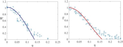
As much of our introductory discussion focusses on the work of Schmidt (1941a,b) and Rouse et al. (1952), we first compare our theory with their results. Both sets of experiments used hot air as the plume fluid. They provided profiles of velocity and buoyancy across the plume in terms of the similarity scaling, and can thus be directly compared with our similarity solutions. Schmidt provided measurements of root mean square velocity (which is in any case close to the mean vertical velocity) whereas Rouse et al. gave just the vertical velocity. Rouse et al. fit Gaussians to their data, and the use of Gaussians for plume variation is now an acquired habit (e.g., Turner 1973), whereas Schmidt fit his calculated Frobenius series for his model, which worked equally well.

In figures 5 and 6, we compare these experimental results with the predictions from our model. As we choose to normalise the data so that the maximum of each curve is one, all that is really being compared here is the overall shape and the width, which depends on ${ϵ}_T^{}$.

Figure 5. Comparison of the similarity solution with the Schmidt (1941b) data, using a value ${ϵ}_T^{}=0.0505$. (Colour online.)

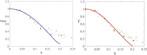
Figure 6. Comparison of the similarity solution with the Rouse et al. (1952) data, using values ${ϵ}_T^{}=0.0341$ (left) and ${ϵ}_T^{}=0.0404$ (right). (Colour online.)

Due to improvements in the accuracy of experimental procedure in more modern times, as well as the introduction of direct numerical simulation (DNS) data, we also include in figure 7 a comparison to the experimental data of Ezzamel et al. (2015) and Shabbir and George (1994), as well as the DNS data of Marjanovic et al. (2017) (at z = 15) and van Reeuwijk et al. (2016). All of these works provide profiles of velocity and buoyancy across the plume in terms of a similarity scaling and we normalise and scale to the same width. For Marjanovic et al. (2017), we consider the case in which the plume is only slightly lazy, when the plume source parameter in their notation ${\Gamma }_0=0.75\sqrt{2}$, where ${\Gamma }_0=1$ represents a pure plume, ${\Gamma }_0<1$ a forced plume or buoyant jet (excess of momentum) and ${\Gamma }_0>1$ a lazy plume (deficit of momentum flux) (see also Morton 1959, Morton and Middleton 1973, Hunt and Kaye 2001, Hunt and Van Den Bremer 2011). For the DNS data of van Reeuwijk et al. (2016), we just look at a few points from along the velocity and buoyancy curves of their similarity profiles. Later we will also add a further comparison with the results of Burridge et al. (2017).

Figure 7. Comparison of the similarity solution with the data of Ezzamel et al. (2015) (ESH), Shabbir and George (1994) (SG), Marjanovic et al. (2017) (MTB) and van Reeuwijk et al. (2016) (RSHC). We have normalised all data to the same height and made all the same width, which required scaling the width of Ezzamel et al. (2015) and van Reeuwijk et al. (2016) both of which are given in terms of $\frac{r}{b}$ rather than $\frac{r}{z}$, this was done using a value of ${ϵ}_T^{}=0.0454$ with $\text{β}=3.9612$. (Colour online.)

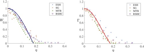
We see that away from the plume edge, the shapes are reasonably well fit, with values of ${ϵ}_T^{}\sim 0.03$ – 0.05. We note from (59(59) $P=Q=0\mathrm{a}\mathrm{t}x=0,\Gamma =W=0\mathrm{a}\mathrm{t}x=\text{β}=\frac{6\alpha }{5{ϵ}_T^{}}.$(59) ) that the entrainment coefficient is defined by (64) $\alpha =\frac{5}{6}{ϵ}_T^{}\text{β},$(64) and since our numerical solution determines $\text{β}=3.96$, this range of ${ϵ}_T^{}$ corresponds to values of α in the range 0.1–0.17, in good agreement with values determined experimentally (Carazzo et al. 2006).

The most obvious discrepancy between the data and the experiments lies in the tails at the plume edge, which indeed are more Gaussian than abrupt. From the point of view of the Schmidt theory, the simplest explanation is that our choice of eddy viscosity is wrong, and a more nearly cross-sectionally constant value such as that used by Schmidt is appropriate. The problem with this is that figure 1 is clearly suggestive of a precisely defined average plume width. Furthermore, as we discuss in the following section, the derivation of the usual moment equations does rely implicitly on the assumptions of the boundary conditions at the plume edge.

One comment of relevance may be the following. Although the mean plume edge $\eta =\overline{\text{β}}$ (see (37(37) $w=z^{-1/3}W\left(\eta \right),u=z^{-1/3}U\left(\eta \right),G=z^{-5/3}\Gamma \left(\eta \right),\eta =\frac{r}{z},b=\text{β}z,$(37) )) may be constant, the actual plume edge $\eta =\text{β}$ fairly obviously fluctuates (see figure 1). Detailed experiments by Burridge et al. (2017) show that the plume edge is well approximated by a Gaussian distribution, suggesting that it could be described by an essentially statistical process. What is the effect of this on the mean velocity profile? Let us give a simple example, in which we take a top hat profile w = 1 for $\eta <\text{β}$, w = 0 for $\eta >\text{β}$ and suppose that β has a probability density $\varphi \left(\eta \right)$ with respect to the radial variable η. Then (65) $P(w=1)=P(\text{β}>\eta )={\int }_{\eta }^{\mathrm{\infty }}\varphi \left(y\right)\mathrm{d}y,$(65) and this is also the distribution of the mean velocity. For example, a Gaussian mean velocity $w=e^{-{\eta }^2/{\eta }_0^2}$ follows from the choice (66) $\varphi =\frac{2\eta }{{\eta }_0^2}{e}^{-{\eta }^2/{\eta }_0^2}.$(66) The point is that plume boundary fluctuations will cause a smoothing of the mean velocity profile, although it is less obvious how to deal with this in the context of the Schmidt theory.

4. Discussion

The Schmidt (1941a,b) model of plume dynamics, in which Reynolds stresses and turbulent buoyancy transport are modelled by eddy diffusive terms, has been to a large extent superseded by the retention of the original quadratic fluctuation average terms, and the use of integral moments to provide a reduced set of ordinary differential equations for the moments of mass flux, momentum flux, buoyancy flux and, in the case of Priestley and Ball (1955) and others, kinetic energy flux.

There is thus a dichotomy in the evolution of plume models, depending on whether closures for the eddy transport terms are provided or not. If not, integral moment theories are necessary, and the closures then take the form of assuming cross-sectional profiles, commonly chosen as Gaussian, so that a closed system can be formed for the moments. However, there is no unique way of doing this, because one can form an infinite number of different moment equations. Already this discrepancy is seen in the comparison between the theories of Priestley and Ball (1955) and Morton et al. (1956).

A further dichotomy in the models lies in whether the plume is taken to be of finite width or infinite width. Visibly, plumes are finite (Burridge et al. 2017), but measured velocity and buoyancy profiles, being apparently Gaussian, suggest that the plume can be taken to extend to infinity. In this case plume ‘width’ b can be taken as a measure of the width of the Gaussian. For example, we might define the vertical velocity as measured to be (67) $w=w_c\exp (-r^2/b^2);$(67) or we might define the width via an equivalent top hat profile: (68) $w_{c}b={\int }_0^{\mathrm{\infty }}w\mathrm{d}r.$(68) In either case, entrainment occurs at the plume edge: mass conservation implies that (see (16(16) $\frac{\mathrm{d}}{\mathrm{d}z}{\int }_0^{\mathrm{\infty }}rw\mathrm{d}r=-{\left(ru\right)|}_{\mathrm{\infty }}=\alpha b{w}_0$(16) )) (69) $\frac{\mathrm{d}}{\mathrm{d}z}{\int }_0^{b}rw\mathrm{d}r=-{\left(ru\right)|}_b,$(69) whether b is finite or infinite. Taking the plume width to be finite, Morton et al. (1956) then had to prescribe the entrainment rate as a boundary condition on u at b. On the other hand, if the plume is infinite, Fox (1970) suggests that the entrainment rate can be determined through the integral moment equations.

From the point of view of a mathematical model, this raises the question as to whether the finite and infinite plume models are fundamentally different, in terms of whether entrainment is prescribed or not. We think that this question can only be sensibly answered if turbulent closures are specified, for then the model becomes a closed system of partial differential equations with associated boundary conditions.

Supposing that an eddy viscosity model is a suitable closure, and that the corresponding model is given by (11(11a) $\begin{array}{rl}(ru{)}_r+r{w}_z& =0,\end{array}$(11a) ), then an infinite plume model is associated with a non-zero value of the (eddy) viscosity ${\nu }_T^{}$ everywhere, including in the far field, where one would suppose the laminar molecular value ${\nu }_L^{}$ (the kinematic viscosity) would be appropriate, i.e. ${\nu }_T^{}\to {\nu }_L^{}$ as $r\to \mathrm{\infty }$. In this case the boundary conditions for (11(11a) $\begin{array}{rl}(ru{)}_r+r{w}_z& =0,\end{array}$(11a) ) are simply w = G = 0 at $r=\mathrm{\infty }$, and the entrainment condition is presumably a consequence of the asymptotic behaviour of u at ∞, since u is obtained by quadrature as (70) $u=-\frac{1}{r}{\int }_0^{r}r{w}_z\mathrm{d}r.$(70) This is what underlies Fox's (1970) pragmatic determination of the entrainment coefficient from the moments derived from experimental data.

Now in practice the far field (kinematic) viscosity is very small. For Burridge et al.'s (2017) experiments, and using a value of ${ϵ}_T^{}\sim 0.03$ in (27(27) ${\nu }_T^{}={ϵ}_T^{}\overline{w}b,$(27) ) or (28(28) ${\nu }_T^{}={ϵ}_T^{}wb,$(28) ), we find from their table 1 that ${\nu }_T^{}/{\nu }_L^{}$ is in the range 80–150. From their figure 5, we see that edge fluctuations are essentially absent at radial distance $r\approx 2b$. This suggests that the value of ${\nu }_T^{}$ in the plume should effectively decrease to zero at the plume edge, and the simplest way to do this is to have it vanish when w = 0. The choice we have made here in (28(28) ${\nu }_T^{}={ϵ}_T^{}wb,$(28) ) is the simplest such choice, but others are possible.

Now the consequence of this is that the diffusion coefficients in (11(11a) $\begin{array}{rl}(ru{)}_r+r{w}_z& =0,\end{array}$(11a) ) are degenerate, and as a result, the prescription of boundary conditions at what is now a free boundary are less than clear. We continue to require w = G = 0 there, but one might expect an extra condition to be required to determine the plume boundary, and the natural candidate would be the entrainment condition, which would then need to be prescribed rather than deduced. In particular, the choice of a non-vanishing eddy viscosity such as that used by Schmidt (1941a,b), together with the assumption of a finite width plume, would require such an extra condition.

However, what we find, by consideration of the similarity form which is appropriate for an unstratified ambient medium, is that in fact the degeneracy of the model with vanishing eddy viscosity at the margin also predicts the entrainment condition, and specifically in the form (15(15) $u=-u_e=-\alpha \overline{w}\mathrm{a}\mathrm{t}r=b,$(15) ), and it also gives an explicit value for the entrainment coefficient α via (57(57) $\Omega ={\left(\frac{6\alpha }{5{ϵ}_T^{}}\right)}^{1/2},$(57) ) as (71) $\alpha =\frac{5}{6}{ϵ}_T^{}\text{β}\approx \frac{10}{3}{ϵ}_T^{},$(71) with apparent estimates of ${ϵ}_T^{}\sim 0.03$–0.05 giving $\alpha \sim 0.1$–0.17, which is in line with experimental results (Carazzo et al. 2006). We emphasise that this is a deduction from the solution of the point forms of the equations, and does not rely on any presumed profiles of the variables. For an eddy viscosity which vanishes at the plume edge, entrainment is a consequence of the describing equations, just as it is for the infinite plume with non-vanishing viscosity.

However, while our results may illuminate the classical Morton–Taylor–Turner theory of finite width plumes, they seem to lose ground in comparison of our predicted velocity profiles with experimental data, principally because of the lack of a Gaussian tail. Figures 5–7 showed this explicitly for various sets of experimental data. One comment worth making is that both the Rouse et al. (1952) and Schmidt (1941a,b) experiments were made in air, which at ${20}^{\circ }$C has a kinematic viscosity 15 times higher than water. We might then expect the ratio ${\nu }_T^{}/{\nu }_L^{}$ to be in the range 5–10, and given the square root dependence of diffusional profiles on the diffusion coefficient, the explanation may simply be in retaining a finite value of ${\nu }_T^{}$ to $r=\mathrm{\infty }$ (and thus an infinite plume).

Pursuing this concept suggests the idea of studying the model (35(35a) $\begin{array}{rl}(ru{)}_r+r{w}_z& =0,\end{array}$(35a) ), except that we choose the dimensionless viscosity to be $\nu +bw$, rather than bw, where, following (34(34) $l=\delta L,w^{\ast }=\sqrt{\delta gl},ϵ={ϵ}_T^{},d={ϵ}_T^{}l.$(34) ), we choose (72) $\nu =\frac{{\nu }_L^{}}{{ϵ}_T^{}{w}^{\ast }d}=\frac{{\nu }_L^{}}{{ϵ}_T^{}{}^2\sqrt{\delta g{l}^3}}.$(72) If $\nu \ll 1$, then the leading order solution is that we have given for a finite plume, but this approximation breaks down as $w\to 0$, and we expect then to pick up the Gaussian tail. A probable way to construct such an improved approximation is by using the method of strained coordinates, but such exploration awaits future work. It seems possible that such an approach could be used in comparison with experimental data, in much the same way as the integral moment method has been used (e.g., van Reeuwijk and Craske 2015, van Reeuwijk et al. 2016).

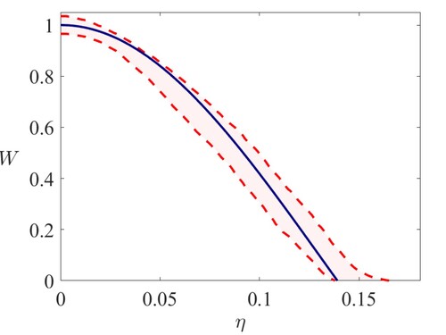
We find an intriguing comparison in the experiments of Burridge et al. (2017). These experiments were done with aqueous solutions, and the velocity measurements were also filtered to separate them into ‘eddy-present’ and ‘eddy-absent’ components; figure 8 shows a comparison of our predicted velocity profile with the eddy-present measurements. The broader spread of the actual mean velocity profile (not shown) is associated with the eddy-absent velocity profile which roughly corresponds to measurements in the ambient fluid as it is being entrained into the plume. It is noticeable that the eddy-present velocity appears to truncate at finite distance. It represents situations when there is almost no vertical motion outside the plume (which corresponds to our assumption).

Figure 8. Comparison of our predicted velocity profile with the eddy-present velocity profiles of Burridge et al. (2017, figure 13, and making use of values from their table 1). The two dashed lines indicate the range of experimental profiles. To obtain this fit we use a value ${ϵ}_T^{}=0.0351$. (Colour online.)

In our analysis, we have focussed on the case of an unstratified ambient medium, but there seems to be nothing in the formulation for a stratified medium that would give different results. That is, we would expect similar cross-sectional profile behaviour, with zero Reynolds stress at the plume edge, and that an entrainment condition would occur naturally as a consequence.

5. Conclusions

In this paper, we have studied the mathematical structure of plume theory from the perspective of the point forms of the equations as originally given by Schmidt (1941a,b) in which the turbulent mixing terms are described by eddy diffusion. We have been particularly interested in the distinction between descriptions in which the plume is taken to have finite or infinite width, since in the latter case, the entrainment condition is presumably a consequence of the solution, whereas in the former, it seems that it must be prescribed.

Supposing that the average vertical velocity $w\to 0$ at the edge of the plume, it is natural to suggest that the eddy diffusivity will tend to zero there too, and we proposed a simple choice for this (${ϵ}_T^{}bw$, where b is plume radius) which satisfies this constraint. The mathematical consequence of this is that the resulting advection–diffusion equations are degenerate at the plume edge, since the diffusion coefficient goes to zero there; in consequence, as in nonlinear diffusion equations such as the porous medium equation (13(13) $c_t=(c{c}_x{)}_x,$(13) ), the plume is finite as a consequence of the model, but crucially, the entrainment condition is still a consequence of the solution. Further, the explicit calculation of the entrainment coefficient α in terms of the friction coefficient ${ϵ}_T^{}$ in (71(71) $\alpha =\frac{5}{6}{ϵ}_T^{}\text{β}\approx \frac{10}{3}{ϵ}_T^{},$(71) ) agrees with values obtained from experiment using the Fox integral moment method (van Reeuwijk and Craske 2015).

Where this theory appears inadequate is that it does not display the Gaussian tail of the velocity and buoyancy profiles which are experimentally measured. One possible resolution lies in how one should implement an averaged boundary condition at a fluctuating boundary, but a simpler remedy is the suggestion that the laminar viscosity of the ambient fluid should not be discounted, so that we choose an eddy viscosity of the form (73) ${\nu }_T^{}={\nu }_L^{}+{ϵ}_T^{}bw,$(73) where ${\nu }_L^{}$ is the laminar kinematic viscosity. When the laminar viscosity ${\nu }_L^{}$ is small, we regain the present theory, but it will be subject to a correction at the plume edge which we conjecture will enable the Gaussian tail to be obtained in the solution.

Disclosure statement

No potential conflict of interest was reported by the authors.

Additional information

Funding

This publication has emanated from research conducted with the financial support of Science Foundation Ireland under Grant number 18/CRT/6049. For the purpose of Open Access, the author has applied a CC BY public copyright licence to any Author Accepted Manuscript version arising from this submission.

Notes

1 The reference, a war time report for the U. S. Atomic Energy Commission, is easily available on the web, and is marked as unclassified on 2 March 1956 by W. F. Carrall; Morton et al.'s (1956) paper was published on 24 January of that year! The work is dated 16 March 1945, and treats “the dynamics of a ball of fire produced in a large explosion”. The atomic bomb was dropped on Hiroshima on 6 August of that year. The abstract (not written by Taylor) states that “the column should rise to a maximum height and then mushroom out”.

2 The usual notation is $g^{\prime }$ for reduced gravity; this is avoided here, immediately because we use primes to denote turbulent fluctuations, and later because we use primes to denote ordinary derivatives.

References

- Agrawal, A. and Prasad, A.K., Integral solution for the mean flow profiles of turbulent jets, plumes, and wakes. J. Fluids Eng. 2003, 125, 813–822.
- Batchelor, G.K., Heat convection and buoyancy effects in fluids. Quart. J. Roy. Meteorol. Soc. 1954, 80, 339–358.
- Burridge, H.C., Parker, D.A., Kruger, E.S., Partridge, J.L. and Linden, P.F., Conditional sampling of a high Péclet number turbulent plume and the implications for entrainment. J. Fluid Mech. 2017, 823, 26–56.
- Carazzo, G., Kaminski, E. and Tait, S., The route to self-similarity in turbulent jets and plumes. J. Fluid Mech. 2006, 547, 137–148.
- Caulfield, C.C.P. and Woods, A.W., Plumes with non-monotonic mixing behaviour. Geophys. Astrophys. Fluid Dyn. 1995, 79, 173–199.
- Craske, J. and Van Reeuwijk, M., Generalised unsteady plume theory. J. Fluid Mech. 2016, 792, 1013–1052.
- Delichatsios, M.A., Time similarity analysis of unsteady buoyant plumes in neutral surroundings. J. Fluid Mech. 1979, 93, 241–250.
- Drew, D.A. and Passman, S.L., Theory of Multicomponent Fluids, 1999 (Springer-Verlag: New York).
- Ezzamel, A., Salizzoni, P. and Hunt, G.R., Dynamical variability of axisymmetric buoyant plumes. J. Fluid Mech. 2015, 765, 576–611.
- Farrugia, P.S. and Micallef, A., Series solutions for turbulent plumes evolving in a natural environment. J. Eng. Thermophys. 2014, 23, 236–255.
- Fowler, A.C., Mathematical Models in the Applied Sciences, 1997 (C. U. P.: Cambridge).
- Fox, D.G., Forced plume in a stratified fluid. J. Geophys. Res. 1970, 75, 6818–6835.
- Hunt, G.R. and Kaye, N.G., Virtual origin correction for lazy turbulent plumes. J. Fluid Mech. 2001, 435, 377–396.
- Hunt, G.R. and Van Den Bremer, T.S., Classical plume theory: 1937-2010 and beyond. IMA J. Appl. Math. 2011, 76, 424–448.
- Kaminski, E., Tait, S. and Carazzo, G., Turbulent entrainment in jets with arbitrary buoyancy. J. Fluid Mech. 2005, 526, 361–376.
- Linden, P.F., Convection in the environment. In Perspectives in Fluid Dynamics: A Collective Introduction to Current Research, edited by G. K. Batchelor, M. H.K. and W. M.G., pp. 289–345, 2000 (C. U. P.: Cambridge).
- Marjanovic, G., Taub, G.N. and Balachandar, S., On the evolution of the plume function and entrainment in the near-source region of lazy plumes. J. Fluid Mech. 2017, 830, 736–759.
- Marjanovic, G., Taub, G. and Balachandar, S., On the effects of buoyancy on higher order moments in lazy plumes. J. Turbul. 2019, 20, 121–146.
- Middleton, J.H., The asymptotic behaviour of a starting plume. J. Fluid Mech. 1975, 72, 753–771.
- Morton, B.R., Forced plumes. J. Fluid Mech. 1959, 5, 151–163.
- Morton, B.R., The choice of conservation equations for plume models. J. Geophys. Res. 1971, 76, 7409–7416.
- Morton, B.R. and Middleton, J., Scale diagrams for forced plumes. J. Fluid Mech. 1973, 58, 165–176.
- Morton, B.R., Taylor, G.I. and Turner, J.S., Turbulent gravitational convection from maintained and instantaneous sources. Proc. R. Soc. Lond. A. Math. Phys. Sci. 1956, 234, 1–23.
- Prandtl, L., 7. Bericht über Untersuchungen zur ausgebildeten Turbulenz. Z. Angew. Math. Mech. 1925, 5, 136–139.
- Prandtl, L., Bemerkungen zur theorie der freien Turbulenz. Z. Angew. Math. Mech. 1942, 22, 241–243.
- Priestley, C.H.B. and Ball, F.K., Continuous convection from an isolated source of heat. Quart. J. Roy. Meteorol. Soc. 1955, 81, 144–157.
- Railston, W., The temperature decay law of a naturally convected air stream. Proc. Phys. Soc. B 1954, 67, 42–51.
- Rajaratnam, N., Turbulent Jets. Developments in Water Science, Vol. 5, 1976 (Elsevier: Amsterdam).
- Rooney, G. and Linden, P., Similarity considerations for non-Boussinesq plumes in an unstratified environment. J. Fluid Mech. 1996, 318, 237–250.
- Rouse, H., Yih, C.S. and Humphreys, H.W., Gravitational convection from a boundary source. Tellus 1952, 4, 201–210.
- Scase, M.M., Caulfield, C.P., Dalziel, S.B. and Hunt, J.C., Time-dependent plumes and jets with decreasing source strengths. J. Fluid Mech. 2006, 563, 443–461.
- Scase, M.M. and Hewitt, R.E., Unsteady turbulent plume models. J. Fluid Mech. 2012, 697, 455–480.
- Schlichting, H., Boundary-Layer Theory, 6th ed., 1979 (McGraw-Hill: New York).
- Schmidt, W., Turbulente ausbreitung eines stromes erhitzter luft. Z. Angew. Math. Mech. 1941a, 21, 265–278.
- Schmidt, W., Turbulente ausbreitung eines stromes erhitzter luft. Z. Angew. Math. Mech. 1941b, 21, 351–363.
- Shabbir, A. and George, W.K., Experiments on a round turbulent buoyant plume. J. Fluid Mech. 1994, 275, 1–32.
- Sutton, O.G., Convection in the atmosphere near the ground. Quart. J. Roy. Meteorol. Soc. 1948, 74, 13–30.
- Taylor, G., Dynamics of a mass of hot gas rising in air, 1945, Technical report, US. Atomic Energy Commission., Oak Ridge, Tenn.
- Tomàs, A.F., Poje, A.C., Özgökmen, T.M. and Dewar, W.K., Dynamics of multiphase turbulent plumes with hybrid buoyancy sources in stratified environments. Phys. Fluids 2016, 28, 95109.
- Turner, J.S., The ‘starting plume’ in neutral surroundings. J. Fluid Mech. 1962, 13, 356–368.
- Turner, J.S., Buoyant plumes and thermals. Ann. Rev. Fluid Mech. 1969, 1, 29–44.
- Turner, J.S., Buoyancy Effects in Fluids, 1973 (C. U. P.: Cambridge).
- Turner, J.S., Turbulent entrainment: the development of the entrainment assumption, and its application to geophysical flows. J. Fluid Mech. 1986, 173, 431–471.
- Van den Bremer, T.S. and Hunt, G.R., Universal solutions for Boussinesq and non-Boussinesq plumes. J. Fluid Mech. 2010, 644, 165–192.
- van Reeuwijk, M. and Craske, J., Energy-consistent entrainment relations for jets and plumes. J. Fluid Mech. 2015, 782, 333–355.
- van Reeuwijk, M., Salizzoni, P., Hunt, G.R. and Craske, J., Turbulent transport and entrainment in jets and plumes: A DNS study. Phys. Rev. Fluids 2016, 1, 74301.
- Vázquez, P.A., Pérez, A.T. and Castellanos, A., Thermal and electrohydrodynamic plumes. A comparative study. Phys. Fluids 1996, 8, 2091–2096.
- Wang, H. and Law, A.W.K., Second-order integral model for a round turbulent buoyant jet. J. Fluid Mech. 2002, 459, 397–428.
- Woodhouse, M.J., Phillips, J.C. and Hogg, A.J., Unsteady turbulent buoyant plumes. J. Fluid Mech. 2016, 794, 595–638.
- Yih, C., Turbulent buoyant plumes. Phys. Fluids 1977, 20, 1234–1237.
- Yu, H.Z., Transient plume influence in measurement of convective heat release bates of fast-growing fires using a large-scale fire products collector. J. Heat Transfer 1990, 112, 186–191.
- Zeldovich, Y.B., The asymptotic laws of freely-ascending convective flows. Zh. Eksp. Teor. Fiz. 1937, 7, 1463–1465.
- Zeldovich, Y.B., The asymptotic laws of freely-ascending convective flows. In Selected Works of Yakov Borisovich Zeldovich, Volume I, edited by R.A. Sunyaev, chap. 5, pp. 82–85, 1992 (PUP: Princeton).