The dynamics of the transpolar drift current

Abstract

The governing equations for a viscous, incompressible fluid, in the thin-shell approximation, written in a coordinate frame which ensures validity at the North Pole, is simplified by invoking the f-plane approximation. Together with suitable stress conditions at the surface, describing the interaction of wind over ice and ice over water, a solution is developed for the Transpolar Drift current. This involves prescribing the near-surface geostrophic ocean flow and also, for ease of calculation, a simple version of the Ekman flow. Then, via the stress conditions at the surface, the near-surface wind consistent with these flows is obtained. An example, which exhibits the reduction in ice thickness as the flow moves over the North Pole towards the Fram Strait, and also describes the relative directions and speeds of the wind, ice and water, is presented in graphical form; this solution recovers what is observed. The considerable freedom available in this approach, allowing choices to be made for the geostrophic flow and the wind (both variable), and the ice profile at some initial position, is explained, opening the way to further, extensive investigations.

Keywords:

• Arctic ocean
• Navier-Stokes equation
• rotating spherical coordinates
• ice drift

1. Introduction

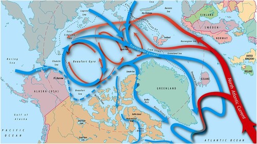
The motion of the ice and of the surface layer of the ocean in the Arctic regions are dominated by two prominent features: the Beaufort Gyre and the Transpolar Drift (TD) current; see (Serreze and Barry 2014, Timmermans and Marshall 2020) and figure 1. These two flows involve a wind-driven component, with wind blowing over the ice (which, in turn, affects the near-surface ocean below), coupled with a significant near-surface geostrophic flow. Our interest here is the TD and associated ice flow, the rôle of the geostrophic oceanic flow and the effects of the prevailing wind; outside the Canada basin, the mean surface winds in the Arctic Ocean blow nearly unidirectional from Russia towards Greenland. The near-surface geostrophic flow of the Transpolar Drift is driven by the sea-surface pressure gradients: the salinity differences between the relatively fresh water of the shallow Russian continental shelf (with a large amount of fresh water from river runoff), and the saltier ocean region adjacent to the North Atlantic waters, create a steric height-gradient of about 1 m across the Arctic Ocean (Charette et al. 2020). The flow in the Beaufort region is not involved in this process as its sea level, maintained by the circular gyre motion, is slightly higher than that of the Russian continental shelf (Jin et al. 2023). The TD transports ice and fresh surface-water from the East Siberian and Laptev Seas and, to a lesser extent, the Kara Sea (where new sea ice is constantly produced in the winter season, due to extremely low air temperatures – down to −40${}^{\circ }$C – and a strong offshore wind that drives the fresh ice out to the open sea) through the Fram Strait, although, under some conditions, there is a branch of the flow which curves towards the Beaufort Gyre and does not exit the Arctic Ocean. About 2000–3000 km${}^3$ of sea ice, per year, move along the TD, eventually reaching the North Atlantic, although we should note that there are significant variations over the year, and from year-to-year. Indeed, in extreme circumstances, the TD can reverse direction (Wilson et al. 2021). The position of the TD is determined by the Arctic Oscillation (AO), a large-scale weather pattern characterised by winds blowing from West to East close to 55${}^{\circ }$N. During the AO's positive phase (with lower-than-average air pressure over the Arctic, paired with higher-than-average pressure over the northern Pacific and Atlantic Oceans) these winds are reinforced and confine the colder air to the polar regions, while the TD shifts eastwards toward the Bering Strait, entraining additional Pacific water to that received from the Russian continental shelf. During a negative AO (with higher-than-average air pressure over the Arctic region and lower-than-average pressure over the northern Pacific and Atlantic Oceans), the strength of the winds in the belt is reduced, allowing southward penetrations of arctic airmasses and weakening the TD.

Figure 1. Schematic of the Arctic Ocean circulation (© Woods Hole Oceanographic Institution, J. Cook). Blue arrows indicate the surface circulation (the Beaufort Gyre and the Transpolar Drift current, with the main pathway of the Pacific Water dashed) and the pink-red arrows show the Atlantic Water circulation at intermediate depths – when the saltier Atlantic water reaches the Arctic, it sinks beneath the cool, fresh surface water. A halocline blocks the warmer Atlantic Water from direct contact with, and melting of, the overlying sea ice.

The TD, generally, moves faster than the deeper parts of the ocean, but slower than the surface ice. Buoy and satellite data (see Gascard and Metaxian 2008, Olason and Notz 2014, Ward and Tandon 2024) show that the TD travels, on average, at a speed of about $7.5\mathrm{cm}{\mathrm{s}}^{-1}$ within 5${}^{\circ }$ of the North Pole, but can reach speeds of $20\mathrm{cm}{\mathrm{s}}^{-1}$ as it flows through the Fram Strait, although our approach described here, based on the f-plane approximation around the North Pole, will not allow us to get close to the Fram Strait. The slower-moving ocean directly below the ice moves so that the Ekman component is in a direction to the right of the direction of the stress at the surface of the water; this stress is provided by the floating ice, but not necessarily aligned with the direction taken by the ice. The motion is controlled, jointly, by the prevailing wind conditions and the geostrophic flow near the surface; of course, as the wind field and the geostrophic flow change over time, so does the direction of the TD. In addition to these essentially global properties of the TD, detailed models that aim to describe the local dynamics and thermodynamics (and associated varying ice thickness) are readily constructed; an excellent overview can be found in Spall (2019). To this discussion of the dynamics, we might add chemical and mechanical investigations into the nature of the ice: its formation, structure and melting-processes (Leppäranta 2011, Wadhams 2014).

It is evident from the foregoing brief description of issues related to the near-surface flows in the Arctic Ocean, and the TD in particular, that this presents a complex system but, we will argue, there is a coherent and well-defined mathematical structure which underpins the dynamics – and that is our prime interest here. Further, we believe that the way forward in any careful study of such phenomena is to start from a firm and uncontested base: the general governing equations for a fluid, with suitable boundary and initial conditions. It is only in respect of the boundary conditions, in particular how to represent the air-ice-water interface, that modelling necessarily plays a rôle; without doubt, its choice is critical in helping us to understand the processes involved. Although we cannot expect to find a relevant exact solution to the full set of governing equations, we can be sure of the status of any approximate (asymptotic) procedure that we adopt. This does allow us to be precise about the errors, and to point the way to the construction of higher-order terms. The overall plan is eventually to add, progressively and systematically, more accurate details that are needed to provide as complete a picture as we would wish of the dynamics of this atmosphere-ice-ocean complex. The intention in this paper is therefore simply to lay the foundations, both as – we hope – a useful additional tool for the oceanographers and, perhaps, also to excite the interest of mathematicians who are unfamiliar with these types of problem. And, as it happens, the TD presents some intriguing challenges; how to characterise these, and deal with them, is our first task, and paramount is a significant technical issue.

The conventional formulation involves the introduction of a set of rotating, spherical coordinates, using the familiar azimuthal and meridional angles (often referred to as geographical coordinates). However, the resulting equations of motion are inadmissible at the poles because singularities necessarily exist there: the associated tangent unit vectors are not well-defined at these two points on the sphere; see (Constantin and Johnson 2024) for a presentation of the issues. Some investigations of arctic ocean flow that rely on geographical coordinates avoid regions near the North Pole (see Vallis 2005, Talley et al. 2011, Constantin 2022a,b). On the other hand, intricate manoeuvres have been invented in order to extract something relevant by using geographical coordinates close to the North Pole (LeBlond 1964, Thomas and Lux 1978, Yang 1987, Nof 1990), but these are far from satisfactory since the singularity issue is not resolved: these approximations cannot be derived systematically from the geographical coordinates since the coefficients of the Taylor expansion become divergent at the North Pole. This difficulty is due to the particular choice of spherical coordinates, the problem being remedied by rotating the geographical coordinates so that the unavoidable singularities now appear at two (diametrically opposite) points on the Equator. Such a reformulation then allows a mathematically satisfactory description of ocean flows near and at the poles. We should comment that, although the idea is simple, the required transformations are rather involved; the details are carefully developed in Constantin and Johnson (2023) where near-surface currents in the Arctic Ocean are discussed, with only the thin-shell approximation being invoked. Here, we use a reduced version of these equations, further simplified on the basis of the f-plane approximation, but with an appropriate model for the surface boundary condition (extending the earlier work), one which, we believe, adequately describes the interaction between the air, the ice and the surface of the ocean. (The use of this more sophisticated and accurate boundary condition, without recourse to any approximations of the f-plane-type, will be examined in a forthcoming paper.) The flow in the near-surface necessarily involves an Ekman-type balance – the simple and expected structure – but superimposed on a suitable geostrophic oceanic flow, which is the dominant contributor to the motion. Further, we also include the possibility that the ice cover can be moving at different velocities at different positions, and might evolve (e.g. change thickness along its path), but always within the steady-state scenario.

The plan for this paper is the following. In section 2 we present the governing equations (taken from Constantin and Johnson 2023, but with the f-plane approximation invoked); then in section 3 we provide a formulation of the boundary condition at the surface which describes the presence of ice, and the interaction between wind, ice and water. In section 4, a solution is presented which describes the wind driving the ice over the Transpolar Drift current, and in section 5 we summarise and comment on this solution.

2. Governing equations

In this analysis, we take the Earth to be sphere (of radius 6371 km) and so ignore the effects of the shape of the Earth's geoid. As demonstrated in Constantin and Johnson (2021), this correction is readily included, but here it is inconsequential to the analysis of the TD (see the discussion in White 2002), so we choose to set it aside. 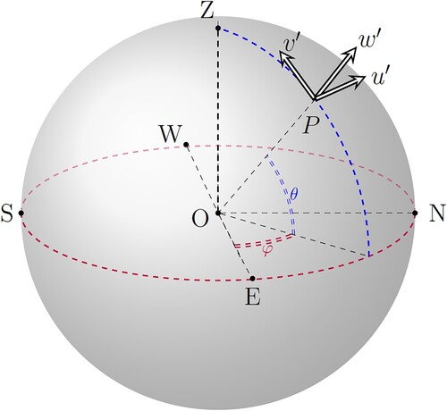We consider a set of (right-handed) spherical coordinates $(\phi ,\theta ,r^{\prime })$: $r^{\prime }$ is the distance (radius) from the centre of the sphere, $\theta \in [-\frac{\pi }{2},\frac{\pi }{2}]$ is a meridional angle and $\phi \in [0,2\pi )$ is an azimuthal angle. We choose the underlying fixed coordinate axes, relative to the centre of the Earth, to be pointing towards the North Pole (N), the Null Island (Z), which sits in international waters in the Gulf of Guinea (where the prime meridian and the equator intersect), and to the East (E); see figure 2. Associated with the unit vectors in this $(\phi ,\theta ,r^{\prime })$-system we have the velocity components $(u^{\prime },v^{\prime },w^{\prime })\equiv {\mathbf{u}}^{\prime }$, so that $u^{\prime }$ points from East to West, and $v^{\prime }$ from North to South. (We use primes, throughout the formulation of the problem, to denote physical (dimensional) variables; these will be removed when we non-dimensionalise.) The $(\phi ,\theta ,r^{\prime })$-system defines points on the stationary sphere, described by rotating the geographical coordinate system; in this new system, the two points where the tangent unit vectors are not well-defined are Z and its antipode (both located on the Equator). The transformation to this new system, from the geographical one, is described in detail in Constantin and Johnson (2023).

Figure 2. Coordinates and velocity components associated with the rotated system.

The governing equations for ocean flow, derived in Constantin and Johnson (2023) in this rotated coordinate system, are the Navier-Stokes equation (1) $\begin{array}{rl}& {\rho }^{\prime }\frac{\mathrm{D}}{\mathrm{D}{t}^{\prime }}(u^{\prime },v^{\prime },w^{\prime })+\frac{{\rho }^{\prime }}{r^{\prime }}(-u^{\prime }{v}^{\prime }\tan \theta +u^{\prime }{w}^{\prime },{u^{\prime }}^2\tan \theta +v^{\prime }{w}^{\prime },-{u^{\prime }}^2-{v^{\prime }}^2)\\ & +2{\Omega }^{\prime }(-\sin \mathrm{\phi cos}\theta v^{\prime }-\sin \mathrm{\phi sin}\theta w^{\prime },\sin \mathrm{\phi cos}\theta u^{\prime }-\cos \phi w^{\prime },\sin \mathrm{\phi sin}\theta u^{\prime }+\cos \phi v^{\prime })\\ & +r^{\prime }{\Omega }^{\prime 2}(\sin \mathrm{\phi cos}\mathrm{\phi cos}\theta ,{\sin }^2\mathrm{\phi sin}\mathrm{\theta cos}\theta ,-{\sin }^2\phi {\sin }^2\theta -{\cos }^2\phi )\\ & =-{\mathrm{\nabla }}^{\prime }{p}^{\prime }+{\rho }^{\prime }(0,0,-g^{\prime }\frac{R^{\prime 2}}{r^{\prime 2}})+{\mathrm{\nabla }}_{\mu }^{\prime 2}(u^{\prime },v^{\prime },w^{\prime })\\ & -\frac{1}{r^{\prime 2}{\cos }^2\theta }({\mu }_h^{\prime }{u}^{\prime },{\mu }_h^{\prime }{v}^{\prime },2{\mu }_{\nu }^{\prime }(w^{\prime }{\cos }^2\theta -v^{\prime }\sin \theta \cos \theta ))+\frac{2{\mu }_h^{\prime }}{r^{\prime 2}}\frac{\mathrm{\partial }}{\mathrm{\partial }\theta }(0,w^{\prime },-v^{\prime })\\ & +\frac{2{\mu }_h^{\prime }}{r^{\prime 2}\cos \theta }\frac{\mathrm{\partial }}{\mathrm{\partial }\phi }(w^{\prime }-v^{\prime }\tan \theta ,u^{\prime }\tan \theta ,-u^{\prime })+\frac{\mathrm{d}{\mu }_{\nu }^{\prime }}{\mathrm{d}{r}^{\prime }}{r}^{\prime }\frac{\mathrm{\partial }}{\mathrm{\partial }{r}^{\prime }}(\frac{u^{\prime }}{r^{\prime }},\frac{v^{\prime }}{r^{\prime }},\frac{w^{\prime }}{r^{\prime }})\\ & +(\frac{1}{r^{\prime }\cos \theta }\frac{\mathrm{d}{\mu }_h^{\prime }}{\mathrm{d}{r}^{\prime }}\frac{\mathrm{\partial }}{\mathrm{\partial }\phi },\frac{1}{r^{\prime }}\frac{\mathrm{d}{\mu }_h^{\prime }}{\mathrm{d}{r}^{\prime }}\frac{\mathrm{\partial }}{\mathrm{\partial }\theta },\frac{\mathrm{d}{\mu }_{\nu }^{\prime }}{\mathrm{d}{r}^{\prime }}\frac{\mathrm{\partial }}{\mathrm{\partial }{r}^{\prime }})(r^{\prime }{w}^{\prime }),\end{array}$(1) and the equation of mass conservation (2) $\frac{1}{r^{\prime }\cos \theta }\frac{\mathrm{\partial }{u}^{\prime }}{\mathrm{\partial }\phi }+\frac{1}{r^{\prime }\cos \theta }\frac{\mathrm{\partial }}{\mathrm{\partial }\theta }(v^{\prime }\cos \theta )+\frac{1}{r^{\prime 2}}\frac{\mathrm{\partial }}{\mathrm{\partial }{r}^{\prime }}(r^{\prime 2}{w}^{\prime })=0,$(2) where $t^{\prime }$ is time, $g^{\prime }\approx 9.81\mathrm{m}{\mathrm{s}}^{-2}$ is the average acceleration of gravity at the surface of the Earth of radius $R^{\prime }\approx 6371\mathrm{km}$, ${\Omega }^{\prime }\approx 7.29\times {10}^{-5}\mathrm{rad}{\mathrm{s}}^{-1}$ is the constant rate of rotation of the Earth around the polar axis, $p^{\prime }(\phi ,\theta ,r^{\prime },t^{\prime })$ is the pressure in the water, ${\rho }^{\prime }$ is the water's density (taken to be constant, which is appropriate for the upper layer of the Arctic Ocean where the TD resides), ${\mu }_{\nu }^{\prime }$ and ${\mu }_h^{\prime }$ are the coefficients of the vertical and horizontal dynamic eddy viscosities, respectively (each being a function of only $r^{\prime }$), and (3) $\begin{array}{rl}& \frac{\mathrm{D}}{\mathrm{D}{t}^{\prime }}\equiv (\frac{\mathrm{\partial }}{\mathrm{\partial }{t}^{\prime }}+\frac{u^{\prime }}{r^{\prime }\cos \theta }\frac{\mathrm{\partial }}{\mathrm{\partial }\phi }+\frac{v^{\prime }}{r^{\prime }}\frac{\mathrm{\partial }}{\mathrm{\partial }\theta }+w^{\prime }\frac{\mathrm{\partial }}{\mathrm{\partial }{r}^{\prime }});{\mathrm{\nabla }}^{\prime }\equiv (\frac{1}{r^{\prime }\cos \theta }\frac{\mathrm{\partial }}{\mathrm{\partial }\phi },\frac{1}{r^{\prime }}\frac{\mathrm{\partial }}{\mathrm{\partial }\theta },\frac{\mathrm{\partial }}{\mathrm{\partial }{r}^{\prime }});\end{array}$(3) (4) $\begin{array}{rl}& {\mathrm{\nabla }}_{\mu }^{\prime 2}\equiv {\mu }_{\nu }^{\prime }(\frac{{\mathrm{\partial }}^2}{\mathrm{\partial }{r}^{\prime 2}}+\frac{2}{r^{\prime }}\frac{\mathrm{\partial }}{\mathrm{\partial }{r}^{\prime }})+\frac{{\mu }_h^{\prime }}{r^{\prime 2}}(\frac{1}{{\cos }^2\theta }\frac{{\mathrm{\partial }}^2}{\mathrm{\partial }{\phi }^2}+\frac{{\mathrm{\partial }}^2}{\mathrm{\partial }{\theta }^2}-\tan \theta \frac{\mathrm{\partial }}{\mathrm{\partial }\theta }).\end{array}$(4) Taking the two dynamic eddy viscosities to be equal and constant (${\mu }_{\nu }^{\prime }={\mu }_h^{\prime }={\mu }^{\prime }$), it is convenient to redefine the pressure as (5) $p^{\prime }=\frac{{\rho }^{\prime }{g}^{\prime }{R}^{\prime 2}}{r^{\prime }}+\frac{1}{2}{\rho }^{\prime }{r}^{\prime 2}{\Omega }^{\prime 2}({\sin }^2\phi {\sin }^2\theta +{\cos }^2\phi )+P^{\prime }(\phi ,\theta ,r^{\prime },t^{\prime }),$(5) and then nondimensionalise according to (6) $z^{\prime }=D^{\prime }z,(u^{\prime },v^{\prime },w^{\prime })=U^{\prime }(u,v,\kappa w),P^{\prime }={\rho }^{\prime }{U}^{\prime 2}P,t^{\prime }=\frac{R^{\prime }}{U^{\prime }}t,$(6) where $r^{\prime }=R^{\prime }+z^{\prime }$, $D^{\prime }$ is a suitable depth scale, $U^{\prime }$ is a suitable average speed scale and κ is a constant to be chosen. In the thin-shell approximation, i.e. in the limit $\epsilon =\frac{D^{\prime }}{R^{\prime }}\to 0,$ which requires the choice $\kappa =\epsilon$ for consistency, the governing equations, retaining the dominant terms, can be written in the rotated coordinates (see Constantin and Johnson 2023) as (7) $\begin{array}{rl}& (\frac{\mathrm{\partial }}{\mathrm{\partial }t}+\frac{u}{\cos \theta }\frac{\mathrm{\partial }}{\mathrm{\partial }\phi }+v\frac{\mathrm{\partial }}{\mathrm{\partial }\theta }+w\frac{\mathrm{\partial }}{\mathrm{\partial }z})(u,v,0)+(-\mathrm{uvtan}\theta ,u^2\tan \theta ,-u^2-v^2)\\ & +2\omega (-v\sin \mathrm{\phi cos}\theta v,u\sin \mathrm{\phi cos}\theta ,u\sin \mathrm{\phi sin}\theta +v\cos \phi )\\ & =-(\frac{1}{\cos \theta }\frac{\mathrm{\partial }P}{\mathrm{\partial }\phi },\frac{\mathrm{\partial }P}{\mathrm{\partial }\theta },\frac{1}{\epsilon }\frac{\mathrm{\partial }P}{\mathrm{\partial }z})+\frac{1}{R_e}\frac{{\mathrm{\partial }}^2}{\mathrm{\partial }{z}^2}(u,v,0),\end{array}$(7) and (8) $\frac{\mathrm{\partial }u}{\mathrm{\partial }\phi }+\frac{\mathrm{\partial }}{\mathrm{\partial }\theta }(\mathrm{ucos}\theta )+\cos \theta \frac{\mathrm{\partial }w}{\mathrm{\partial }z}=0.$(8) where (9) $\omega =\frac{{\Omega }^{\prime }{R}^{\prime }}{U^{\prime }},R_e=\frac{{\rho }^{\prime }{U}^{\prime }{D}^{\prime 2}}{{\mu }^{\prime }{R}^{\prime }}.$(9) Now the formulation that we wish to develop here focusses on the surface layer of the ocean, for which the appropriate depth scale (measuring the Ekman-layer thickness) is (10) $D^{\prime }=\sqrt{\frac{{\mu }^{\prime }}{{\rho }^{\prime }{\Omega }^{\prime }}}$(10) (about 20 m since ${\mu }^{\prime }/{\rho }^{\prime }\approx 0.025{\mathrm{m}}^2{\mathrm{s}}^{-1}$ is adequate for near-surface arctic ocean – see Morison and McPhee 2001) and then (11) $\frac{1}{R_e}=\frac{R^{\prime }{\Omega }^{\prime }}{U^{\prime }}=\omega .$(11) The natural choice (leading to a consistent asymptotic representation – see Constantin and Johnson 2019, Johnson 2022, 2023) is to set (12) $\omega =\frac{\overline{\omega }}{\epsilon }\mathrm{with}\overline{\omega }=\frac{D^{\prime }{\Omega }^{\prime }}{U^{\prime }}=\mathrm{O}(1)\mathrm{as}\epsilon \to 0.$(12) We couple this with the use of the f-plane approximation, and associated tangent-plane coordinates $x=\phi \cos \theta ,y=\theta ,$ taking the origin at the North Pole where $\phi =\frac{\pi }{2}$, $\theta =0$. Thus x points from East to West through the North Pole, and y points from the North Pole southwards directly towards the Fram Strait and Null Island. The equations for steady flow then reduce to a very familiar form (but only because we have rotated the more usual choice of spherical coordinates). Retaining the dominant terms required for our solution, we obtain (13) $\begin{array}{rl}-2\frac{\overline{\omega }}{\epsilon }v& =\frac{\overline{\omega }}{\epsilon }\frac{{\mathrm{\partial }}^{2}u}{\mathrm{\partial }{z}^2}-\frac{\mathrm{\partial }P}{\mathrm{\partial }x},\end{array}$(13) (14) $\begin{array}{rl}2\frac{\overline{\omega }}{\epsilon }u& =\frac{\overline{\omega }}{\epsilon }\frac{{\mathrm{\partial }}^{2}v}{\mathrm{\partial }{z}^2}-\frac{\mathrm{\partial }P}{\mathrm{\partial }y},\end{array}$(14) (15) $\begin{array}{rl}-(u^2+v^2)& =-\frac{1}{\epsilon }\frac{\mathrm{\partial }P}{\mathrm{\partial }z},\end{array}$(15) (16) $\begin{array}{rl}\frac{\mathrm{\partial }u}{\mathrm{\partial }x}+\frac{\mathrm{\partial }v}{\mathrm{\partial }y}+\frac{\mathrm{\partial }w}{\mathrm{\partial }z}& =0.\end{array}$(16) The vertical component of vorticity is then (17) $\Gamma =\frac{\mathrm{\partial }v}{\mathrm{\partial }x}-\frac{\mathrm{\partial }u}{\mathrm{\partial }y}.$(17) To accommodate, in the near-surface layer of the ocean, a background geostrophic flow ${\mathbf{u}}_g=(u_g,v_g)$ which does not vary with depth we write (18) $P=\frac{1}{\epsilon }{P}_g+\hat{p}.$(18) We can now define the geostrophic flow as (19) $(u_g,v_g)=\frac{1}{2\overline{\omega }}(-\frac{\mathrm{\partial }{P}_g}{\mathrm{\partial }y},\frac{\mathrm{\partial }{P}_g}{\mathrm{\partial }x})$(19) with (20) $\frac{\mathrm{\partial }{P}_g}{\mathrm{\partial }z}=0,$(20) and the compatibiltiy condition (21) $\frac{\mathrm{\partial }{u}_g}{\mathrm{\partial }x}+\frac{\mathrm{\partial }{v}_g}{\mathrm{\partial }y}=0,$(21) required to ensure that $\frac{{\mathrm{\partial }}^2{P}_g}{\mathrm{\partial }x\mathrm{\partial y}}$ is well-defined. Note that we could allow the geostrophic flow to have a viscous contribution (and so a depth-variation), but this is usually ignored in the classical description; in keeping with this, we do not explore that option here.

Finally, we set $\mathbf{u}={\mathbf{u}}_g+{\mathbf{u}}_E$ and so obtain (22) $\begin{array}{rl}-2v_E& =\frac{{\mathrm{\partial }}^2{u}_E}{\mathrm{\partial }{z}^2},\end{array}$(22) (23) $\begin{array}{rl}2u_E& =\frac{{\mathrm{\partial }}^2{v}_E}{\mathrm{\partial }{z}^2},\end{array}$(23) (24) $\begin{array}{rl}\frac{\mathrm{\partial }\hat{p}}{\mathrm{\partial }z}& =0,\end{array}$(24) (25) $\begin{array}{rl}\frac{\mathrm{\partial }{u}_E}{\mathrm{\partial }x}+\frac{\mathrm{\partial }{v}_E}{\mathrm{\partial }y}+\frac{\mathrm{\partial }{w}_E}{\mathrm{\partial }z}& =0,\end{array}$(25) at leading order as $\epsilon \to 0$, which defines the Ekman component of the flow and any upwelling/downwelling generated by it (and described by $w_E$); the vorticity is $\Gamma ={\Gamma }_g+{\Gamma }_E$ with (26) ${\Gamma }_g=\frac{\mathrm{\partial }{v}_g}{\mathrm{\partial }x}-\frac{\mathrm{\partial }{u}_g}{\mathrm{\partial }y},{\Gamma }_E=\frac{\mathrm{\partial }{v}_E}{\mathrm{\partial }x}-\frac{\mathrm{\partial }{u}_E}{\mathrm{\partial }y}.$(26) In this formulation, we note that the two components that contribute to the flow of the ocean – the geostrophic and Ekman flows – are the same order in ε, although we expect the former to be rather larger than the latter.

3. Surface boundary condition

The fundamental model that we use, and which underpins the stress conditions at the air-ice-water interface, is a frictional drag proportional to the square of the relative speeds of the two components that slide over one another. The drag of the ice over the water provides a shear at the surface of the ocean; this then gives the condition (27) ${\mu }^{\prime }\frac{\mathrm{\partial }{\mathbf{u}}^{\prime }}{\mathrm{\partial }z}=-{\rho }^{\prime }{C}_{\mathrm{oi}}|{\mathbf{u}}^{\prime }-{\mathbf{u}}_i^{\prime }|({\mathbf{u}}^{\prime }-{\mathbf{u}}_i^{\prime }),$(27) where ${\rho }^{\prime }$ is the density of the surface water (which we take to be constant throughout the surface layer), $C_{\mathrm{oi}}\approx 5.5\times {10}^{-3}$ is the nondimensional drag coefficient of ice on water and ${\mathbf{u}}_i^{\prime }$ is the velocity of the ice. For the ice, the difference in stress, above and below, generates an internal stress (Hibler 1979, Spall 2019). The general structure of this stress is quite involved, but here we choose to follow (Spall 2019), where it is argued that the most important effect of this stress difference is simply to produce an internal ice pressure. This, in turn, is modelled by Hibler (1979) and Spall (2019) as proportional to the thickness of the ice, so we write (28) ${\rho }_a^{\prime }{C}_{\mathrm{ai}}|{\mathbf{u}}_a^{\prime }-{\mathbf{u}}_i^{\prime }|({\mathbf{u}}_a^{\prime }-{\mathbf{u}}_i^{\prime })+{\rho }^{\prime }{C}_{\mathrm{oi}}|{\mathbf{u}}^{\prime }-{\mathbf{u}}_i^{\prime }|({\mathbf{u}}^{\prime }-{\mathbf{u}}_i^{\prime })+{\mathrm{\nabla }}^{\prime }(-{\mathrm{\Pi }}^{\prime }{h}^{\prime })=\mathbf{0},$(28) where ${\rho }_a^{\prime }$ is the density of the air just above the surface of the ice, $C_{\mathrm{ai}}\approx 1.8\times {10}^{-3}$ is the drag coefficient of air-over-ice, the vector ${\mathbf{u}}_a^{\prime }$ is the velocity of the wind near the surface, ${\mathrm{\Pi }}^{\prime }$ is a positive constant which is proportional to the ice strength, $h^{\prime }(x^{\prime },y^{\prime })$ is the thickness of the ice and ${\mathrm{\nabla }}^{\prime }=(\frac{\mathrm{\partial }}{\mathrm{\partial }{x}^{\prime }},\frac{\mathrm{\partial }}{\mathrm{\partial }{y}^{\prime }});$ all the above are written in dimensional variables. A contribution from the variation in ambient sea-surface height is ignored, and it is certainly not critical to the mechanism described here; Spall 2019 argues that this is a smaller-order correction (but this could readily be included in a more careful treatment). In addition, we require an equation which describes how the thickness of the ice evolves; this is a continuity equation which balances horizontal-flux divergence with the formation/loss due to cooling/heating at the surface of the ice. The heat loss is proportional to the temperature change across the ice (freezing temperature of the ice minus the surface temperature of the ice), which we take to be constant, and inversely proportional to the thickness of the ice (see Spall 2019); thus we have (29) ${\mathrm{\nabla }}^{\prime }\cdot ({\mathbf{u}}_i^{\prime }{h}^{\prime })=\frac{{\Gamma }^{\prime }}{h^{\prime }},$(29) where ${\Gamma }^{\prime }$ is a positive constant. We note immediately that this model cannot permit the ice to reach zero thickness (although there are solutions for which the thickness decreases and can approach zero); in any event, this is not a significant issue here because the f-plane approximation cannot reasonably be applied simultaneously across the North Pole and then as far as the Fram Strait. Altimetric and in situ measurements (see Kwok 2018) show that within 5${}^{\circ }$ of the North Pole the mean ice-thickness is about 2–4 m. While we cannot allow $h^{\prime }=0$ in equation (29(29) ${\mathrm{\nabla }}^{\prime }\cdot ({\mathbf{u}}_i^{\prime }{h}^{\prime })=\frac{{\Gamma }^{\prime }}{h^{\prime }},$(29) ), our results are valid even if the ice thickness is considerably reduced to, say, 10$\mathrm{\%}$ of the initial value. However, a description of the dynamics through the Fram Strait (where the ice thickness becomes essentially zero), and beyond, requires a new model.

The two drag conditions, (27(27) ${\mu }^{\prime }\frac{\mathrm{\partial }{\mathbf{u}}^{\prime }}{\mathrm{\partial }z}=-{\rho }^{\prime }{C}_{\mathrm{oi}}|{\mathbf{u}}^{\prime }-{\mathbf{u}}_i^{\prime }|({\mathbf{u}}^{\prime }-{\mathbf{u}}_i^{\prime }),$(27) ) and (28(28) ${\rho }_a^{\prime }{C}_{\mathrm{ai}}|{\mathbf{u}}_a^{\prime }-{\mathbf{u}}_i^{\prime }|({\mathbf{u}}_a^{\prime }-{\mathbf{u}}_i^{\prime })+{\rho }^{\prime }{C}_{\mathrm{oi}}|{\mathbf{u}}^{\prime }-{\mathbf{u}}_i^{\prime }|({\mathbf{u}}^{\prime }-{\mathbf{u}}_i^{\prime })+{\mathrm{\nabla }}^{\prime }(-{\mathrm{\Pi }}^{\prime }{h}^{\prime })=\mathbf{0},$(28) ), are to be evaluated at the surface, which we take to be z = 0 for both the upper and lower surfaces of the ice; this is reasonable, even in the light of the thin-shell approximation, because the thickness of the ice is much smaller than the scale depth that we have used here. Thus, with the non-dimensionalisation that we have already introduced, we obtain the boundary conditions in the form (30) $\begin{array}{rl}& \frac{\mathrm{\partial }\mathbf{u}}{\mathrm{\partial }z}=-c_{\mathrm{oi}}|\mathbf{u}-{\mathbf{u}}_i|(\mathbf{u}-{\mathbf{u}}_i)=r_a{c}_{\mathrm{ai}}|{\mathbf{u}}_a-{\mathbf{u}}_i|({\mathbf{u}}_a-{\mathbf{u}}_i)-\alpha (\frac{\mathrm{\partial }h}{\mathrm{\partial }x},\frac{\mathrm{\partial }h}{\mathrm{\partial }y})\mathrm{on}z=0,\\ & (\frac{\mathrm{\partial }}{\mathrm{\partial }x},\frac{\mathrm{\partial }}{\mathrm{\partial }y})\cdot ({\mathbf{u}}_{i}h)=\frac{\Gamma }{h},\end{array}$(30) where (31) $\begin{array}{r}{c}_{\mathrm{oi}}=C_{\mathrm{oi}}\frac{{\rho }^{\prime }{U}^{\prime }{D}^{\prime }}{{\mu }^{\prime }},c_{\mathrm{oi}}=C_{\mathrm{ai}}\frac{{\rho }^{\prime }{U}^{\prime }{D}^{\prime }}{{\mu }^{\prime }},r_a=\frac{{\rho }_a^{\prime }}{{\rho }^{\prime }},\alpha =\frac{{\mathrm{\Pi }}^{\prime }{H}^{\prime }{D}^{\prime }}{R^{\prime }{U}^{\prime }{\mu }^{\prime }},\Gamma =\frac{{\Gamma }^{\prime }{R}^{\prime }}{U^{\prime }{H}^{\prime 2}},\end{array}$(31) with $h^{\prime }=H^{\prime }h$, where $H^{\prime }$ is an average or typical thickness of the ice. All the nondimensional parameters that we have introduced here are treated as fixed, i.e. $\mathrm{O}(1)$, relative to the underlying limiting process which is predicated on the thin-shell approximation.

4. The wind-ice-ocean solution

We now develop a solution of equations (22(22) $\begin{array}{rl}-2v_E& =\frac{{\mathrm{\partial }}^2{u}_E}{\mathrm{\partial }{z}^2},\end{array}$(22) )–(25(25) $\begin{array}{rl}\frac{\mathrm{\partial }{u}_E}{\mathrm{\partial }x}+\frac{\mathrm{\partial }{v}_E}{\mathrm{\partial }y}+\frac{\mathrm{\partial }{w}_E}{\mathrm{\partial }z}& =0,\end{array}$(25) ), which satisfies the boundary conditions (30(30) $\begin{array}{rl}& \frac{\mathrm{\partial }\mathbf{u}}{\mathrm{\partial }z}=-c_{\mathrm{oi}}|\mathbf{u}-{\mathbf{u}}_i|(\mathbf{u}-{\mathbf{u}}_i)=r_a{c}_{\mathrm{ai}}|{\mathbf{u}}_a-{\mathbf{u}}_i|({\mathbf{u}}_a-{\mathbf{u}}_i)-\alpha (\frac{\mathrm{\partial }h}{\mathrm{\partial }x},\frac{\mathrm{\partial }h}{\mathrm{\partial }y})\mathrm{on}z=0,\\ & (\frac{\mathrm{\partial }}{\mathrm{\partial }x},\frac{\mathrm{\partial }}{\mathrm{\partial }y})\cdot ({\mathbf{u}}_{i}h)=\frac{\Gamma }{h},\end{array}$(30) ), and which also provides a description of how the thickness of the ice changes, in accordance with (31(31) $\begin{array}{r}{c}_{\mathrm{oi}}=C_{\mathrm{oi}}\frac{{\rho }^{\prime }{U}^{\prime }{D}^{\prime }}{{\mu }^{\prime }},c_{\mathrm{oi}}=C_{\mathrm{ai}}\frac{{\rho }^{\prime }{U}^{\prime }{D}^{\prime }}{{\mu }^{\prime }},r_a=\frac{{\rho }_a^{\prime }}{{\rho }^{\prime }},\alpha =\frac{{\mathrm{\Pi }}^{\prime }{H}^{\prime }{D}^{\prime }}{R^{\prime }{U}^{\prime }{\mu }^{\prime }},\Gamma =\frac{{\Gamma }^{\prime }{R}^{\prime }}{U^{\prime }{H}^{\prime 2}},\end{array}$(31) ). Although the physical problem is more naturally presented as a prescribed wind blowing over an ice sheet under which the ocean moves (with a component provided by some known geostrophic flow), the mathematical problem is best approached slightly differently. The starting point, in this case, is to find the relevant (Ekman) solution of equations (22(22) $\begin{array}{rl}-2v_E& =\frac{{\mathrm{\partial }}^2{u}_E}{\mathrm{\partial }{z}^2},\end{array}$(22) )–(25(25) $\begin{array}{rl}\frac{\mathrm{\partial }{u}_E}{\mathrm{\partial }x}+\frac{\mathrm{\partial }{v}_E}{\mathrm{\partial }y}+\frac{\mathrm{\partial }{w}_E}{\mathrm{\partial }z}& =0,\end{array}$(25) ), and then impose the boundary conditions, given the geostrophic flow in the surface layer of the ocean. This enables both the motion of the ice, and the wind blowing over it, to be determined. Having obtained this solution, which clearly is unique for given Ekman and geostrophic flows, it can then be interpreted in reverse: the wind blowing over the ice which, in turn, contributes to the motion of the ocean. Throughout, the guiding principle is to recover something close to the observed motions of the wind, ice and ocean. The aim is then to show that what is observed is consistent with the governing equations and boundary conditions (i.e. appropriate solutions do exist) and, perhaps more significantly, how this comes about.

We start with a model for the underlying geostrophic near-surface ocean flow, which we write in terms of a stream function $\psi =-\frac{b}{2m}(y+\mathrm{mx}{)}^2+u_{0}y-v_{0}x$ so that (32) $\begin{array}{rl}{u}_g& =\frac{\mathrm{\partial }\psi }{\mathrm{\partial }y}=u_0-\frac{b}{m}(y+\mathrm{mx}),\end{array}$(32) (33) $\begin{array}{rl}{v}_g& =-\frac{\mathrm{\partial }\psi }{\mathrm{\partial }x}=v_0+b(y+\mathrm{mx}),\end{array}$(33) where $u_0$, $v_0$, b and m are positive constants. We choose these constants so that, in a neighbourhood of the North Pole, both $u_g$ and $v_g$ are positive, with the flow predominantly in the y-direction (which mimics the flow across the North Pole towards the Fram Strait). A solution of equations (22(22) $\begin{array}{rl}-2v_E& =\frac{{\mathrm{\partial }}^2{u}_E}{\mathrm{\partial }{z}^2},\end{array}$(22) )–(25(25) $\begin{array}{rl}\frac{\mathrm{\partial }{u}_E}{\mathrm{\partial }x}+\frac{\mathrm{\partial }{v}_E}{\mathrm{\partial }y}+\frac{\mathrm{\partial }{w}_E}{\mathrm{\partial }z}& =0,\end{array}$(25) ) is the classical Ekman flow (decaying with depth) associated with the surface stress generated by the ice; this is (34) $\begin{array}{rl}{u}_E& =a(x,y){\mathrm{e}}^z\cos (z-\mathrm{k\pi }),\end{array}$(34) (35) $\begin{array}{rl}{v}_E& =a(x,y){\mathrm{e}}^z\sin (z-\mathrm{k\pi }),\end{array}$(35) where k is a constant chosen for simplicity here – the flow is in a fixed direction at the surface – but this could be relaxed (with $k=k(x,y)$). For k>0 and with the stress in the direction $\frac{\pi }{4}-\mathrm{k\pi }$, we shall find that we have made a choice which corresponds to the observed motions of the TD across the North Pole and which, we note, also permits a variable speed (by virtue of $a(x,y)$). This Ekman flow is evaluated at the surface, z = 0, and then combined with the geostrophic flow to give the Transpolar Drift current (TDc) at the surface of the ocean: (36) $\begin{array}{rl}u& =u_0-\frac{b}{m}(y+\mathrm{mx})+a(x,y)\cos (-\mathrm{k\pi }),\end{array}$(36) (37) $\begin{array}{rl}v& =v_0+b(y+\mathrm{mx})+a(x,y)\sin (-\mathrm{k\pi }).\end{array}$(37) We note that, for constant speeds, i.e. constant geostrophic flow and constant Ekman flow at the surface, which requires b = 0 and $a=\mathrm{constant}$, the Transpolar Drift current is then also a constant vector. Since the geostrophic vorticity of the flow (36(36) $\begin{array}{rl}u& =u_0-\frac{b}{m}(y+\mathrm{mx})+a(x,y)\cos (-\mathrm{k\pi }),\end{array}$(36) )–(37(37) $\begin{array}{rl}v& =v_0+b(y+\mathrm{mx})+a(x,y)\sin (-\mathrm{k\pi }).\end{array}$(37) ) is constant, ${\Gamma }_g=b+\frac{b}{m},$ suitable variations of $a(x,y)$ can accommodate the possibility of a sign change of the vorticity $\Gamma ={\Gamma }_g+{\Gamma }_E$ of the Transpolar Drift current at the surface, given that ${\Gamma }_E=\frac{\mathrm{\partial }a}{\mathrm{\partial }x}\cos (-\mathrm{k\pi })-\frac{\mathrm{\partial }a}{\mathrm{\partial }y}\sin (-\mathrm{k\pi })\mathrm{on}z=0.$ This captures an often observed feature of the Transpolar Drift current, connecting regions near the typically anticyclonic (negative) vorticity of the Beaufort gyre to eastern regions of the Arctic Ocean, of mostly cyclonic (positive) vorticity – see (Morison et al. 2021). The orientation of the Transpolar Drift current near the North Pole provides a strong indication of whether the Arctic Ocean circulation is dominated by the anticyclonic (clockwise) state of a large Beaufort Gyre, or by the cyclonic (counterclockwise) state of its Eurasian side (Morison et al. 2018). The steady geostrophic flow with velocity (32(32) $\begin{array}{rl}{u}_g& =\frac{\mathrm{\partial }\psi }{\mathrm{\partial }y}=u_0-\frac{b}{m}(y+\mathrm{mx}),\end{array}$(32) )–(33(33) $\begin{array}{rl}{v}_g& =-\frac{\mathrm{\partial }\psi }{\mathrm{\partial }x}=v_0+b(y+\mathrm{mx}),\end{array}$(33) ) occurs along streamlines. For a unidirectional geostrophic flow near the North Pole we set b = 0, and an orientation towards the Fram Strait requires $u_0=0$ and $v_0>0$. This direction is enforced if $u_E=0$ at the surface z = 0, corresponding to the choice $k=\frac{1}{2}$ for the Ekman flow, with the linear function $a(x,y)=a_0+a_{1}y$ with $a_0<0$ and $a_1<0$ accommodating an acceleration towards the Fram Strait. The vertical velocity can now be found from (25(25) $\begin{array}{rl}\frac{\mathrm{\partial }{u}_E}{\mathrm{\partial }x}+\frac{\mathrm{\partial }{v}_E}{\mathrm{\partial }y}+\frac{\mathrm{\partial }{w}_E}{\mathrm{\partial }z}& =0,\end{array}$(25) ), coupled with the boundary condition w = 0 on z = 0: $w_E=\frac{a_1}{2}\{\sqrt{2}{\mathrm{e}}^z\sin (z+\frac{\pi }{4})-1\},-1\le z\le 0.$ Since $a_1<0$ we conclude that, in this scenario, we expect upwelling along the path of the Transpolar Drift from the North Pole towards the Fram Strait – this being the trend for the period 1979–2014 (Ma et al. 2017).

The first equation in the boundary condition (30(30) $\begin{array}{rl}& \frac{\mathrm{\partial }\mathbf{u}}{\mathrm{\partial }z}=-c_{\mathrm{oi}}|\mathbf{u}-{\mathbf{u}}_i|(\mathbf{u}-{\mathbf{u}}_i)=r_a{c}_{\mathrm{ai}}|{\mathbf{u}}_a-{\mathbf{u}}_i|({\mathbf{u}}_a-{\mathbf{u}}_i)-\alpha (\frac{\mathrm{\partial }h}{\mathrm{\partial }x},\frac{\mathrm{\partial }h}{\mathrm{\partial }y})\mathrm{on}z=0,\\ & (\frac{\mathrm{\partial }}{\mathrm{\partial }x},\frac{\mathrm{\partial }}{\mathrm{\partial }y})\cdot ({\mathbf{u}}_{i}h)=\frac{\Gamma }{h},\end{array}$(30) ) provides the velocity of the ice, ${\mathbf{u}}_i$, which becomes (written in our normalised form) (38) $\begin{array}{rl}{u}_i& =u_0-\frac{b}{m}(y+\mathrm{mx})+a(x,y)\cos (-\mathrm{k\pi })+{\nu }_i\sqrt{a(x,y)}\cos (\frac{\pi }{4}-\mathrm{k\pi }),\end{array}$(38) (39) $\begin{array}{rl}{v}_i& =v_0+b(y+\mathrm{mx})+a(x,y)\sin (-\mathrm{k\pi })+{\nu }_i\sqrt{a(x,y)}\sin (\frac{\pi }{4}-\mathrm{k\pi }).\end{array}$(39) where ${\nu }_i$ is a constant (proportional to $1/\sqrt{c_{\mathrm{oi}}}$ and measuring the relative contribution of the Ekman stress); the first three terms constitute the Transpolar Drift current. Further, knowing the velocity of the ice, we can solve equation (31(31) $\begin{array}{r}{c}_{\mathrm{oi}}=C_{\mathrm{oi}}\frac{{\rho }^{\prime }{U}^{\prime }{D}^{\prime }}{{\mu }^{\prime }},c_{\mathrm{oi}}=C_{\mathrm{ai}}\frac{{\rho }^{\prime }{U}^{\prime }{D}^{\prime }}{{\mu }^{\prime }},r_a=\frac{{\rho }_a^{\prime }}{{\rho }^{\prime }},\alpha =\frac{{\mathrm{\Pi }}^{\prime }{H}^{\prime }{D}^{\prime }}{R^{\prime }{U}^{\prime }{\mu }^{\prime }},\Gamma =\frac{{\Gamma }^{\prime }{R}^{\prime }}{U^{\prime }{H}^{\prime 2}},\end{array}$(31) ) to give the variation of the ice thickness along the flow; we will return to this shortly.

We use the second equation in (30(30) $\begin{array}{rl}& \frac{\mathrm{\partial }\mathbf{u}}{\mathrm{\partial }z}=-c_{\mathrm{oi}}|\mathbf{u}-{\mathbf{u}}_i|(\mathbf{u}-{\mathbf{u}}_i)=r_a{c}_{\mathrm{ai}}|{\mathbf{u}}_a-{\mathbf{u}}_i|({\mathbf{u}}_a-{\mathbf{u}}_i)-\alpha (\frac{\mathrm{\partial }h}{\mathrm{\partial }x},\frac{\mathrm{\partial }h}{\mathrm{\partial }y})\mathrm{on}z=0,\\ & (\frac{\mathrm{\partial }}{\mathrm{\partial }x},\frac{\mathrm{\partial }}{\mathrm{\partial }y})\cdot ({\mathbf{u}}_{i}h)=\frac{\Gamma }{h},\end{array}$(30) ) to find the wind flow, ${\mathbf{u}}_a$, which is consistent with the above solution; we obtain (40) $\begin{array}{rl}{u}_a& =u_i+{\nu }_a\sqrt{\frac{a(x,y)\cos ({\displaystyle \frac{\pi }{4}-\mathrm{k\pi })+\alpha \sqrt{2}\frac{\mathrm{\partial }h}{\mathrm{\partial }x}}}{\sqrt{1+{\beta }^2}}},\end{array}$(40) (41) $\begin{array}{rl}{v}_a& =v_i+{\nu }_a\sqrt{\frac{a(x,y)\sin ({\displaystyle \frac{\pi }{4}-\mathrm{k\pi })+\alpha \sqrt{2}\frac{\mathrm{\partial }h}{\mathrm{\partial }y}}}{\sqrt{1+{\beta }^2}}},\end{array}$(41) where $(u_i,v_i)$ is the ice velocity given in (38(38) $\begin{array}{rl}{u}_i& =u_0-\frac{b}{m}(y+\mathrm{mx})+a(x,y)\cos (-\mathrm{k\pi })+{\nu }_i\sqrt{a(x,y)}\cos (\frac{\pi }{4}-\mathrm{k\pi }),\end{array}$(38) )–(39(39) $\begin{array}{rl}{v}_i& =v_0+b(y+\mathrm{mx})+a(x,y)\sin (-\mathrm{k\pi })+{\nu }_i\sqrt{a(x,y)}\sin (\frac{\pi }{4}-\mathrm{k\pi }).\end{array}$(39) ), $\beta =\frac{a(x,y)\sin (\frac{\pi }{4}-\mathrm{k\pi })+\alpha \sqrt{2}{\displaystyle \frac{\mathrm{\partial }h}{\mathrm{\partial }y}}}{a(x,y)\cos (\frac{\pi }{4}-\mathrm{k\pi })+\alpha \sqrt{2}{\displaystyle \frac{\mathrm{\partial }h}{\mathrm{\partial }x}}},$ and the constant ${\nu }_a$ (proportional to $1/\sqrt{r_a{c}_{\mathrm{ai}}}$) 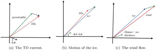measures the relative size of the contribution from the Ekman stress and the variation in ice thickness. For information, the vectors that describe the TD current, the motion of the ice and of the wind are depicted in figure 3. With the choice of geostrophic flow and Ekman contributions as shown in these figures, we have the wind to the right of the ice-motion and moving faster than the ice; correspondingly, the ice moves to the right of the Transpolar Drift current and at a speed greater than that of the near-surface current. Furthermore, the surface Ekman flow (shown in the first panel) is pointed in the general direction of Greenland, in agreement with the data presented in (Ma et al. 2017). In all these figures we see, for a reasonably large geostrophic flow, that this dominates the speeds and directions of the various elements that make up the wind-ice-ocean complex.

Figure 3. From left to right: (a) the geostrophic and Ekman flows producing the TD current (TDc); (b) the motion of the ice relative to the TDc; (c) the wind flow over the ice, relative to the direction of the ice.

Let us first consider the case of constant vectors for both the geostrophic flow and the Ekman flow; from (38(38) $\begin{array}{rl}{u}_i& =u_0-\frac{b}{m}(y+\mathrm{mx})+a(x,y)\cos (-\mathrm{k\pi })+{\nu }_i\sqrt{a(x,y)}\cos (\frac{\pi }{4}-\mathrm{k\pi }),\end{array}$(38) )-(39(39) $\begin{array}{rl}{v}_i& =v_0+b(y+\mathrm{mx})+a(x,y)\sin (-\mathrm{k\pi })+{\nu }_i\sqrt{a(x,y)}\sin (\frac{\pi }{4}-\mathrm{k\pi }).\end{array}$(39) ) we have seen that the motion of the ice is then also described by a constant vector. The solution for the ice thickness, obtained from equation (31(31) $\begin{array}{r}{c}_{\mathrm{oi}}=C_{\mathrm{oi}}\frac{{\rho }^{\prime }{U}^{\prime }{D}^{\prime }}{{\mu }^{\prime }},c_{\mathrm{oi}}=C_{\mathrm{ai}}\frac{{\rho }^{\prime }{U}^{\prime }{D}^{\prime }}{{\mu }^{\prime }},r_a=\frac{{\rho }_a^{\prime }}{{\rho }^{\prime }},\alpha =\frac{{\mathrm{\Pi }}^{\prime }{H}^{\prime }{D}^{\prime }}{R^{\prime }{U}^{\prime }{\mu }^{\prime }},\Gamma =\frac{{\Gamma }^{\prime }{R}^{\prime }}{U^{\prime }{H}^{\prime 2}},\end{array}$(31) ), follows directly: (42) $h=\sqrt{\frac{2\Gamma }{u_i}x+F(y-\frac{v_i}{u_i}x)},$(42) where F is an arbitrary function; this corresponds to the solution for thin ice given in Spall (2019). Because the ice moves in the direction given by $\arctan (\frac{v_i}{u_i})$, along these lines we have $F=\mathrm{constant}$ and consequently we cannot have a solution with decreasing thickness in the direction of motion; indeed, the thickness increases, as found in Spall (2019). Choosing to continue with our model for the boundary condition at the surface, the possibility that the ice thickness decreases will arise only if the motion of the ice is described by a variable vector. A natural way to accomplish this is to allow the geostrophic flow to vary in speed, which is already accommodated by our choice given in (32(32) $\begin{array}{rl}{u}_g& =\frac{\mathrm{\partial }\psi }{\mathrm{\partial }y}=u_0-\frac{b}{m}(y+\mathrm{mx}),\end{array}$(32) )-(33(33) $\begin{array}{rl}{v}_g& =-\frac{\mathrm{\partial }\psi }{\mathrm{\partial }x}=v_0+b(y+\mathrm{mx}),\end{array}$(33) ). Indeed, we note that the Transpolar Drift current certainly accelerates towards the Fram Strait but we will, for simplicity in this investigation, elect to use an Ekman component that moves at constant speed at the surface, i.e. $a=\mathrm{constant}$. The general solution of equation (31(31) $\begin{array}{r}{c}_{\mathrm{oi}}=C_{\mathrm{oi}}\frac{{\rho }^{\prime }{U}^{\prime }{D}^{\prime }}{{\mu }^{\prime }},c_{\mathrm{oi}}=C_{\mathrm{ai}}\frac{{\rho }^{\prime }{U}^{\prime }{D}^{\prime }}{{\mu }^{\prime }},r_a=\frac{{\rho }_a^{\prime }}{{\rho }^{\prime }},\alpha =\frac{{\mathrm{\Pi }}^{\prime }{H}^{\prime }{D}^{\prime }}{R^{\prime }{U}^{\prime }{\mu }^{\prime }},\Gamma =\frac{{\Gamma }^{\prime }{R}^{\prime }}{U^{\prime }{H}^{\prime 2}},\end{array}$(31) ), for h, is (43) $h=\sqrt{\frac{\Gamma (y+\mathrm{mx})}{V_i+m{U}_i}+G(\zeta ))},$(43) where $\begin{array}{rl}{U}_i& =u_0+a\cos (-\mathrm{k\pi })+{\nu }_i\sqrt{a}\cos (\frac{\pi }{4}-\mathrm{k\pi }),\\ V_i& =v_0+a\sin (-\mathrm{k\pi })+{\nu }_i\sqrt{a}\sin (\frac{\pi }{4}-\mathrm{k\pi }),\end{array}$ both constants, and G is an arbitrary function of (44) $\zeta =(V_i+m{U}_i)x+\frac{m}{2b}(U_i-\frac{b(y+\mathrm{mx})}{m}{)}^2.$(44) The natural way to proceed, even with all the simplifying assumptions that we have used thus far – we will comment on the relaxation of these later – is to choose an initial profile for the ice thickness along some line. However, to find a suitable form which produces the observed reduction in ice thickness as the flow travels from the North Pole towards the Fram Strait is not a trivial exercise. We therefore opt for a simple choice of $G(\zeta )$, namely linear in ζ, and impose an ice thickness that decreases (from $h_0$ to $h_1$) along the line given by the flow direction at the North Pole. This, in turn, produces an explicit description of the ice thickness which is needed in the expression for the wind velocity (see (40(40) $\begin{array}{rl}{u}_a& =u_i+{\nu }_a\sqrt{\frac{a(x,y)\cos ({\displaystyle \frac{\pi }{4}-\mathrm{k\pi })+\alpha \sqrt{2}\frac{\mathrm{\partial }h}{\mathrm{\partial }x}}}{\sqrt{1+{\beta }^2}}},\end{array}$(40) )-(41(41) $\begin{array}{rl}{v}_a& =v_i+{\nu }_a\sqrt{\frac{a(x,y)\sin ({\displaystyle \frac{\pi }{4}-\mathrm{k\pi })+\alpha \sqrt{2}\frac{\mathrm{\partial }h}{\mathrm{\partial }y}}}{\sqrt{1+{\beta }^2}}},\end{array}$(41) )); using this, we may find the wind speed. This variation in ice thickness is, of course, not driven by the physics, being prescribed by the need for a simple mathematical structure; other, more realistic choices, can be the subject of future studies.

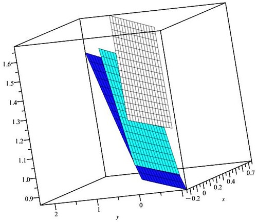
In figure 4 we show an example (computed using Maple) of the ice thickness, as a surface in a band about the line which represents the direction of the ice flow across the North Pole; this is valid only in the neighbourhood of the North Pole. This depicts a reduction in thickness in the direction of motion (from y = −0.5 to y = 1.2 in our nondimensional variables), together with an associated thickness-distribution of the initial profile (i.e. along a line through y = −0.5). This profile is consistent with a linear variation for $G(\zeta )$ and the imposed reduction in ice thickness along the flow. In figure 5 the speeds of the three elements that comprise the motion – the wind, the ice and the near-surface ocean – are shown, based on the choices made for the geostrophic flow and the ice thickness. This figure presents the speeds, as surfaces, aligned with the directions of motion at the North Pole. Thus the wind is fastest, and to the right of the motion of the ice, and the ice moves faster than the near-surface ocean flow and to the right of it. These calculations were performed using Maple, with the parameter choices $\begin{array}{rl}& u_0=0.3,v_0=1,k=0.1667,b=0.1,m=4,\\ & a=0.1,{\nu }_a=0.8,{\nu }_i=0.1,\alpha \sqrt{2}=0.01,\Gamma =0.1,\end{array}$ with $h_0=1$, $h_1=0.1$, and all plots are bounded by the lines y = −0.5 + mx and $y=1.5+\mathrm{mx}$ for $x\in [-0.25,0.75]$, where m is the direction of the flow – wind or ice or ocean – at the North Pole.

Figure 4. Ice thickness, showing the reduction from left to right (y = −0.5 to y = 1.2).

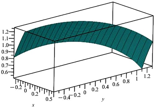
Figure 5. The speeds (on the vertical coordinate) and orientations of the wind (white), ice (cyan) and ocean (blue).

5. Discussion

We have presented a detailed description of the dynamics of the Transpolar Drift current, based on the appropriate governing equations valid in the neighbourhood of the North Pole, taken from (Constantin and Johnson 2023), combined with the thin-shell and f-plane approximations. This development has required the introduction of a suitable boundary condition (modelling the conditions at the surface) which represents the interaction between the wind, the ice and the near-surface ocean. As we have shown, there are choices of the various parameters which recover flow properties that are close to the general form that is observed: a decreasing thickness of ice as it flows towards the Fram Strait, with associated wind, ice and ocean movement.

The solution as presented allows for many adjustments to the various flow conditions, controlling the speed, direction and variability of each of the three components. Although, we argue, the underlying governing equations (valid at and near the North Pole), combining the thin-shell and f-plane approximations, are essentially fixed, the choice of the surface stress model and the ambient flow conditions is flexible. Here, we opt for a simplified version of the boundary condition describing the interaction of the wind, the ice and the ocean, this based on the seminal work of Hibler (1979) (and refined by Spall 2019), but with a stress proportional to the square of the relative speed. Clearly, this model could be improved (or replaced altogether), but at the expense – probably – of complications in the analysis. However, since we appear to have captured all the relevant stress conditions, this suggests that not much will be gained by changing the model that describes the stresses in the surface boundary condition. Further, this approach allows for the initial profile of the ice thickness to be given along some initial line. Of far greater significance is the balance between the choices for the background flow (geostrophic and wind) and their relative magnitudes and directions.

Our approach admits very considerable freedom in the choices for the near-surface geostrophic flow and the wind that drives the motion from above. It is this aspect of the problem which, particularly when based on reliable data, requires further analysis and investigation. Thus we may start with any suitable geostrophic, near-surface flow which can move in a prescribed (but variable) direction with a variable speed, represented as a function of $(x,y)$ in our formulation. Further, the near-surface wind which drives the motion from above can be prescribed in a similar fashion. This will, via the surface stress conditions, drive the ice and, correspondingly, produce a stress at the surface of the ocean which produces the associated variable Ekman flow; the combination of this with the geostrophic flow gives the Transpolar Drift current. Although, for the ease of presentation, we have opted to calculate up from the ocean by assuming a simple form for the Ekman component, leading to the wind consistent with this solution, it is evident that a unique solution exists, given the wind and the geostrophic flow. And there is one other obvious extension of this work: to retain the spherical geometry, but within the thin-shell approximation, and so aim to find a solution which is valid as far as, and possibly beyond, the Fram Strait. We submit, therefore, that we have put in place an accessible description of the dynamics of the Transpolar Drift current which can be used to test various hypotheses and to investigate the rôle of chosen background flows (wind and ocean), particularly when based on accurate data.

Acknowledgments

All data for this paper are properly cited and referred to: the relevant data can be found in Morison and McPhee (2001), Haller et al. (2014), Ma et al. (2017), Kwok (2018), Morison et al. (2018), Morison et al. (2021), Wilson et al. (2021), Jin et al. (2023), and Ward and Tandon (2024). The authors are grateful for helpful comments from the referee.

Disclosure statement

No potential conflict of interest was reported by the author(s).

Additional information

Funding

This research was supported by the Austrian Science Fund (FWF) [grant number Z 387-N].

References

- Charette, M.A., Kipp, L.E., Jensen, L.T., Dabrowski, J.S., Whitmore, L.M., Fitzsimmons, J.N., Williford, T., Ulfsbo, A., Jones, E., Bundy, R.M., Vivancos, S.M., Pahnke, K., John, S.G., Xiang, Y., Hatta, M., Petrova, M.V., Heimbürger-Boavida, L.-E., Bauch, D., Newton, R., Pasqualini, A., Agather, A.M., Amon, R.M.W., Anderson, R.F., Andersson, P.S., Benner, R., Bowman, K.L., Edwards, R.L., Gdaniec, S., Gerringa, L.J.A., González, A.G., Granskog, M., Haley, B., Hammerschmidt, C.R., Hansell, D.A., Henderson, P.B., Kadko, D.C., Kaiser, K., Laan, P., Lam, P.J., Lamborg, C.H., Levier, M., Li, X., Margolin, A.R., Measures, C., Middag, R., Millero, F.J., Moore, W.S., Paffrath, R., Planquette, H., Rabe, B., Reader, H., Rember, R., Rijkenberg, M.J.A., Barman, M.R., Rutgers van der Loeff, M., Saito, M., Schauer, U., Schlosser, P., Sherrell, R.M., Shiller, A.M., Slagter, H., Sonke, J.E., Stedmon, C., Woosley, R.J., Valk, O., van Ooijen, J. and Zhang, R., The transpolar drift as a source of riverine and shelf-derived trace elements to the central Arctic Ocean. J. Geophys. Res.: Oceans 2020, 125, e2019JC015920.
- Constantin, A., Comments on: Nonlinear wind-drift ocean currents in arctic regions. Geophys. Astrophys. Fluid Dyn. 2022a, 116, 116–121.
- Constantin, A., Nonlinear wind-drift ocean currents in arctic regions. Geophys. Astrophys. Fluid Dyn. 2022b, 116, 101–115.
- Constantin, A. and Johnson, R.S., Ekman-type solutions for shallow-water flows on a rotating sphere: a new perspective on a classical problem. Phys. Fluids 2019, 31, 021401.
- Constantin, A. and Johnson, R.S., On the modelling of large-scale atmospheric flows. J. Differ. Equations 2021, 285, 751–798.
- Constantin, A. and Johnson, R.S., On the dynamics of the near-surface currents in the Arctic Ocean. Nonlinear Anal. Real World Appl. 2023, 73, 103894.
- Constantin, A. and Johnson, R.S., Spherical coordinates for Arctic Ocean flows. In Nonlinear dispersive equations, edited by D. Henry, 2024 (Springer: Cham).
- Gascard, J.-C. and Metaxian, J.-P., Exploring Arctic transpolar drift during dramatic sea ice retreat. EOS 2008, 89, 21–28.
- Haller, M., Brümmer, B. and Müller, G., Atmosphere-ice forcing in the transpolar drift stream: results from the DAMOCLES ice-buoy campaigns 2007–2009. The Cryosphere 2014, 8, 275–288.
- Hibler, W.D., A dynamic-thermodynamic sea-ice model. J. Phys. Oceanogr. 1979, 9, 815–846.
- Jin, Y., Chen, M., Yan, H., Wang, T. and Yang, J., Sea level variation in the Arctic Ocean since 1979 based on ORAS5 data. Front. Mar. Sci 2023, 10, 1197456.
- Johnson, R.S., The ocean and the atmosphere: an applied mathematician's view. Comm. Pure Appl. Anal. 2022, 21, 2357–2381.
- Johnson, R.S., An Introduction to The Mathematical Fluid Dynamics of Oceanic and Atmospheric Flows, 2023 (Berlin: EMS Press).
- Kwok, R., Arctic sea ice thickness, volume, and multiyear ice coverage: losses and coupled variability (1958–2018). Environ. Res. Lett. 2018, 13, 105005.
- LeBlond, P.H., Planetary waves in a symmetrical polar basin. Tellus 1964, 16, 503–512.
- Leppäranta, M., The Drift of Sea Ice, 2011 (Berlin: Springer).
- Ma, B., Steele, M. and Lee, C.M., Ekman circulation in the Arctic Ocean: beyond the Beaufort Gyre. J. Geophys. Res.: Oceans 2017, 122, 3358–3374.
- Morison, J., Kwok, R., Dickinson, S., Andersen, R., Peralta-Ferriz, C., Morison, D., Rigor, I., Dewey, S. and Guthrie, J., The cyclonic mode of arctic ocean circulation. J. Phys. Oceanogr. 2021, 51, 1053–1075.
- Morison, J.H. and McPhee, M., Ice-ocean interaction. In Encyclopedia of Ocean Sciences, edited by J. Steele, pp. 1271–1281, 2001 (Academic Press: New York).
- Morison, J., Wilkinson, J., Alkire, M., Nilsen, F., Polyakov, I., Smethie, W., Schlosser, P., Vivier, F., Lourenco, A., Provost, C., Pelon, J., Ferriz, C. P., Karcher, M., Rabe, B. and Lee, C., The North Pole region as an indicator of the changing Arctic Ocean. Arctic 2018, 71, 1–15.
- Nof, D., Modons and monopoles on a Γ-plane. Geophys. Astrophys. Fluid Dyn. 1990, 50, 71–87.
- Olason, E. and Notz, D., Drivers of variability in Arctic sea-ice drift speed. J. Geophys. Res. Oceans 2014, 119, 5755–5775.
- Serreze, M.C. and Barry, R.G., The Arctic Climate System, 2014 (Cambridge: Cambridge University Press).
- Spall, M.A., Dynamics and thermodynamics of the mean transpolar drift and ice thickness in the Arctic Ocean. J. Climate 2019, 32, 8449–8463.
- Talley, L.D., Pickard, G.L., Emery, W.J. and Swift, J.H., Descriptive Physical Oceanography: An Introduction, 2011 (Amsterdam: Elsevier).
- Thomas, J.H. and Lux, R.A., Refraction of Rossby waves on a multiple β-plane. Dyn. Atmos. Oceans 1978, 2, 411–426.
- Timmermans, M.-L. and Marshall, J., Understanding Arctic Ocean circulation: a review of ocean dynamics in a changing climate. J. Geophys. Res.: Oceans 2020, 125, e2018JC014378.
- Vallis, G.K., Atmospheric and Oceanic Fluid Dynamics, 2005 (Cambridge: Cambridge University Press).
- Wadhams, P., Ice in The Ocean, 2014 (London: CRC Press).
- Ward, J.L. and Tandon, N.F., Why is summertime Arctic sea ice drift speed projected to decrease? The Cryosphere 2024, 18, 995–1012.
- White, A.A., A view of the equations of meteorological dynamics and various approximations. In Large-scale Atmosphere-Ocean Dynamics, edited by J. Norbury and I. Roulstone, pp. 1–100, 2002 (Cambridge: Cambridge University Press).
- Wilson, C., Aksenov, Y., Rynders, S., Kelly, S.J., Krumpen, T. and Coward, A.C., Significant variability of structure and predictability of Arctic Ocean surface pathways affects basinwide connectivity. Commun. Earth Environ. 2021, 2, 164.
- Yang, H., Evolution of a Rossby wave packet in barotropic flows with asymmetric basic current, topography and ε-effect. J. Atmos. Sci. 1987, 44, 2267–2276.