The pickup and delivery problem with time windows and scheduled lines

ABSTRACT

Integrating freight flows with scheduled public transportation services creates attractive business opportunities as the same transportation needs can be met with fewer operating costs. The pickup and delivery problem with time windows and scheduled lines (PDPTW-SL) aims at routing a given set of vehicles to transport freight requests from their origins to their corresponding destinations, where the requests can use scheduled passenger transportation services as a part of their journeys. We describe the PDPTW-SL as an arc-based mixed-integer program. Computational results on a set of small-size instances provide a clear understanding of the benefits of using scheduled line services as a part of freight's journey.

KEYWORDS:

• Freight transportation
• multi-modal transportation
• routing and scheduling
• scheduled lines

1. Introduction

A successful integration of freight and public transportation creates a seamless movement for both people and goods (i.e. small parcels). Actual integration is already being observed in long-haul freight transportation (Levin et al. 2012). For example, Norwegian Hurtigruten carries freight and people at the same time (Hurtigruten 2013). In short-haul transportation, however, people and freight rarely share transportation modes although they largely use the same infrastructure (Lindholm & Behrends 2012). Knowing this reality, potential efficiency gains for an integrated approach can be further investigated. To the best of our knowledge, integrated transport solutions to short-haul transportation have not been sufficiently taken into consideration in the literature.

This paper focuses on opportunities to make use of available public transportation, which operates according to predetermined routes and schedules, as a part of freight journey. We assume that each considered public transport vehicle has a finite carrying capacity for freight requests apart from available spaces destined for passengers. Therefore, transferring freight requests to available scheduled lines (SLs) could be beneficial for the whole transportation system. We consider two transport options: direct and indirect shipments. The first one implies that origin and destination points of a request are visited by using only one pickup and delivery (PD) vehicle. On the other hand, the second type of shipment implies that a request is picked up by a PD vehicle and transferred to a transfer node, which is assumed to be located nearby. From there, the request continues its journey on SLs. Afterwards, the request is picked up again by another PD vehicle to be delivered to its destination point. In this paper, we denote this specific transportation problem as the pickup and delivery problem with time windows and scheduled lines (PDPTW-SL). A schematic overview of the example network is shown in Figure 1.

Figure 1. An illustration of the integrated transportation network.

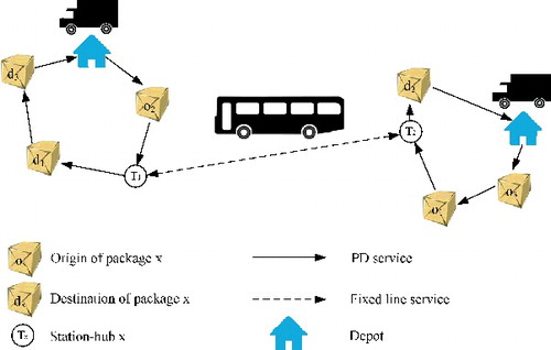
Figure 1 presents three requests that have their PD locations close to two different transfer nodes. It would make sense to use a SL that connects these two transfer nodes instead of using one PD vehicle as in the pickup and delivery problem (PDP). Hence, travel time savings of PD vehicles and operational cost reduction can be expected with the proposed integrated system.

It is noteworthy that a small-sized freight (i.e. packages) is considered and the consolidation of the requests is done on both modes of transportation. In other words, a PD vehicle can perform several pickups before it delivers the requests to their delivery nodes, hence, carrying larger quantities. Similarly, SLs facilitate for consolidation in the start node, thus multiple freight requests can be transported on the SL vehicles at a time (as long as the capacity constraint is not violated). Hence, freight consolidation leads to higher efficiency of the whole transportation system.

The contributions of the paper are the following: (1) we introduce a mixed-integer program for the PDPTW-SL, (2) we propose some effective valid inequalities for the given formulation and (3) we analyse the benefits of using SLs in a PD environment by comparing the solutions of the PDPTW with the solution of the PDPTW-SL. The remainder of the paper is structured as follows. Section 2 provides a brief review of the related works. Section 3 introduces a mixed-integer programming (MIP) formulation for the PDPTW-SL. Section 4 reports the results obtained from extensive computational experiments. Section 5 provides conclusions and future research directions.

2. Literature review

This section reviews the literature addressing the related problems of the PDPTW-SL. To the best of our knowledge, there is only limited literature on transfer options to SL services. Thus, our paper is one of the first attempts to investigate integrated short-haul freight transportation from an operational planning perspective.

In the context of PDP, we refer to Berbeglia et al. (2007) for a literature survey on solution methodologies. Cordeau and Laporte (2007) provide an overview of mathematical models and solution methodologies for single- as well as multi-vehicle dial-a-ride problem (DARP), which is an extension of the PDP. In a related study by Parragh (2010), the author investigates heterogeneity in vehicles and passengers along with waiting times of passengers. The author proposes a Branch & Cut (B&C) and a variable neighbourhood search (VNS) algorithm to solve the DARP. Parragh et al. (2012) extend the heterogeneous DARP to consider driver-related constraints and propose a hybrid column generation and VNS heuristic algorithm.

One of the PDP extensions considering transfer opportunity between PD vehicles at transfer nodes is coined as PDP with transfers (PDP-T). In the PDP-T, a request can be picked up by one vehicle and delivered by another. A relevant study by Shang and Cuff (1996) is one of the earliest works on the PDP-T. The authors propose an insertion heuristic algorithm which leads to a cost reduction of up to 37% compared to the manual plans. In the work of Cortes et al. (2010), the authors propose an exact decomposition method, namely B&C, to solve the PDP-T. The proposed algorithm provides savings of up to 90% in terms of CPU time compared to traditional Branch & Bound (B&B) algorithm. In another work, Masson et al. (2012) introduce an adaptive large neighbourhood search (ALNS) algorithm to solve the PDP-T. Their results indicate savings of up to 9% in terms of travel time, obtained by using intermediate transfers. In addition, Masson et al. (2014) propose an ALNS for the DARP with transfers (DARPT). The authors show that using transfers between vehicles may lead to significant savings in terms of operating costs (i.e. up to 8%). In addition, Petersen and Røpke (2011) investigate the PDP with cross-docking opportunities (PDPCD). The authors propose a large neighbourhood search heuristic for the PDPCD. Their results suggest that improvements of up to 5% can be achieved due to cross-docking operations.

One of the first authors that conceptually introduced the idea of transporting freight using public transport was Nash (1982). Later, Liaw et al. (1996) investigate the opportunity to integrate SL services with the DARP. The authors formulate the problem where transshipment to public scheduled transportation is allowed for passengers and wheel-chaired persons and propose two types of heuristics (i.e. online and offline). Their computational results show that improvements of up to 9% in terms of the number of serviced requests can be obtained using static planning and up to 7% with the help of online decision support. In another work, Aldaihani and Dessouky (2003) consider an integrated DARP with public transport and propose a two-stage heuristic algorithm (i.e. insertion and tabu search). Computational results indicate that solutions generated by the proposed algorithm lead to cost savings of 16.6%. In a related work of Häll et al. (2009), the authors introduce a MIP formulation to solve an integrated DARP. The authors consider transfers to fixed lines without modelling the schedule of the public transportation.

Trentini and Malhene (2010) study an overview of solutions for combining freight and passenger transportation that are used in practice. The authors divide transport solutions into three categories: shared road capacities (multi-use lanes, night deliveries, etc.), shared public transport services (buses, subway, etc.) and, finally, shared consolidation facilities (delivery bays, lockers, etc.). In a related study, Trentini et al. (2012) investigate a two-echelon vehicle routing problem with transshipment in the context of public and freight integrated transportation system. The authors propose to use public transportation to ship the goods from a central distribution centre to predefined stations (e.g. transshipment points). From there, a number of tricycles are used to deliver products to their final destinations. The authors propose ALNS along with a MIP formulation. Based on their results, the integrated solution proved to be more efficient in terms of pollution compared to traditional routing.

Table 1 provides an overview of the most relevant literature. We note that all papers in the table consider time window (TW) aspect.

Table 1. An overview of the related literature.

				Transfers to fixed lines
Research	Multi-depots	Hetero-geneous fleet	Transfers among PD vehicles	No sched.^a	Sched.^b	Dyna-mics	Solution approach
Shang and Cuff (1996)	–	–	✓	–	–	–	Heuristic
Cortes et al. (2010)	✓	✓	✓	–	–	–	B&C
Masson et al. (2012)	–	–	✓	–	–	–	Metaheuristic
Masson et al. (2014)	✓	–	✓	–	–	–	Metaheuristic
Liaw et al. (1996)	–	–	–	–	✓	✓	Heuristic
Häll et al. (2009)	–	–	–	✓	–	–	B&B
Trentini et al. (2012)	–	–	–	–	✓	–	Metaheuristic
This paper	✓	✓	–	–	✓	–	B&B

^aTime schedules of the fixed lines are not considered.

^bTime schedules of the fixed lines are considered.

‘–’: the aspect is not considered.

‘✓’: the aspect is considered.

As seen in Table 1, the literature on SL services is limited. Therefore, we aim at creating a building block for further research in this area, considering the extra complexity due to integrating SLs with current road transport flows.

3. Mathematical formulations for the PDPTW-SL

In this section, we introduce a MIP formulation for the PDPTW-SL. All information (requests, demands, travel times and TWs) is assumed to be known in advance and an initial plan for the whole planning horizon (e.g. one day) is generated. More specifically, the plan is generated before operating day commences by considering only the requests known at the moment of planning (i.e. static planning). A solution to our model is a routing plan for the PD vehicles such that each request is served. Additionally, a time schedule for the PD vehicles and to-be-served requests is produced. The aim is to minimize the total operating costs. These include (1) operating (routing) cost of the PD vehicles and (2) the total transfer cost which is proportional to the number of shipped requests on the SLs.

3.1. Definitions and assumptions

We define the PDPTW-SL on a digraph = (, ), where represents the set of nodes and represents the set of arcs. All other definitions and assumptions are described below.

Requests. Every request r involves a pickup node r and a delivery node r + n, with n being the total number of requests that need to be services. In addition, any request r has two required TWs: one for the pickup node ([l_r, u_r]) and one for the delivery node ([l_{r + n}, u_{r + n}]). The set of all requests is provided as . Note that we refer to a request by referring to its corresponding pickup node. Finally, demand d_r is known for each request.

PD vehicles. The set includes all available PD vehicles. Furthermore, Q_v corresponds to the carrying capacity of PD vehicle v. The origin and destination of every PD vehicle is given as node o_v with its TW [, ].

Travelling and service times. Travelling times, along with service times are assumed to be static and deterministic. Constant ϒ_ij represents the travel time from node i to node j. In addition, parameter s_i corresponds to the service time at node i ∈ .

Scheduled lines. Set contains all physical transfer nodes (i.e. end-stations of the SLs). Therefore, represents the set of all physical SLs. Each SL (i, j) connects the end-stations such that i, j ∈ . From the modelling perspective, note that arcs (i, j) and (j, i), i, j ∈ , represent two SLs. Each fixed line (i, j) has a set of indices for the scheduled departures from node i, such that p^w_ij represents the departure time, ∀ (i, j) ∈ , w ∈ . Note that each SL may have different frequency than other lines, thus the size of may differ. Furthermore, it is assumed that SL vehicles are designed to carry a limited amount of packages, thus implying a finite carrying capacity k_ij, ∀ (i, j) ∈ . It is assumed that package carrying capacity is not influenced by the passenger demand.

Each physical transfer node is assumed to be a consolidation location for the packages (e.g. DHL-Packstation 2013). Namely, a secured area for temporary storage of the packages is available. The packages can be stored until their departure time (either by fixed line or PD vehicle) at these stations. Furthermore, as multiple freight carriers may be using SL services, we assume that each carrier is assigned a part of the storage at the transfer nodes and SL vehicles capacity (e.g. contract-based agreement). Hence, the considered capacity is not affected by the demand of another actors involved. In addition, it is also assumed that cost η_ij per each unit of parcels shipped on the SL (i, j) includes transportation, handling (transshipment) and storage costs. Handling of the packages is assumed to be the responsibility of the SL service provider (e.g. a driver of the SL vehicle). Additionally, as the focus of the present problem is on the operational aspects, we disregard all investments needed, e.g. re-design of the SL vehicles and storage facilities at transfer nodes.

For modelling purposes, each physical SL (i, j) ∈ (e.g. arcs (1, 2) and (2, 1) in the example shown in Figure 2(a)) gets n replications as in Häll et al. (2009). This is done to consider multiple visits and waiting times of the PD vehicles at the transfer nodes. In addition, each replication is assigned to one request, and only that specific request can be shipped on the assigned SL (refer to Figure 2(b)). Therefore, contains all replicated SLs (e.g. arcs (1a, 2a), (1b, 2b), (2a, 1a) and (2b, 1b) in Figure 2(b)).

Figure 2. An example of a replicated scheduled line. (a) Physical scheduled line and (b) virtual scheduled line.

As a consequence, every physical transfer node in (e.g. nodes 1 and 2 in Figure 2(a)) gets n replications, thus obtaining the set of replicated transfer nodes as (e.g. ≡ {1a, 1b, 2a, 2b} in Figure 2(b)). For modelling purposes, let ψ^t, ∀ t ∈ show the physical transfer node represented by t (e.g. ψ^1a = ψ^1b = 1). Consequently, can be defined as , ∀ t ∈ (e.g. in Figure 2(b), = {2b}, as 2a and 2b represent physical transfer node 2). Note that ⊂ , ∀ t ∈ .

The proposed model can consider any complex SL network topology. Thus, we also assume that the requests can be transferred from one SL to another. Table 2 shows the parameters used in our model.

Table 2. Parameters.

Notation	Definition
δ	Number of depots
ϒij	Travelling time from node i to node j
si	Service time at node i
kij	Package carrying capacity on the fixed line (i, j)
[li, ui]	Time window at node i
p^wij	Departure time from node i, on the fixed line (i, j), indexed by w
τ	The amount of replicated transfer nodes (i.e. )
f^ri	(see Table 3)
φv	The routing cost of one time unit for vehicle v
ηij	The cost of shipping one unit of parcel on the SL (i, j)
Qv	Freight carrying capacity of vehicle v

The sets can be represented as in Table 3.

Table 3. Sets.

Notation	Definition
	Set of depots, ≡ [1, ..., δ] (i.e. ov ∈ , ∀ v ∈ )
	Set of requests (pickup nodes), ≡ [δ + 1, …, δ + n]
	Set of delivery nodes, ≡ [δ + n + 1, …, δ + 2n]
	Set of replicated transfer nodes, ≡ [δ + 2n + 1, …, δ + 2n + τ](e.g. nodes 1a, 1b, 2a and 2b in Figure 2(b))
	Set of replicated transfer nodes that represent the same physical transfer node as t (e.g. in Figure 2(b), = {2b}, = {1b}, etc.)
	Set of nodes in ; ∪ ∪ ∪ ≡
	∪
	∪ ∪
	Set of PD vehicles
	Set of physical fixed lines which is defined as (i, j) with associated and kij
	Set of indices for the departure times from the physical transfer node i on fixed line (i, j) ∈
	Set of replicated fixed lines which is defined as (i, j) with associated
	Set of replicated fixed lines associated with request r (e.g. in Figure 2 = {(1a, 2a), (2a, 1a)})
	Set of replicated fixed lines connected to the replicated transfer node t (e.g. in Figure 2, = {(1a, 2a), (2a, 1a)})
	Set of replicated fixed lines associated with a physical fixed line (i, j) ∈ (e.g. in Figure 2, = {(1a, 2a), (1b, 2b)}, = {(2a, 1a), (2b, 1b)})
	Set of arcs in defined by × , (note that ∖ ≡ ∪ ∪ )
	= × ∖

Table 4 shows the decision variables used in the proposed formulation.

Table 4. Decision variables.

Notation	Definition
x^vij	A binary variable with value 1 if arc (i, j) is traversed by PD vehicle v, 0 otherwise, ∀ (i, j) ∈ , v ∈
αv	A continuous variable that indicates the time vehicle v returns to its depot, ∀ v ∈
βi	A continuous variable that indicates the departure time of a PD vehicle from node i, ∀ i ∈
y^rij	A binary variable with value 1 if arc (i, j) is traversed by request r, 0 otherwise, ∀ i, j ∈ , r ∈
γ^ri	A continuous variable that indicates the departure time of request r from node i, ∀ i ∈ , r ∈
q^rwij	A binary variable with value 1 if replicated SL (i, j) is used by request r that departs from i at time p^wij, 0 otherwise, ∀ r ∈ , (i, j) ∈ , w ∈

3.2. An arc-based formulation

The PDPTW-SL is formalized as an arc-based MIP, as follows:(1) Term (1(1) ) minimizes the total travel cost of the PD vehicles and the cost of using SLs for the transferred requests.

subject to

The routing and flow constraints(2) (3) (4) (5) (6) (7) (8)

In the first block of constraints, (2(2) ) assure that all PD nodes are visited exactly once. Constraints (3(3) ) make sure that each considered PD vehicle is used at most once, and constraints (4(4) ) avoid visiting each replicated transfer node more than once. Flow balance for the PD vehicles is assured by constraints (5(5) ). Constraints (6(6) ) enforce flow balance for each request. Constraints (7(7) ) assure that a PD vehicle should pick up/drop off a request at a replicated transfer node related to a SL, if there is a flow on this specific SL. Constraints (8(8) ) force the capacity of each PD vehicle.

The scheduling constraints(9) (10) (11) (12) (13) (14) (15) (16) (17)

Timing for each request is considered in constraints (9(9) ). Similarly for PD vehicles, scheduling is updated in constraints (10(10) ) and (11(11) ). Constraints (12(12) ) assure the precedence constraints, and constraints (13(13) ) and (14(14) ) enforce the TWs. Constraints (15(15) ) and (16(16) ) assure the scheduling of the available SLs. Constraints (17(17) ) make sure that the package carrying capacity on the SL is not exceeded.

The synchronisation constraints(18) (19) (20) (21)

Time synchronization between requests and PD vehicles is considered in constraints (18(18) )–(21(21) ). For clarity reasons, we present constraints (9(9) )–(11(11) ), (16(16) ) and (18(18) )–(21(21) ) as implications. However, well-known big-M technique can be used to linearize these constraints.

Decision variable domains(22) (23) (24) (25) (26) (27)

Since PDPTW-SL is an extension of the PDPTW, it is an non-deterministic polynomial-time (NP)-hard problem. We also note that an optimal solution for the PDPTW represents an upper bound for the PDPTW-SL because the opportunity of using SLs does not restrict the option of direct shipping. The complexity of the PDPTW-SL based on its input is as follows:

• ), if ≥ n,

• ), if < n.

On the other hand, the complexity of the PDPTW based on its input is O(). It is noted that = and in most of the cases n > . Hence, the complexity of the PDPTW-SL is greater than or equal to the complexity of the PDPTW (i.e. O(PDPTW-SL) ≥ O(PDPTW)).

Considering the explosion in complexity along with the increase in instance size, a certain preprocessing needs to be implemented in order to reduce the size of the network. The subsequent section will introduce several elimination rules.

3.2.1. Preprocessing

A preprocessing was implemented in order to reduce the number of decision variables. Hence, some of the infeasible arcs in graph are removed.

• A vehicle cannot leave from and return to a depot other than its own.

• No vehicle can travel from the destination to the origin of the same request.

• No PD vehicle can travel between nodes i and j, if (i, j) ∈ .

• No request r can travel between origin and destination of a fixed line other than arc (i, j) ∈ .

• No request r can travel from the destination to the origin of the same request.

• No request is allowed to travel to/from any depot.

• No flow is allowed between nodes i and j, if l_i + s_i + ϒ_ij > u_j.

• No request can travel from its delivery node to any other node.

• No request can travel to its pickup node from any other node.

In addition, some elimination rules related to transfer nodes can be applied.

• An arc (t₁, t₂) is infeasible if l_r + s_r + + + + + > u_{r + n}, ∀ r ∈ , (t₁, t₂) ∈ .

The number of departure times on the SLs for each request can be reduced by considering the TWs. For example, no request r can depart at a time earlier than (l_r + s_r + + ) on the SL (t₁, t₂), ∀ r ∈ , (t₁, t₂) ∈ . Similarly, no request r can depart at a time later than (u_{r + n} – s_{r + n} – – – – ) on a SL (t₂, t₁), ∀ r ∈ , (t₂, t₁) ∈ .

3.2.2. Model tightening

As the proposed arc-based formulation grows very rapidly in size with the number of requests, number of SLs and departure times on each line, some additional constraints (valid inequalities) may be added to improve the formulation. This section introduces three sets of cuts (i.e. flow tightening, vehicle service tightening and depot strengthening) that are valid for the PDPTW-SL.

We state Proposition 3.1 for flow tightening as follows.

Proposition 3.1:

The following inequality is valid for the PDPTW-SL:(28)

Proof:

Let (i, j) ∈ A⁵. In addition, let x^v_ij, ∀ v ∈ , (i, j) ∈ and y^r_ij, ∀ r ∈ , i, j ∈ be binary variables. We consider two cases: (1) PD vehicle does not traverse (i, j) ∈ (i.e. = 0) and (2) PD vehicle travels on (i, j) ∈ (i.e. = 1).

In case (1), due to capacity constraints (8(8) ), no request can travel on (i, j) (i.e. y^r_ij = 0, ∀ r ∈ ). In case (2), any request can travel on (i, j) as long as constraints (8(8) ) are satisfied. Therefore, y^r_ij ∈ {0, 1}, ∀ r ∈ ensure that ≥ y^r_ij, ∀ r ∈ . □

Example 3.1:

Let there be a flow between i and j traversed by a vehicle v with its capacity equal to two units (i.e. Q_v = 2). In addition, two requests, r₁ and r₂, each having demand one (i.e. = = 1) travel on the same arc. Assume a linear programming (LP) relaxation solution with following values: x^v_ij = 0.2, = 0.3 and = 0.1. Hence, constraints (8(8) ) are satisfied (0.3 + 0.1 ≤ 2 × 0.2). By using constraints (28(28) ), x^v_ij is restricted to be at least 0.3 and = 0.3 and = 0.1, respectively. The resulting inequality is valid (0.3 + 0.1 ≤ 2 × 0.3).

A second proposition for vehicle service tightening is given in Proposition 3.2.

Proposition 3.2:

The following inequalities are valid for the PDPTW-SL:(29) (30)

Proof:

Let r ∈ and v ∈ . In addition, let x^v_ij, ∀ v ∈ , (i, j) ∈ and y^r_ij, ∀ r ∈ , i, j ∈ be binary variables. We consider three cases: (1) r is served by PD vehicle v; (2) r is served by two different PD vehicles, v and e.g. v₁ ∈ ; (3) r is served by other PD vehicle(s) v₁ and/or v₂ ∈ ;

In case (1), due to constraints (2(2) ), pickup ( = 1) and delivery nodes ( = 1) of r are visited by v, hence the left-hand side (LHS) of the constraints (29(29) ) and (30(30) ) take a value of zero. Furthermore, ≥ 0 ensures that even request r is served by v, it may still use a SL as part of its journey.

In case (2), the pickup or the delivery node of r is visited by v. Hence, LHS of constraints (29(29) ) and (30(30) ) may take two values: −1 and 1. In order to satisfy constraints (7(7) ), > 0, which implies that r must use a SL as part of its journey.

In case (3), PD vehicle v does not visit the pickup, nor the delivery node of r, thus LHS gets value zero. Hence, ≥ 0 guarantees that r can use a SL, as it may be served by one or two other PD vehicles. The result follows from these cases. □

A depot-related valid inequality is given in Proposition 3.3.

Proposition 3.3:

The following inequality is valid for the PDPTW-SL:(31)

Proof:

Let v ∈ and x^v_ij, ∀ v ∈ , (i, j) ∈ be binary variable. Assume that each vehicle starts and ends its operating day at its depot (i.e. o_v). We know that any node i ∈ cannot be visited before leaving the depot. Due to the timing constraints (10(10) ) and (11(11) ), this assumption holds and the departure of v from its depot should be smaller than the departure time from any other node. More specifically, if > 0, then gets a value of 1 ⇒ inequality (31(31) ) holds. □

Example 3.2:

Assume a part of an LP solution with two PD vehicles, namely v₁, v₂ ∈ and i, j ∈ and = = 0 (see Figure 3

Figure 3. An example of violation for constraint (31(31) ).

). This LP solution satisfies constraints (2(2) )–(21(21) ).

Constraints (31(31) ) ensure that > 0 and/or > 0. Thus, the LP solution given in Figure 3 violates constraints (31(31) ). In addition, note that M can be substituted by , which implies that a PD vehicle can visit each node in at most once.

4. Computational results

This section presents the results obtained from solving the proposed arc-based formulation of the PDPTW-SL using CPLEX. The model is implemented in NetBeans IDE 7.1.1 using the corresponding CPLEX 12.1 libraries. Furthermore, all experiments are run on a server with four CPU's (2.4 GHz/6 cores) and 32 GB RAM.

4.1. Instance description

We have generated three sets of instances with up to three SLs (triangular topology), namely R, C and RC, which differ in the geographical distribution of the request nodes. More specifically, C consists of nodes positioned within at most 30 time units to one of the available three transfer nodes whereas RC includes nodes within 80 time units, respectively, and R considers uniform-randomly distributed request nodes. The frequency of the SLs is one departure every 30 time units. Each instance contains up to 12 requests (i.e. 12 pickup and 12 delivery nodes) over 200×200 dimensional units on an Euclidean space. In these instances, one distance unit corresponds to one driving time unit, thus the longest trip between two locations would be approximately 4 hours. It would, therefore, represent a service area of a metropolis. Instances are named in format, where G is the geographic characteristic of the customer nodes, n is the amount of freight requests that need to be serviced, sl is the amount of available SLs and v is the amount of available PD vehicles. In all cases, two depots with up to three heterogeneous PD vehicles each are considered.

We assume a planning horizon of 600 time units (i.e. 10 working hours). The widths of the TWs are generated randomly with an average of 40 time units. Service times are assumed to be up to three time units. The demand of each request is randomly chosen between one and three units. The carrying capacities of PD vehicles is randomly generated between 16 and 20 units. The SL capacity is assumed to be 15 demand units. The instance sets are available on www.smartlogisticslab.nl.

Tables 5 and 6 present further details regarding instances. In each table, the column Instance shows the identification of the instance. Table 5 provides the number of depots (), the number of PD vehicles (), the number of requests (), the number of fixed lines () and their corresponding scheduled departure times. Table 6 provides the number of constraints, the number of variables in the resulting formulation, time to solve the LP relaxation and finally, objective function value of the LP relaxation. Corresponding values are computed with and without the proposed preprocessing in Section 3.2.1.

Table 5. Input sets.

Instance					·
C_6_1_4	2	4	6	2	36
C_7_1_4	2	4	7	2	36
C_8_1_4	2	4	8	2	36
C_9_1_4	2	4	9	2	36
C_10_1_4	2	4	10	2	36
C_11_1_4	2	4	11	2	36
C_12_1_4	2	4	12	2	36
RC_6_1_4	2	4	6	2	36
RC_7_1_4	2	4	7	2	36
RC_8_1_4	2	4	8	2	36
RC_9_1_4	2	4	9	2	36
RC_10_1_4	2	4	10	2	36
RC_11_1_4	2	4	11	2	36
RC_12_1_6	2	6	12	2	36
R_6_1_4	2	4	6	2	36
R_7_1_4	2	4	7	2	36
R_8_1_4	2	4	8	2	36
R_9_1_4	2	4	9	2	36
R_10_1_4	2	4	10	2	36
R_11_1_4	2	4	11	2	36
R_12_1_6	2	6	12	2	36

Table 6. The effect of preprocessing.

	No preprocessing						Preprocessing
	PDPTW-SL				PDPTW		PDPTW-SL				PDPTW
Instance	Cons	Vars	LP	CPU	Cons	Vars	Cons	Vars	LP	CPU	Cons	Vars
C_6_1_4	5208	5055	188.72	1.07	910	382	4363	4206	241.18	0.92	892	286
C_7_1_4	7714	7406	205.48	1.41	1199	508	6412	6052	224.29	1.33	1105	376
C_8_1_4	11,069	12,448	220.06	1.43	1528	646	9244	10,199	240.52	1.27	1460	466
C_9_1_4	15,123	16,629	232.57	4.80	1897	788	12,727	13,671	254.59	3.23	1803	552
C_10_1_4	20,059	21,589	237.87	5.74	2306	934	17,008	17,822	262.26	4.04	2156	634
C_11_1_4	26,008	27,485	247.40	23.87	2755	1120	21,590	22,104	267.91	19.12	2671	752
C_12_1_4	33,063	34,321	266.29	45.62	3244	1302	27,702	27,834	291.58	26.28	3175	854
RC_6_1_4	5133	4972	359.73	0.22	910	362	4164	3970	447.18	0.26	891	246
RC_7_1_4	7619	7304	358.80	0.91	1199	488	6169	5770	374.64	0.88	1092	328
RC_8_1_4	10,821	10,249	343.26	1.60	1528	630	8677	7965	366.35	1.55	1422	418
RC_9_1_4	14,753	13,790	355.60	2.42	1897	772	12,129	10,991	388.38	1.82	1752	504
RC_10_1_4	19,660	18,158	374.23	44.73	2306	942	16,177	14,453	399.89	16.61	2224	610
RC_11_1_4	25,429	23,209	409.71	5.79	2755	1112	21,122	18,636	438.84	4.22	2641	708
RC_12_1_6	32,389	29,269	446.61	9.39	4548	1976	26,116	22,731	464.49	7.61	4415	1244
R_6_1_4	5233	5115	312.30	0.30	910	422	3990	3809	367.65	0.29	870	310
R_7_1_4	7737	7457	345.82	0.38	1199	540	6034	5666	410.33	0.41	1123	384
R_8_1_4	10,931	10,373	411.59	1.27	1528	658	8681	8005	445.18	1.17	1416	454
R_9_1_4	14,949	13,988	403.94	1.88	1897	796	11,992	10,864	456.51	1.92	1766	532
R_10_1_4	19,774	18,284	428.26	5.63	2306	966	15,626	13,928	446.32	5.22	2244	634
R_11_1_4	25,535	23,317	449.34	3.36	2755	1124	20,402	17,910	540.75	2.84	2701	716
R_12_1_6	32,290	33,601	518.79	31.07	4548	1910	26,052	26,022	607.09	22.75	4486	1178
Average			338.87						377.90

We note that the driving cost per time unit of all PD vehicles is assumed to be 0.5 units. It seems reasonable considering operational costs such as fuel consumption, driver wage, insurance and tax. The cost of each package request shipped on every SL is set to 1 unit, which includes handling, storage and transportation costs.

As can be observed from Table 6, the results indicate that there are significant reductions in terms of the number of constraints and decision variables due to preprocessing. The average percentage of reductions for the number of constraints and variables are found to be 18.3% and 20.7%, respectively. Moreover, the improvement of the LP is on average 11.5%. In addition, the preprocessing decreases the number of constraints and variables for the PDPTW by 4.1% and 33.7%, respectively.

When comparing average numbers of constraints and variables of the PDPTW and PDPTW-SL, it can be observed that the latter model is more complex. On average, there are 85% more constraints and 95% more variables in PDPTW-SL than in the standard PDPTW. In addition, the solution space of the PDPTW-SL is larger than of the PDPTW because the optimal solution of the PDPTW represents an upper bound for the optimal solution of the PDPTW-SL (due to the flexibility of using SLs).

4.2. CPLEX-standard versus CPLEX with user cuts

In Table 7, we indicate the lower bounds obtained at the root node (after applying preprocessing). Column LP shows the bounds obtained without applying any kind of cut generation. CPX shows the bounds obtained by activating automatic cut generation of CPLEX (without user-defined cuts). Finally, Full column shows the bounds obtained by applying both CPLEX and user-defined cuts. CPU column shows the time needed to get the improved lower bound using CPLEX and user-defined cuts. The last column indicates the improvement in the lower bound when using user cuts with CPLEX cuts at a time, compared to CPLEX cuts alone.

Table 7. Initial lower bounds.

Instance	LP	CPX	Full	CPU	Improvement (%)
C_6_1_4	241.18	259.49	260.21	9.69	0.28
C_7_1_4	224.29	264.48	265.70	21.78	0.46
C_8_1_4	240.52	277.00	279.78	48.49	1.00
C_9_1_4	254.59	283.95	301.68	63.22	6.24
C_10_1_4	262.26	289.85	310.26	230.84	7.04
C_11_1_4	267.91	320.00	320.63	130.37	0.20
C_12_1_4	291.58	319.66	345.59	582.94	8.11
RC_6_1_4	447.18	487.68	487.76	3.83	0.02
RC_7_1_4	374.64	476.33	483.61	11.35	1.53
RC_8_1_4	366.35	475.43	481.60	23.12	1.30
RC_9_1_4	388.38	496.27	499.96	16.98	0.74
RC_10_1_4	399.89	489.07	503.43	52.25	2.94
RC_11_1_4	438.84	531.21	539.44	63.31	1.55
RC_12_1_6	464.49	564.20	571.24	83.67	1.25
R_6_1_4	367.65	412.01	416.16	0.43	1.01
R_7_1_4	410.33	426.34	439.02	0.79	2.97
R_8_1_4	445.18	481.26	504.35	7.56	4.80
R_9_1_4	456.51	492.14	514.09	33.45	4.46
R_10_1_4	446.32	497.07	515.62	41.98	3.73
R_11_1_4	540.75	602.04	622.92	32.62	3.47
R_12_1_6	607.09	671.09	681.27	97.57	1.52
	377.90	434.12	444.96		2.60

Tables 8 and 9 report the results obtained by using CPLEX with and without proposed cuts. In both cases, a time limit of 36,000 seconds (10 hours) was imposed to the solver. We indicate the objective function value, obtained GAP from the best bound, the best bound obtained, the CPU time (in seconds) and the number of explored nodes during the search process. Note that ‘–’ means no integer solution was found within the imposed time limit.

Table 8. Results using CPLEX without user cuts.

	Solution	GAP			CPU
Instance	value	(%)	Bound	Nodes	(sec)
C_6_1_4	369.36	0.00	369.36	37,512	4341
C_7_1_4	390.31	0.00	390.30	33,633	5142
C_8_1_4	446.35	17.93	366.31	79,476	36,000
C_9_1_4	–	–	317.36	131,527	36,000
C_10_1_4	–	–	331.17	19,517	36,000
C_11_1_4	–	–	329.97	26,774	36,000
C_12_1_4	–	–	354.12	7399	36,000
RC_6_1_4	572.76	0.00	572.76	12,708	404
RC_7_1_4	575.95	0.00	575.95	70,057	2210
RC_8_1_4	585.32	0.00	585.32	310,184	13,392
RC_9_1_4	–	–	504.02	284,774	36,000
RC_10_1_4	–	–	512.08	104,181	36,000
RC_11_1_4	–	–	547.57	132,419	36,000
RC_12_1_6	–	–	578.09	107,558	36,000
R_6_1_4	416.16	0.00	416.16	981	1
R_7_1_4	473.06	0.00	473.06	295	1
R_8_1_4	558.17	0.00	558.17	980	35
R_9_1_4	632.42	0.00	632.42	14,941	2116
R_10_1_4	636.05	0.00	636.05	200,928	16,729
R_11_1_4	748.29	11.61	661.39	16,9960	36,000
R_12_1_6	–	–	695.53	67,232	36,000

Table 9. Results using CPLEX with user cuts.

	Solution	GAP			CPU
Instance	value	(%)	Bound	Nodes	(sec)
C_6_1_4	369.36	0.00	369.36	20,790	3334
C_7_1_4	390.31	0.00	390.30	20,789	3762
C_8_1_4	446.35	13.76	384.93	47,787	36,000
C_9_1_4	493.66	33.67	327.43	24,290	36,000
C_10_1_4	–	–	335.89	9081	36,000
C_11_1_4	–	–	347.68	4278	36,000
C_12_1_4	–	–	366.81	2100	36,000
RC_6_1_4	572.76	0.00	572.76	2036	61
RC_7_1_4	575.95	0.00	575.95	2208	161
RC_8_1_4	585.32	0.00	585.32	3142	510
RC_9_1_4	593.70	0.00	593.70	70,292	32,204
RC_10_1_4	599.95	0.00	599.95	37,019	24,925
RC_11_1_4	624.48	0.00	624.48	12,879	18,128
RC_12_1_6	–	–	608.89	8281	36,000
R_6_1_4	416.16	0.00	416.16	233	0
R_7_1_4	473.06	0.00	473.06	62	1
R_8_1_4	558.17	0.00	558.17	458	10
R_9_1_4	632.42	0.00	632.42	12,343	1915
R_10_1_4	636.05	0.00	636.05	6728	1295
R_11_1_4	748.29	0.00	748.29	46,044	17,493
R_12_1_6	–	–	771.01	17,878	36,000

Computational results obtained in this section show that instances with up to 11 requests can be solved to optimality in a reasonable time by using the proposed model with the additional constraints introduced in Section 3.2.2. One can observe that taking advantage of the proposed cuts significantly improves the performance of CPLEX.

A total number of 10 instances were solved to optimality by both variants of the model within the time limit. On average, the CPU time was 4437 seconds for CPLEX alone compared with 1105 seconds for CPLEX with additional cuts. The average number of explored nodes drops from 68,222 to 6879. Proposed cuts helped in proving optimality within imposed time limit for the four instances that CPLEX without user-cuts failed to solve. For the data-sets that were not solved to optimality by CPLEX alone, the user cuts helped obtaining tighter bounds or proving optimality.

4.3. Scenarios

In order to quantify the benefits of the proposed transportation system, we define and compare two scenarios. The first one considers proposed integrated transportation system (PDPTW-SL). The second scenario considers standard PD system (PDPTW). CPLEX time limit is set to 24 hours and the best solution values are shown in Table 10.

Table 10. A comparison between PDPTW and PDPTW-SL.

	Total costs			Total driving time
Instance	PDPTW-SL	PDPTW	Savings (%)	PDPTW-SL	PDPTW	Savings (%)
C_6_1_4	369.36	461.70	20.0	728.7	923.40	21.1
C_7_1_4	390.31	464.49	16.0	768.59	928.98	17.3
C_8_1_4	446.35	483.50	–	882.67	967.00	8.7
C_9_1_4	471.16	498.19	–	932.30	996.37	–
C_10_1_4	600.53	515.25	–	1189.06	1030.49	–
C_11_1_4	–	524.69	–	–	1049.38	–
C_12_1_4	–	598.55	–	–	1197.10	–
RC_6_1_4	572.76	658.99	13.1	1143.50	1317.98	13.2
RC_7_1_4	575.95	662.18	13.0	1149.88	1324.36	13.2
RC_8_1_4	585.32	663.16	11.7	1168.63	1326.32	11.9
RC_9_1_4	593.70	703.30	15.6	1181.38	1407.00	16.0
RC_10_1_4	599.95	709.55	15.4	1193.88	1419.10	15.9
RC_11_1_4	624.48	742.52	15.9	1242.94	1485.04	16.3
RC_12_1_6	–	794.42	–	–	1588.84	–
R_6_1_4	416.16	416.16	0.0	832.32	832.32	0.0
R_7_1_4	473.06	473.06	0.0	946.12	946.12	0.0
R_8_1_4	558.17	558.17	0.0	1116.34	1116.34	0.0
R_9_1_4	632.42	653.12	3.2	1258.82	1306.24	3.6
R_10_1_4	636.05	658.60	3.4	1266.08	1317.20	3.9
R_11_1_4	748.29	752.38	0.5	1490.55	1504.76	0.9
R_12_1_6	–	936.23	–	–	1872.44	–

Note: The values in bold indicate that CPLEX could not solve the instances to optimality within imposed time-limit.

We compare the scenarios by investigating: (1) total cost of the service provider and (2) total driving time by PD vehicles.

The PDPTW-SL proved, on average, 9% cost savings compared to the standard PDPTW. Note that for some R instances no savings were achieved as no packages were transferred to the SLs. In this case, the optimal solution for the PDPTW is also found to be optimal for the PDPTW-SL. Overall, along with the increase in number of requests, the cost savings tend to remain significant (i.e. C, RC instances).

It is important to note that the effectiveness of the proposed system can be highly dependent on both, the spatial pattern of the requests and the configuration of SLs. Although public transportation is integrated with vehicle routing, in some cases no benefits can be achieved from an integrated system, as observed in some of R instances. Therefore, designing such a system involves tactical decisions related to the pattern of the SLs (positioning of the transfer nodes relative to the demand cluster centres), the storage areas at the transfer nodes, and the re-design of the SL vehicles (e.g. extra freight capacity), that are not taken into consideration in this paper (the focus is on operational costs of the system).

4.4. The effect of the number of SLs on the operating costs

In this section, we evaluate the effect of the number of available SLs on the solution cost. A time limit of 24 hours has been imposed to CPLEX for the following experiments and the best solutions found are given in Table 11.

Table 11. The effect of the number of available SLs on the objective value function.

	One SL			Two SLs			Three SLs
Instance	UB	GAP (%)	LB	UB	GAP (%)	LB	UB	GAP (%)	LB
C_6	369.36	0.00	369.36	369.36	0.00	369.36	310.84	21.29	244.66
C_7	390.31	0.00	390.31	381.20	13.10	331.26	384.13	46.60	205.13
C_8	446.35	13.76	384.93	–	–	310.83	559.19	59.52	226.36
C_9	471.16	13.25	408.72	–	–	307.60	714.65	66.62	238.56
C_10	600.53	44.07	335.89	–	–	303.28	–	–	244.95
C_11	–	–	349.96	–	–	315.35	–	–	268.55
C_12	–	–	357.40	–	–	340.11	–	–	290.84
RC_6	572.76	0.00	572.76	572.76	0.00	572.76	520.10	0.00	520.10
RC_7	575.95	0.00	575.95	575.95	0.00	575.95	539.08	0.00	539.08
RC_8	585.32	0.00	585.32	585.32	0.00	585.32	548.45	16.89	455.82
RC_9	593.70	0.00	593.70	593.70	0.00	593.70	–	–	435.53
RC_10	599.95	0.00	599.95	–	–	512.73	–	–	442.22
RC_11	624.48	0.00	624.48	–	–	502.54	–	–	448.26
RC_12	–	–	608.89	–	–	504.78	–	–	475.81
R_6	416.16	0.00	416.16	416.16	0.00	416.16	416.16	0.00	416.16
R_7	473.06	0.00	473.06	473.06	0.00	473.06	470.15	0.00	470.14
R_8	558.17	0.00	558.17	535.27	0.00	535.27	490.77	0.00	490.77
R_9	632.42	0.00	632.42	579.38	0.00	579.38	647.27	20.49	514.64
R_10	636.05	0.00	636.05	584.89	0.00	584.89	584.89	4.42	559.06
R_11	748.29	0.00	748.29	687.36	4.10	659.36	–	–	571.73
R_12	–	–	795.18	–	–	683.56	–	–	627.47

The results indicate an intuitive insight: the more SLs are considered, the more shipments on SLs are made. For the cases with optimal solutions, the average cost savings for the 2-SLs and 3-SLs are 2.4% and 6.2%, compared to the 1-SL case. Overall, the increase in savings can be up to 9% (i.e. RC_6_1_4) when comparing 1-SL case with 3-SLs case. We note that more available SLs lead to higher complexity. In other words, significantly fewer instances with three SLs could be solved, compared to, e.g. 1- or 2-SLs cases.

4.5. The effect of the time windows on the operating costs

In this section, we investigate the effect of the TW tightness on the operational costs. Each pickup or delivery node is assigned a TW [l¹_i, u¹_i], such that (u¹_i − l¹_i) = (u_i − l_i)ρ and |u¹_i − u_i| = |l¹_i − l_i|, where ρ ∈ {0.5, 1.5, 2}. A time limit of 24 hours has been imposed to CPLEX for the following experiments. The results are shown in Tables 12 and 13.

Table 12. The effect of the time windows on the operating costs.

	ρ = 0.5				ρ = 1
Instance	UB	GAP (%)	LB	PDPTW	UB	GAP (%)	LB	PDPTW
C_6_1_4	458.05	0.00	458.05	470.56	369.36	0.00	369.36	461.70
C_7_1_4	463.72	0.00	463.72	478.65	390.30	0.00	390.30	464.49
C_8_1_4	480.01	0.00	480.01	541.38	446.35	0.00	446.35	483.50
C_9_1_4	509.34	0.00	509.34	556.16	471.16	13.25	408.72	498.19
C_10_1_4	–	–	413.86	667.58	600.53	44.07	335.89	515.25
C_11_1_4	753.73	45.03	414.32	670.30	–	–	349.96	524.69
C_12_1_4	–	–	403.86	737.40	–	–	357.40	598.55
RC_6_1_4	572.76	0.00	572.76	658.99	572.76	0.00	572.76	658.99
RC_7_1_4	575.95	0.00	575.95	662.18	575.95	0.00	575.95	662.18
RC_8_1_4	585.72	0.00	585.72	663.16	585.32	0.00	585.32	663.16
RC_9_1_4	594.09	0.00	594.09	724.88	593.70	0.00	593.70	703.30
RC_10_1_4	600.35	0.00	600.35	731.13	599.95	0.00	599.95	709.55
RC_11_1_4	624.88	0.00	624.88	773.34	624.48	0.00	624.48	742.52
RC_12_1_6	662.65	0.00	662.65	825.20	–	–	608.89	794.42
R_6_1_4	493.05	0.00	493.05	493.05	416.16	0.00	416.16	416.16
R_7_1_4	588.94	0.00	588.94	588.96	473.06	0.00	473.06	473.06
R_8_1_4	639.73	0.00	639.73	639.73	558.17	0.00	558.17	558.17
R_9_1_4	711.72	0.00	711.72	711.72	632.42	0.00	632.42	653.12
R_10_1_4	715.72	0.00	715.72	715.84	636.05	0.00	636.05	658.60
R_11_1_4	802.84	0.00	802.84	846.31	748.29	0.00	748.29	752.38
R_12_1_6	1109.46	0.00	1109.46	1176.35	–	–	795.18	936.23

Table 13. The effect of the time windows on the operating costs.

	ρ = 1.5				ρ = 2
Instance	UB	GAP (%)	LB	PDPTW	UB	GAP (%)	LB	PDPTW
C_6_1_4	362.28	0.00	362.28	366.57	331.69	0.00	331.69	347.68
C_7_1_4	365.07	0.00	365.07	374.66	347.58	0.00	347.58	350.47
C_8_1_4	384.08	0.00	384.08	388.25	365.72	17.11	303.15	369.47
C_9_1_4	422.37	19.13	341.57	481.41	415.26	28.32	297.68	398.49
C_10_1_4	–	–	314.27	498.47	–	–	300.92	432.53
C_11_1_4	–	–	320.39	505.62	–	–	303.15	432.75
C_12_1_4	–	–	340.34	551.50	–	–	323.13	484.90
RC_6_1_4	572.76	0.00	572.76	658.99	547.75	0.00	547.75	630.45
RC_7_1_4	575.95	0.00	575.95	662.18	558.97	0.00	558.97	633.65
RC_8_1_4	583.60	0.00	583.60	663.15	568.35	0.00	568.35	634.62
RC_9_1_4	591.98	0.00	591.98	698.31	591.98	20.29	471.87	671.94
RC_10_1_4	714.18	27.47	518.03	704.57	–	–	458.38	679.95
RC_11_1_4	–	–	569.06	742.52	–	–	481.02	713.98
RC_12_1_6	–	–	571.59	794.42	–	–	511.02	769.79
R_6_1_4	416.16	0.00	416.16	416.16	397.16	0.00	397.16	397.16
R_7_1_4	468.02	0.00	468.02	468.02	411.77	0.00	411.77	411.77
R_8_1_4	552.51	0.00	552.51	558.17	535.32	0.00	535.32	558.17
R_9_1_4	571.74	0.00	571.74	571.74	571.74	13.99	491.76	571.74
R_10_1_4	575.85	0.00	575.85	575.85	575.85	7.93	530.20	575.85
R_11_1_4	711.68	7.67	657.11	711.68	–	–	597.38	707.53
R_12_1_6	–	–	684.08	837.14	–	–	619.05	837.14

According to the obtained results, we can conclude that the more relaxed TWs are, the lower operating costs can be achieved. For instance, in the investigated cases, on average 3.7% (i.e. for 50% wider TWs) and 6.2% (i.e. 100% wider TWs) operating cost savings can be obtained if the TWs are wider compared to the original case (i.e. ρ = 1). The case with 50% tighter TWs led to an average of 7.7% deterioration in the objective function value.

However, by comparing the operating costs of the PDPTW-SL optimal solutions to the corresponding PDPTW solutions in all above cases (i.e. ρ ∈ {0.5, 1.5, 2}), savings due to the use of available SLs still remain significant (i.e. approximately 7%).

In addition, all instances with six to seven requests and one SL could be optimally solved without considering the TWs of the requests. The obtained results (optimal solution costs) are shown in Table 14. On average, 5.1% savings in terms of operating costs can be achieved by using available SL compared to the PDP environment, with a maximum of 10% (i.e. RC_6_1_4). Therefore, based on the obtained results, we can conclude that TWs play an important role in the potential savings obtained by the PDPTW-SL solutions compared to the classical PDPTW. However, no relationship could be observed between the TWs wideness and operating cost savings when comparing the PDPTW-SL and the PDPTW. Note that disregarding TWs for the PDPTW-SL can lead to an average drop of 29% in operating costs, compared to the original case (i.e. ρ = 1).

Table 14. The effect of the time windows on the operating costs.

Instance	PDPTW-SL	PDPTW
C_6_1_4	214.46	238.13
C_7_1_4	231.69	246.81
RC_6_1_4	399.16	445.84
RC_7_1_4	427.15	448.00
R_6_1_4	326.64	326.64
R_7_1_4	377.66	377.66
Average	329.53	357.49

4.6. The effect of the SLs frequency on the operating costs

In this section, we investigate the effect of the departure frequency of the available SLs on the operating costs. We consider three cases, namely the original frequency (once every 30 time units), a departure every 7 time units and, finally, every 180 time units. The obtained results are shown in Table 15.

Table 15. The effect of the SLs frequency on the operating costs.

Instance	7 time units	30 time units	180 time units	PDPTW
C_6_1_4	369.36	369.36	441.42	461.70
C_7_1_4	390.31	390.31	452.82	464.49
C_8_1_4	441.66	446.34	483.49	483.50
C_9_1_4	504.87	471.15	498.19	498.19
C_10_1_4	579.81	600.53	510.01	515.25
C_11_1_4	–	–	524.69	524.69
C_12_1_4	–	–	–	598.55
RC_6_1_4	572.76	572.76	658.98	658.99
RC_7_1_4	575.95	575.95	662.18	662.18
RC_8_1_4	585.32	585.32	663.15	663.16
RC_9_1_4	593.70	593.70	703.30	703.30
RC_10_1_4	599.95	599.95	709.55	709.55
RC_11_1_4	624.48	624.48	742.52	742.52
RC_12_1_6	–	–	794.42	794.42
R_6_1_4	416.16	416.16	416.16	416.16
R_7_1_4	473.06	473.06	473.06	473.06
R_8_1_4	558.17	558.17	558.17	558.17
R_9_1_4	632.42	632.42	632.42	653.12
R_10_1_4	636.05	636.05	636.05	658.60
R_11_1_4	748.29	748.29	748.29	752.38
R_12_1_6	–	–	913.68	936.23
Average	555.42	555.42	607.00	612.67

Note: The numbers in bold indicate suboptimal values and ‘–’ is used to show that no integer solution was found within a time limit of 24 hours.

According to the obtained results, we can conclude another intuitive insight: less frequent SL services lead to higher operating costs, with the PDPTW optimal solution cost as an upper bound.

5. Conclusions and the future research directions

This paper presented an extension to the PDPTW in the context of package transportation with the opportunity to use public scheduled transportation. A mixed-integer formulation for the PDPTW-SL was proposed. However, due to high computational complexity, the PDPTW-SL can be optimally solved only for small instances. By using the proposed arc-based model, two scenarios were analysed in terms of operating costs.

The proposed transportation system leads to significant operating cost reductions compared to the standard PDPTW environment. Overall, our paper has demonstrated that the operational costs can be reduced by up to 20% by making use of public transportation for carrying small packages.

The proposed model is yet essential for further research. In terms of solution methodologies, a potential research direction could be developing a specialized B&C algorithm for the current arc-based formulation by using the cuts existing in the literature along with the ones proposed in this paper. In addition, meta-heuristic algorithms that generate good-quality solutions for reasonable-sized instances could be investigated. Moreover, as the considered transportation environment is subject to changes (e.g. traffic jams, new requests, etc.), algorithms for solving the dynamic version of the proposed problem could be studied as well. The model can be extended in terms of realistic aspects, such as time-dependent travel times, uncertainty in the input data and driver-related constraints.

Acknowledgements

The authors would like to thank the two anonymous reviewers for their useful comments and for raising interesting points for discussion.

Disclosure statement

No potential conflict of interest was reported by the authors.

Additional information

Funding

The authors gratefully acknowledge funds provided by Dinalog, the Dutch Institute for Advanced Logistics, under the grant titled ‘Cargo Hitching’, #2011 4 086R.

References

- Aldaihani M, Dessouky M. 2003. Hybrid scheduling methods for paratransit operations. Comput Ind Eng. 45: 75–96.
- Berbeglia G, Cordeau J-F, Gribkovskaia I, Laporte G. 2007. Static pickup and delivery problems: a classification scheme and survey. TOP: an Official Journal of the Spanish Society of Statistics and Operations Research. 15: 1–31.
- Cordeau J-F, Laporte G. 2007. The dial-a-ride problem: models and algorithms. Ann Oper Res. 153: 29–46.
- Cortes E-C, Matamala M, Contardo C. 2010. The pickup and delivery problem with transfers: formulation and a branch-and-cut solution method. Eur J Oper Res. 200: 711–724.
- DHL-Packstation. 2013. DHL official webpage [accessed 2015 Nov 19]. Available from: www.dhl.de/en/paket/pakete-empfangen/packstation.html.
- Häll C, Andersson H, Lundgren J, Varbrand P. 2009. The integrated dial-a-ride problem. Public Transp. 1: 39–54.
- Hurtigruten. 2013. Hurtigruten official webpage [accessed 2015 Dec 11]. Available from: www.hurtigruten-web.com/index_en.html.
- Levin Y, Nediak M, Topaloglu H. 2012. Cargo capacity management with allotments and spot market demand. Oper Res. 60: 351–365.
- Liaw C-F, White C, Bander J. 1996. A decision support system for the bimodal dial-a-ride problem. IEEE Trans Syst Man Cybern A. 26: 552–565.
- Lindholm M, Behrends S. 2012. Challenges in urban freight transport planning – a review in the Baltic Sea Region. J Transp Geogr. 22: 129–136.
- Masson R, Lehuede F, Peton O. 2012. An adaptive large neighborhood search for the pickup and delivery problem with transfers. Transp Sci. 47: 1–12.
- Masson R, Lehuede F, Peton O. 2014. The dial-a-ride problem with transfers. Comput Oper Res. 41: 12–23.
- Nash C, editor. 1982. Economics of public transport. London: Longman.
- Parragh S, Cordeau J-F, Doerner K, Hartl R. 2012. Models and algorithms for the heterogeneous dial-a-ride problem with driver-related constraints. Oper Res Spectr. 34: 593–633.
- Parragh SN. 2010. Introducing heterogeneous users and vehicles into models and algorithms for the dial-a-ride problem. Trans Res C. 19: 912–930.
- Petersen HL, Røpke S. 2011. The pickup and delivery problem with cross-docking opportunity. In: Böse JW, Hu H, Jahn C, Shi X, Stahlbock R, Voβ S, editors. Computational logistics. Vol. 6971. Berlin: Springer; p. 101–113.
- Shang J, Cuff C. 1996. Multicriteria pickup and delivery problem with transfer opportunity. Comput Ind Eng. 30: 631–645.
- Trentini A, Malhene N. 2010. Toward a shared urban transport system ensuring passengers & goods cohabitation. TeMA: J Land Use, Mob Environ. 4: 37–44.
- Trentini A, Masson R, Lehuede F, Malhene N, Peton O, Tlahig H. 2012. A shared “passenger & goods” city logistics system. In: 4th International Conference on Information Systems, Logistics and Supply Chain, 2012 August; Quebec, Canada.