Pack size effects on retail store inventory and storage space needs

Abstract

Due to constraints on pack sizes in which products are shipped to retail stores, excess inventory can accumulate in stores. In order to optimize the allocation of store space between storage and customer-facing areas, simple expressions are required for backroom inventory levels that can be inserted into optimization models. This paper systematically investigates the effect of pack size constraints on in-store inventory and storage space needs. The context and problem definition are based on a limited service restaurant setting. An approximation for the distribution of inventory positions after replenishment is proposed, and its accuracy is compared to results obtained from simulation. Furthermore, the effect of pack size constraints on the probability of stock-outs is derived. The expressions are found to be good approximations that are usable in complex optimization models for store space allocation. Building on these results, we perform exploratory analyses and demonstrate how increasing pack sizes increases service levels but also removes revenue-generating frontroom space because by increasing backroom space requirements.

Keywords:

• Backroom
• logistics
• stock-out
• cycle service level
• order size
• inventory

1. Introduction and motivation

The backroom of retail stores, where product is stored between being delivered to the store and being displayed for sale or consumption, has traditionally received little attention in the literature (Mou et al. 2018), despite its potential impact on store operations (Sternbeck and Kuhn 2014; Pires et al. 2020), store profitability (Caplice and Das 2017), and growth. Corporate planners often have little visibility into the backroom, and poor inventory management by store personnel can easily lead to over- or understocking. Our work with a major limited service restaurant (LSR) retailer in the US, herein referred to as Deltaco to maintain anonymity, revealed that overstocking was very common, sometimes by significant margins. Overstocking increases waste of perishable items, personnel time spent managing and organizing the backroom, and overall space needs. Excess storage space needs can become especially problematic in small-format, urban stores that are space-constrained. Space constraints can limit the retailer’s ability to accommodate growth, in terms of sales volume as well as the diversity of the product offering, and necessitate costly renovations to increase storage space. Store-level inventory management can become a considerable challenge at the scale of thousands of stores, and it was identified to us as a source of concern for Deltaco’s management. Based on in-depth analyses of point-of-sale transactions and order records for a large number of Deltaco’s retail stores, we estimated that on average, excess inventory held in stores resulted in an approximately 10% inflation of both the backroom storage space requirements and the associated rent costs across several thousand company owned stores. The additional storage space needs also resulted in less customer-facing space in Deltaco’s stores, with corresponding potential losses in revenue. The concerns are hardly unique to Deltaco, and many retail chains face similar challenges as they move toward omni-channel retailing, which often requires both real-time inventory visibility in store and the stocking of additional product in stores to fulfill online demand.

While the sources of inventory problems in retail stores are manifold, ranging from personnel training to the structure of the supply chain, here we choose to focus on one aspect that can drive inventory levels: The pack size in which product is shipped and stored, which is of considerable concern to store managers and inventory planners (Silver 2008). The pack size can be as little as a single item (an “each”) or as much as an entire pallet, but typically is a case or box with multiple units inside, a concept which has been considered in extant literature related to retail operations (e.g., Curşeu et al. 2009; Eroglu et al. 2013; Ozgun et al. 2018). Larger order pack sizes decrease upstream supply chain costs, but, as we will discuss here, increase inventory and operational costs in stores. Smaller order pack sizes allow store managers to better match the order quantities to the needs of their stores. Therefore, given that characteristics of demand across stores can vary widely, we contend that the optimal order pack size varies across stores as well. Yet, corporate planners typically have to settle on a pack size that is universal across all stores. The optimization of pack sizes for a complex, global supply chain is a difficult problem that has not been treated extensively in the literature (Waller et al. 2008; Wen et al. 2012), and currently, the decision is often made ad hoc, without consideration of all factors involved.

Against this background, our paper lays the foundation for quantifying the true space needs of products in retail stores and derives approximations that can be used in large-scale optimization models involving multiple SKUs and retail stores. The proposed approximations can also be used to enhance in-store inventory planning in light of the advent of omni-channel retailing (Hubner et al. 2016). In this paper, we limit ourselves to modeling a single stock-keeping unit (SKU), but in future work, we will examine the case where there are multiple SKUs with interactions.

1.1. Background and literature

Earlier research studies have identified effects of the order pack size on (a) the frequency of store replenishment, (b) the magnitude of “overflow inventory” that cannot be stored in the retail area and has to be stored in the backroom, (c) stacking efficiency, and even (d) retail market share ( Eroglu et al. 2013; Van Zelst et al. 2009; Waller et al. 2008. Nonetheless, common inventory management systems tend not to take into account pack sizes, and therefore may recommend order quantities that retail store managers cannot implement (Wagner 2002). With no guidance on the costs and benefits of either rounding up or rounding down to the nearest integer multiple of order pack size, especially across multiple items that may be complementary, substitutable, or inextricably linked (as ingredients in a restaurant setting), retail store managers will often opt to apply their own heuristic methods to correct suggested order quantities (Van Donselaar et al. 2006, 2010) or may lose trust in the inventory management planning system entirely. Both are not desirable outcomes and may lead to considerable inefficiencies at scale.

From a theoretical perspective, inventory systems with fixed-batch ordering were first described by Veinott (1965) and extended by later authors, either in single-echelon (e.g., Zheng and Chen 1992; Larsen and Kiesmüller 2007) or multi-echelon systems with periodic review (e.g., Chen 2000; Cachon 2001; Van Houtum et al. 2007; Li and Sridharan 2008; Chao and Zhou 2009; Shang and Zhou 2010; Huh and Janakiraman 2012; Noblesse et al. 2014; Agrawal and Smith 2019). The existing literature has primarily focused on optimal reorder and inventory policies in such systems. However, there has been limited focus on creating tractable and computationally cheap yet reasonable approximations of inventory behavior in stores that can be incorporated into large-scale optimization models to determine space allocation and models for daily inventory planning in stores. The purpose of this paper is to build a better understanding of how inventory behaves in retail stores, and of the role that pack sizes, both order and storage, play. This understanding is essential to formulating optimization models for space allocation in retail stores, which are required to deal with space constraints (Chakravarty 1986). Given the complexity of such models, they rely on simple, tractable descriptions of inventory position distributions. Furthermore, such an understanding can support research into the pack size optimization problem, which has received attention in recent literature (e.g., Broekmeulen et al. 2017; Wensing et al. 2018).

We examine the effect of order pack size constraints on inventory levels under a replenishment policy with periodic review and order-up-to level (an (R, S) system) (Hadley and Whitin 1963). This is a common inventory policy across the retail industry (Silver et al. 2016) and is also used by Deltaco. Its popularity is due to several reasons, including its simplicity and applicability to joint replenishment of several items (Sinha and Matta 1991). Tarim and Smith (2008) highlighted the (R, S) as an effective means of dampening planning instability and coping with demand uncertainty. Furthermore, periodic review also enables planners to better predict the workload on the staff involved, which makes it particularly useful for advanced planning (Tarim and Smith 2008; Silver et al. 2016).

As they are widely used in industry, (R, S) systems remain a research focus in inventory management. In the recent decade, researchers have been interested in a variety of issues. For instance, Bischak et al. (2014) analyzed how order crossovers impact the costs in a (R,S) inventory ordering policy setting, and Teunter et al. (2010) investigated the properties of a (R,S) system in presence of an intermittent demand pattern. Kiesmüller et al. (2011) considered the impact of minimum order quantities on an (R,S) policy, and Van Horenbeek et al. (2013) discuss the use of this policy in context of joint maintenance and inventory optimization systems. A new approach for deriving fill rate expressions for (R, S) policies under normally distributed demand is proposed by Silver and Bischak (2011), and in a similar vein, Disney et al. (2015) present a new measure for the fill rate in the presence of normally distributed, auto-correlated, and possibly negative demand in a (R, S) setting. Finally, Ramakrishna et al. (2015) propose a search procedure that minimizes the total system operating cost for a periodic review inventory model that allows transshipment between warehouses and emergency orders.

1.2. Contributions

The over-arching motivation of the research presented in this paper is to investigate the effect of order pack sizes on storage space needs and derive approximations of this effect that can be incorporated into into large-scale optimization models to determine space allocation and models for daily inventory planning in stores. Thus, it is important that the approximations are sufficiently well-behaved to be incorporated in such optimization and inventory planning models.

This paper makes several contributions to research and practice in retail inventory management. First, we show that when a traditional (R, S) replenishment policy is followed, order pack size constraints will typically result in excess inventory that is carried in stores. As a consequence, order pack sizes have a critical influence on the storage space needs in a retail establishment, as they do on the amount of inventory on hand. Second, we derive expressions for the effect of order pack size constraints on inventory levels when demand is deterministic and when demand is stochastic and normally distributed. We find simple expressions for the amounts of excess inventory that are carried in stores due to order pack size constraints, and we present several equations describing metrics of interest for the inventory on hand. Third, we propose and evaluate a closed-form, tractable approximation for the probability distribution of inventory levels after replenishment in the case of stochastic, normally distributed demand and order pack size constraints. Fourth, we recognize that when order pack size constraints result in higher inventory levels, this can also have positive implications in the form of higher cycle service levels (CSL) and lower probabilities of stock-out, so increasing an order pack size comes with a trade-off between higher cycle service levels and higher costs due to the excess inventory. We derive expressions for the effect of order pack size constraints on the probability of stock-outs and the expected number of units short in the case of a stock-out.

1.3. Structure of this paper

In Section 2, we first introduce the setting, definitions and notation for the remainder of the paper. That is followed by a detailed discussion of the effect of order pack size (OPS) on inventory in two contexts, deterministic demand (Section 3) and stochastic demand (Section 4). In Section 5, we then investigate how excess inventory due to OPS constraints can increase CSL. However, aside from CSL, the excess inventory also leads to an increase in storage space needs, so in Section 6, the trade-off between excess space needs and CSL is examined. The implications of the findings on theory and practice of inventory management are discussed in Section 7 and the paper wraps up with a summary and presentation of future work in Section 8.

2. Setting, definitions, and notation

A consumable unit (an “each”) of a SKU is the quantity in which it is either sold to the customer or used by store personnel in the preparation of an end product. The order pack size (OPS) is the number of consumable units contained in a shipment case, i.e., it is the minimum quantity that store managers can order from the distribution center or supplier. For example, frozen croissants may be shipped in a case of 24 (the shipment case), and each croissant is a consumable unit, or “each”. Our notation is shown in Table 1. Recall that the scope is a single SKU. We assume an infinite time horizon and a replenishment policy with periodic review and order-up-to level (an R, S policy). We are considering a lost sales setting which is generally characteristic of LSRs. Furthermore, as is also typical of a LSR, we assume that all inventory is held in the backroom and that the customer-facing space is primarily dedicated to interactions between store staff and customers or customer sitting areas. Since in such a setting, employees retrieve inventory from the backroom as needed, we do not consider sales floor restocking in our discussion.

Table 1. Notation.

S	Order-up-to level
Xn	Beginning inventory in review period n
Yn	Ending inventory in review period n
Dn	Number of consumable units delivered at beginning of review period n
OPS	Order pack size
T	Safety stock level
Zn	Demand in review period n
Ln	Units short in review period n
μZ	Mean of demand over a review period (for deterministic and stochastic demand)
σZ	Standard deviation of demand over a review period (for stochastic demand)
CSL	Cycle service level
k	Safety factor
P(SO)	Probability of a stock-out
m	Greatest common divisor (GCD) of OPS and the mean demand over a review period, i.e., GCD of (μZ, OPS)
$\lceil .\rceil$	The ceiling function of a positive number, i.e., the smallest integer greater than or equal to that number
$f_X(x)$	Probability density function (PDF) of random variable X
$F_X(x)$	Cumulative distribution function (CDF) of random variable X
$\mathit{erf}(.)$	Gauss error function
$G_N(.)$	Unit normal loss function

Every review period (of duration R), the store manager reviews the inventory position of the SKU. Suppose that at the end of review period n − 1, the inventory is at level $Y_{n-1}.$ We will call this the ending inventory. The store manager then places an order for $S-Y_{n-1}$ units in order to return the inventory position to level S, which is called the order-up-to level. S may include safety stock if demand is stochastic. The inventory of the SKU at the beginning of the next review period n, immediately before the store opens, is X_n, which we will call the beginning inventory. To simplify our discussion, we set the lead time to zero, with deliveries occurring between each review period. This is realistic when orders are placed at the closing of business and delivered before the next opening of business. If there is an OPS constraint, the store manager may not be able to order exactly $S-Y_{n-1}$ units and will be forced to round the order to the nearest integer multiple of OPS. In the remainder of this paper, we assume that the store manager will always round up and will order at least $S-Y_{n-1}.$ This assumption is motivated by considering the cost of lost sales relative to the cost of holding inventory. In an LSR setting, the inventory often consists of commodities of relatively low value compared to the potential profit from selling the item and the cost of losing a customer due to dissatisfaction caused by a stockout.

With the notation in hand, we can formalize the setup of our problem as follows, where D_n is the order size and Z_n is the realized demand at time period n: (1) $$D_n=\{\begin{array}{cc}\lceil \frac{S-Y_{n-1}}{\mathit{OPS}}\rceil ·\mathit{OPS}\hfill & \text{if\hspace{0.5em}}{Y}_{n-1}<S\hfill \\ 0,\hfill & \mathit{otherwise}\hfill \end{array}$$(1) (2) $$X_n=Y_{n-1}+D_n$$(2) (3) $$Y_n=\mathit{max}(X_n-Z_n,0)$$(3)

Equation (1)(1) $$D_n=\{\begin{array}{cc}\lceil \frac{S-Y_{n-1}}{\mathit{OPS}}\rceil ·\mathit{OPS}\hfill & \text{if\hspace{0.5em}}{Y}_{n-1}<S\hfill \\ 0,\hfill & \mathit{otherwise}\hfill \end{array}$$(1) states the (R, S) replenishment policy with the assumption that store managers round up according to pack size. Specifically, at the end of review period n-1, the store manager compares the ending inventory $Y_{n-1}$ to the order-up-to level S, i.e., the minimum amount of inventory that should be on hand at the beginning of review period n. If $Y_{n-1}$ is less than S, the store manager places an order D_n. Ideally, that order size should return inventory to a level S and therefore be $S-Y_{n-1},$ which would require the store manager to be able to order in units of eaches. However, since the store manager is constrained to order in integer multiples of OPS, they round up the order size to the nearest integer multiple of OPS (based on the assumption that they always round up, as stated previously). If $Y_{n-1}$ is greater than S, the minimum inventory level is already exceeded, and no order is placed, so D_n = 0. Equation (2)(2) $$X_n=Y_{n-1}+D_n$$(2) shows how the inventory that is available at the beginning of review period n, after the delivery of D_n. Equation (3)(3) $$Y_n=\mathit{max}(X_n-Z_n,0)$$(3) shows the inventory position at the end of review period n, after demand Z_n is observed.

2.1. Simulation model setup

In the remainder of this paper, we rely on a simulation in several instances in order to evaluate the accuracy of our approximation or to derive initial observations about the properties of the inventory distribution. The simulation serves as an additional source of validation in addition to theoretical proofs and allows us to simplify the problem for deterministic demand, which would not be observable in a real-world setting. Here, we briefly introduce the simulation approach. The simulation involves the inventory positions of a hypothetical retail store; it runs over 2,000 review periods (R) and assumes that the store starts with zero inventory when the first order is placed. The first order is then delivered at the beginning of the first review period. The inputs to the simulation are the OPS, the mean and standard deviation of the demand, and the desired CSL, from which an order-up-to level is derived. Demand is assumed to follow a normal distribution that is truncated at zero. Every review period, a random demand for that period is sampled from the demand distribution, and the ending inventory and order placed in that period are calculated with Equations (1)(1) $$D_n=\{\begin{array}{cc}\lceil \frac{S-Y_{n-1}}{\mathit{OPS}}\rceil ·\mathit{OPS}\hfill & \text{if\hspace{0.5em}}{Y}_{n-1}<S\hfill \\ 0,\hfill & \mathit{otherwise}\hfill \end{array}$$(1) and (3)(3) $$Y_n=\mathit{max}(X_n-Z_n,0)$$(3) . (3) is used to determine the beginning inventory in the next review period. The model was used to perform Monte Carlo simulations, where 25,200 runs were performed with different input values for OPS, the demand distribution, and the CSL. OPS ranged from 10 to 100 eaches in increments of two units and the mean demand ranged from 10 to 150 eaches per review period, in increments of one unit. The coefficient of variation ranged from 0.1 to 0.4, in steps of 0.1. The order-up-to level, S, was calculated for each combination of mean and standard deviation of demand using a range of safety factors (k) from 0.6 to 0.9, in steps of 0.1. Since lead time was not being considered, S could be calculated as ${\mu }_Z+{\sigma }_Z·k$ (Silver et al. 2016).

3. Effect of OPS on inventory with deterministic demand

In this section, we derive expressions for the amount of excess inventory carried by a store due to OPS constraints when demand is fixed and deterministic (i.e., the consumption rate of the product is constant). This allows us to build a basic understanding of how excess inventory behaves, which will be useful for discussing the case of stochastic demand in Section 4.Given the deterministic nature of our setting, we note that the duration of the review period or the omission of lead time does not affect the generalizability of our results.

3.1. Conceptual description

If OPS were equal to one unit, the store manager would always be able to order exactly $S-Y_n,$ so the beginning inventory at each review period would be equal to the expected demand over that review period, μ_Z. However, with OPS being greater than one (and not equal to μ_Z), the store manager will always have to order additional product, resulting in excess inventory that builds up over time. This will continue until excess inventory greater than μ_Z has accumulated, at which point the store manager can skip one order and serve demand from the excess inventory. This is conceptually shown in Figure 1, where it can be seen that beginning inventory is always equal to or greater than S. Our example does not account for perishability of product; if product is perishable, it is possible that most if not all the excess inventory will need to be discarded (Roy et al. 2005; Huang et al. 2019), and that it may never be possible to skip one order.

Figure 1. A sample inventory run chart showing the buildup of excess inventory if μ_Z = 80 units per review period and OPS = 100 units. X_i and Y_i denote beginning and ending inventory, respectively. Y₁ through Y₄ are excess inventory after each review period.

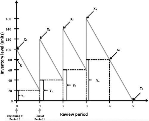
In the example in Figure 1, when a sufficient amount has been accumulated, the excess inventory effectively becomes cycle stock that can be used to satisfy demand. We note, however, that the excess inventory will consume a nontrivial amount of additional storage space. In fact, since the retailer will need enough space to accommodate the maximum amount of inventory carried, the space need is double what it would be if OPS were equal to μ_Z.

3.2. Properties of the inventory

The observations made in Section 3.1 can be generalized for any value of μ_Z and OPS in a deterministic (R, S) setting. We first state four properties of the ending inventory that were observed by conducting multiple simulations with different OPS, mean demand, and CSL values as described in Section 2.1. The standard deviation of demand was set to zero. We later use these properties of the ending inventory to derive the properties of the beginning inventory.

P1. The ending inventory in any time period is an integer multiple of m, the greatest common divisor (GCD) of OPS and the demand over a review period, μ_Z.

P2. After any review period where the ending inventory is 0, there will be a series of review periods in which the ending inventory takes all values from a fixed set of integer multiples of m, such that $Y_n\in \left\{0·m,1·m,2·m,\dots ,\left(\frac{\mathit{OPS}}{m}-1\right)·m\right\}.$

P3. The ending inventory takes these values in an infinitely repeating cycle. The second-to-last value of the cycle is always equal to μ_Z, hence the amount ordered in that review period is 0 and the last value of the cycle is always $0·m,$ given that under deterministic demand the order-up-to level (S) is μ_Z. The values of the ending inventory throughout the cycle are not necessarily monotonically increasing (they are monotonically increasing in our example in Figure 1.

P4. The number of review periods included in any such cycle is $\frac{\mathit{OPS}}{m}.$

The cyclical nature of the ending inventory levels also implies that the amount ordered repeats itself in a predictable, cyclical fashion. With these properties in hand, we can now develop expressions for the three inventory levels that are of interest in understanding how excess inventory affects retail stores. Equation (4)(4) $$\mathit{Average\hspace{0.5em}}\mathit{beginning\hspace{0.5em}}\mathit{inventory}:E\left[X\right]={\mu }_Z+\frac{\mathit{OPS}-m}{2}$$(4) shows the average beginning inventory that is carried for any value of μ_Z and OPS. The equation consists of two parts. The first, μ_Z, is intuitive: In a deterministic setting with an (R, S) policy and no pack size constraints, $S={\mu }_Z$ and store managers can order exactly μ_Z units. The second part, $\frac{\mathit{OPS}-m}{2},$ is the average excess inventory carried due to pack size constraints. Note that if OPS = 1, then m = 1 and the excess inventory term goes to 0. The average cycle stock can be calculated by dividing $S={\mu }_Z$ by two and adding the average excess inventory term. The maximum beginning inventory is shown in Equation (5)(5) $$\mathit{Maximum\hspace{0.5em}}\mathit{beginning\hspace{0.5em}}\mathit{inventory}:X_{\mathit{max}}={\mu }_Z+\mathit{OPS}-m$$(5) . This is the maximum amount of inventory of this SKU that the store will carry. The proofs are shown in Appendix A. (4) $$\mathit{Average\hspace{0.5em}}\mathit{beginning\hspace{0.5em}}\mathit{inventory}:E\left[X\right]={\mu }_Z+\frac{\mathit{OPS}-m}{2}$$(4) (5) $$\mathit{Maximum\hspace{0.5em}}\mathit{beginning\hspace{0.5em}}\mathit{inventory}:X_{\mathit{max}}={\mu }_Z+\mathit{OPS}-m$$(5) where $m=\mathit{GCD}({\mu }_Z,\mathit{OPS})$

4. Effect of OPS on inventory with stochastic demand

We now relax the assumption that demand is deterministic, and instead assume that it is normally distributed, as $Z\sim \mathcal{N}({\mu }_Z,{\sigma }_Z).$ We still assume an infinite-horizon, (R, S) policy. Because the demand is now a random variable, the ending inventory Y_n also becomes a random variable. After each review period, the store manager inspects Y_n and then places an order to return the inventory to at least a level of S, but due to the OPS constraint, is forced to round up to the nearest integer multiple of OPS. Therefore, the beginning inventory X_n is also a random variable. In order to quantify the excess inventory, we need to start by determining the distribution of the beginning inventory, which in turn depends on the distribution of the ending inventory of the previous review period.

This section starts by observing several properties of the beginning and the ending inventory. Based on these properties, we then derive an analytical description of the distribution of the beginning inventory and an expression for the excess inventory. The analytical description is not very practicable, so, following that, we present an approximation and discuss its accuracy.

4.1. Properties of the inventory

We observe the following properties of the ending inventory and the beginning inventory in a stochastic demand setting:

P5. The range of the beginning inventory, $X_n,$ is from $X_{\mathit{min}}=S$ to $X_{\mathit{max}}=S+\mathit{OPS}-1.$

P6. The range of the ending inventory, Y_n, is from Y_min = 0 to $Y_{\mathit{max}}=X_n,$ where X_n is between S and $S+\mathit{OPS}-1$ (from [P5]).

P7. The ending inventory results from subtracting the demand from the beginning inventory, $Y_n=\mathit{max}(0,X_n-Z_n).$ Given that Z_n is normally distributed, $X_n-Z_n$ will also be approximately normally distributed, but the distribution of the ending inventory will be truncated at zero, which is expressed by the max operator.

The proofs for the upper bound stated in [P5], as well as for [P7], are given in Appendix B. The lower bound in [P5] has an intuitive explanation: S is within the range of Y_n, and if Y _n = S, the store manager will not place an order and thus X_n = S. Of course, if $Y_n<S,$ OPS may also be such that the store manager can place an order that returns the inventory level exactly to S. The bounds stated in [P6] flow directly from [P5].

4.2. Analytical description of the distribution of beginning inventory

The beginning inventory $X_{n+1}$ is a function of the ending inventory Y_n and, as stated in [P7], the distribution of Y_n is truncated at 0. We first inspect the distribution of the ending inventory if it were not truncated, and we denote the untruncated ending inventory $Y_n^{(u)}.$ It is given by: $Y_n^{(u)}=X_n-Z_n.$ Note that Z_n may be greater than X_n.

For any particular review period n, X_n will be a constant. We subtract from that a normally distributed Z_n, so $Y_n^{(u)}$ will also be normally distributed, $Y_n^{(u)}\sim \mathcal{N}({\mu }_Y,{\sigma }_Y).$ X_min and X_max are given by [P5] as S and $S+\mathit{OPS}-1$ respectively. We also know that $>99\%$ of all values of Z_n lie within ${\mu }_Z\pm 3·{\sigma }_Z,$ so we can approximate a range of Z_n, with $Z_{\mathit{min}}={\mu }_Z-3·{\sigma }_Z$ and $Z_{\mathit{max}}={\mu }_Z+3·{\sigma }_Z.$ This leads us to: (6) $$Y_{\mathit{min}}^{(u)}\approx S-({\mu }_Z+3·{\sigma }_Z)$$(6) (7) $$Y_{\mathit{max}}^{(u)}\approx S+\mathit{OPS}-1-({\mu }_Z+3·{\sigma }_Z)$$(7)

For tractability, we assume that ${\mu }_Z-3·{\sigma }_Z\ge 0.$ The mean and standard deviation of the untruncated distribution of ending inventory, denoted here as ${\mu }_Y^{(u)}$ and ${\sigma }_Y^{(u)},$ can now be expressed as: (8) $${\mu }_Y^{(u)}=\frac{Y_{\mathit{min}}^{(u)}+Y_{\mathit{max}}^{(u)}}{2}=S-({\mu }_Z+3·{\sigma }_Z)+\frac{\mathit{OPS}-1}{2}$$(8) (9) $${\sigma }_Y^{(u)}=\frac{Y_{\mathit{max}}^{(u)}-{\mu }_Y^{(u)}}{3}=\frac{\mathit{OPS}-1}{6}$$(9)

The truncated distribution of the ending inventory ranges from 0 to $Y_{\mathit{max}}^{(u)}.$ For $Y_n>0,$ it follows the untruncated distribution. However, $P(Y_n=0)=P(Y_n^{(u)}\le 0)=F_{Yn}(Y_n=0),$ which can be calculated using ${\mu }_Y^{(u)}$ and ${\sigma }_Y^{(u)}.$ The discrete probability values for Y_n are found as described in Appendix B.2.

Given the distribution of the ending inventory, and the (deterministic) order quantities that apply to each possible value of the ending inventory, the distribution of the beginning inventory can be constructed. Given that the order quantities do not follow a continuous function, this needs to be done value by value. In what follows, we present an example to illustrate how this is done.

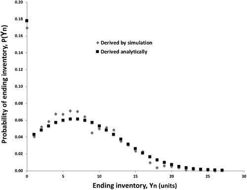
Assume that the demand follows a distribution of $Z_n\sim \mathcal{N}({\mu }_Z=70,{\sigma }_Z=5)$ and that OPS = 10 and S = 72. Table 2 shows the values that the parameters described in this section would take under these assumptions.

Table 2. Parameter values for derivation of beginning inventory distribution.

Parameter	Derived	Value in	Parameter	Derived	Value in
	from	this example		from	this example
Xmin	Property [P5]	72	$Y_{\mathit{min}}^{(u)}$	$X_{\mathit{min}}-Z_{\mathit{max}}$	−13
Xmax	Property [P5]	81	$Y_{\mathit{max}}^{(u)}$	$X_{\mathit{max}}-Z_{\mathit{min}}$	26
Zmin	${\mu }_Z-3·{\sigma }_Z=5$	55	${\mu }_Y^{(u)}$	Eq. 8	6.5
Zmax	${\mu }_Z+3·{\sigma }_Z=5$	85	${\sigma }_Y^{(u)}$	Eq. 9	6.5

Figure 2 shows the probability mass function of the ending inventory for the example parameter values, derived using our proposed method. For comparison, a probability mass function for the same parameter values, but generated by simulation, is also shown. Note the modes at Y _n = 0, which are due to the truncation of the distribution, as well as the overall similarity of the two distributions.

Figure 2. Comparison of probability mass functions of ending inventory.

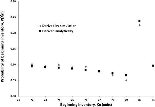
In order to determine the distribution of the beginning inventory, the appropriate order quantity must be added to each possible value of the ending inventory, and then the probabilities are summed up by value of the beginning inventory. To illustrate this, consider the probability of observing a beginning inventory of 80 units. (10) $$P(X_n=80)=P\left(Y_{n-1}+\mathit{OPS}·\lceil \frac{S-Y_{n-1}}{\mathit{OPS}}\rceil =80\right)$$(10) (11) $$=P\left(\frac{Y_{n-1}}{\mathit{OPS}}+\lceil 7.2-\frac{Y_{n-1}}{10}\rceil =\frac{80}{\mathit{OPS}}\right)$$(11) (12) $$=P\left(\frac{Y_{n-1}}{10}+\lceil 7.2-\frac{Y_{n-1}}{10}\rceil =8\right)$$(12)

For Equation (12)(12) $$=P\left(\frac{Y_{n-1}}{10}+\lceil 7.2-\frac{Y_{n-1}}{10}\rceil =8\right)$$(12) to hold, $\frac{Y_{n-1}}{10}$ must be an integer. Since $Y_{n-1}\in [0,26],\frac{Y_{n-1}}{10}=Y_{n-1}^{\prime }\in [0,2.6].$ Therefore, the possible values of $Y_{n-1}^{\prime }$ are 0, 1, and 2. By substituting $Y_{n-1}=\mathit{OPS}·\{0,1,2\}=\{0,10,20\}$ in Equation (12)(12) $$=P\left(\frac{Y_{n-1}}{10}+\lceil 7.2-\frac{Y_{n-1}}{10}\rceil =8\right)$$(12) , we find: (13) $$P(X_n=80)=P(Y_{n-1}=0)+P(Y_{n-1}=10)+P(Y_{n-1}=20)$$(13) (14) $$=0.178+0.053+0.007$$(14) (15) $$=0.238$$(15)

All other P(X_n) are calculated using the same procedure. Figure 3 shows a comparison of the probability mass function for the beginning inventory derived via our proposed method and a probability mass function generated by simulation with the same parameter values. Again, one can appreciate the similarity of the results. The simulation yields an average beginning inventory of 76.8, whereas the distribution derived via the proposed method has a mean of 76.9. One can also see that the mode of the distribution stands out as considerably larger than any other values. This is a general characteristic of the distribution of the beginning inventory; it is a consequence of the truncation of the distribution of the ending inventory at 0.

Figure 3. Comparison of probability mass functions of beginning inventory.

4.3. Approximation of the distribution of the beginning inventory

The derivation of the distribution of the beginning inventory described in Section 4.2 is a multi-step process that does not result in a continuous function. Therefore, the resulting distribution is difficult to use in optimization models, and important measures such as the average beginning inventory are not readily calculated.

As a mathematically more tractable alternative, we propose an approximation of the distribution of the beginning inventory as a uniform distribution ranging from S to $S+\mathit{OPS}-1.$ In typical implementations of (R, S) policies, S is usually set as ${\mu }_Z+T,$ where T is the safety stock. The accuracy of the approximation as a uniform distribution will be further discussed in Section 4.4, but first, we present the expressions for the average beginning inventory and the maximum beginning inventory using this approximation.

The average beginning inventory for any value of μ_Z, T, and OPS is shown in Equation (16)(16) $$\mathit{Average\hspace{0.5em}}\mathit{beginning\hspace{0.5em}}\mathit{inventory}:E\left[X\right]={\mu }_Z+T+\frac{\mathit{OPS}-1}{2}$$(16) . This is in fact the average of the uniform distribution, and $\frac{\mathit{OPS}-1}{2}$ is the average excess inventory that is carried due to the OPS constraint. The average cycle stock can be found by dividing μ_Z by two and adding the safety stock and the expression for the average excess inventory. The maximum beginning inventory is in Equation (17)(17) $$\mathit{Maximum\hspace{0.5em}}\mathit{beginning\hspace{0.5em}}\mathit{inventory}:X_{\mathit{max}}={\mu }_Z+T+\mathit{OPS}-1$$(17) , which is the upper bound of the proposed uniform distribution approximation.

When comparing Equations (16)(16) $$\mathit{Average\hspace{0.5em}}\mathit{beginning\hspace{0.5em}}\mathit{inventory}:E\left[X\right]={\mu }_Z+T+\frac{\mathit{OPS}-1}{2}$$(16) and (17)(17) $$\mathit{Maximum\hspace{0.5em}}\mathit{beginning\hspace{0.5em}}\mathit{inventory}:X_{\mathit{max}}={\mu }_Z+T+\mathit{OPS}-1$$(17) to Equations (4)(4) $$\mathit{Average\hspace{0.5em}}\mathit{beginning\hspace{0.5em}}\mathit{inventory}:E\left[X\right]={\mu }_Z+\frac{\mathit{OPS}-m}{2}$$(4) and (5)(5) $$\mathit{Maximum\hspace{0.5em}}\mathit{beginning\hspace{0.5em}}\mathit{inventory}:X_{\mathit{max}}={\mu }_Z+\mathit{OPS}-m$$(5) in Section 3.2, it can be seen that $\mathit{OPS}-1\ge \mathit{OPS}-m$ since $m\ge 1.$ In other words, compared to the case of deterministic demand, stochastic demand generally increases the average excess inventory due to OPS constraints. This is a consequence of the larger range of ending inventory levels that are experienced when demand is stochastic. (16) $$\mathit{Average\hspace{0.5em}}\mathit{beginning\hspace{0.5em}}\mathit{inventory}:E\left[X\right]={\mu }_Z+T+\frac{\mathit{OPS}-1}{2}$$(16) (17) $$\mathit{Maximum\hspace{0.5em}}\mathit{beginning\hspace{0.5em}}\mathit{inventory}:X_{\mathit{max}}={\mu }_Z+T+\mathit{OPS}-1$$(17)

4.4. Accuracy of the approximation

We now discuss the accuracy of the uniform distribution approximation. By inspecting the probability distributions shown in Figure 3, it becomes clear that the approximation by a uniform distribution will miss certain characteristics of the distribution, for instance, the slight downward trend of the probability values as X_n increases or, perhaps more importantly, the mode. It is important to emphasize that this is an approximation, created for mathematical convenience but at the cost of some level of detail. Nonetheless, the uniform distribution approximation results in an average beginning inventory that is very close to the simulated value; in Section 4.2, where we illustrate the process of analytically deriving the distribution of beginning inventory, the approximated mean is 76.9 and the simulated value is 76.8.

A series of Monte Carlo simulations was run with different values of OPS, mean demand, and standard deviation of demand as described in Section 2.1, and the results were compared to the values calculated with Equation (16)(16) $$\mathit{Average\hspace{0.5em}}\mathit{beginning\hspace{0.5em}}\mathit{inventory}:E\left[X\right]={\mu }_Z+T+\frac{\mathit{OPS}-1}{2}$$(16) . A comparison of simulation results with values calculated using Equation (17)(17) $$\mathit{Maximum\hspace{0.5em}}\mathit{beginning\hspace{0.5em}}\mathit{inventory}:X_{\mathit{max}}={\mu }_Z+T+\mathit{OPS}-1$$(17) was not necessary since Equation (17)(17) $$\mathit{Maximum\hspace{0.5em}}\mathit{beginning\hspace{0.5em}}\mathit{inventory}:X_{\mathit{max}}={\mu }_Z+T+\mathit{OPS}-1$$(17) is exact, as is proven in Appendix B. Overall, the results suggest that Equation (16)(16) $$\mathit{Average\hspace{0.5em}}\mathit{beginning\hspace{0.5em}}\mathit{inventory}:E\left[X\right]={\mu }_Z+T+\frac{\mathit{OPS}-1}{2}$$(16) is a very good approximation. Across the 25,200 simulation runs, the root mean square error (RMSE) for the average beginning inventory is 0.97, and the mean absolute percentage error (MAPE) for the average beginning inventory is 0.6%. As an example, Table 3 shows a comparison of the simulated and calculated average beginning inventory for OPS = 24, five levels of mean demand, and a coefficient of variation of demand of 0.3. The low measures of error confirm that overall, Equation (16)(16) $$\mathit{Average\hspace{0.5em}}\mathit{beginning\hspace{0.5em}}\mathit{inventory}:E\left[X\right]={\mu }_Z+T+\frac{\mathit{OPS}-1}{2}$$(16) is a good approximation of the simulation results.

Table 3. Sample results comparing simulated and calculated results.

Mean	E[X]	E[X]
demand	(simulation)	(Eq. 16(16) $$\mathit{Average\hspace{0.5em}}\mathit{beginning\hspace{0.5em}}\mathit{inventory}:E\left[X\right]={\mu }_Z+T+\frac{\mathit{OPS}-1}{2}$$(16) )
10	26.4	26.5
30	56.3	56.5
60	101.1	101.5
90	146.5	146.5
120	191.7	191.5

Accuracy measures for this subsample only:

RMSE: 0.22; MAPE: 0.31%

5. Effect of OPS constraints on stock-outs

A stock-out (SO) is an event where demand in a review period exceeds beginning inventory (Z_n > X_n), potentially resulting in lost sales. When demand is stochastic, store managers try to minimize stock-outs by holding safety stock T (Silver et al. 2016). The level of safety stock is determined by the desired probability that no stock-out will occur during a review period, i.e., by the cycle service level (CSL): (18) $$\mathit{CSL}=1-P(SO)=1-P(Z_n>X_n)$$(18)

With normally distributed demand and no replenishment lead time, the level of safety stock can be calculated with a safety factor k, i.e., the number of standard deviations above the mean demand for which product is stocked (Silver et al. 2016): (19) $$X_n={\mu }_Z+T={\mu }_Z+{\sigma }_Z·k$$(19)

(R, S) replenishment policies generally assume that the store is able to order up to a level of exactly $S={\mu }_Z+T,$ which implies that the product can be ordered as individual units. In Section 5.1, we explore the effect of OPS constraints on the overall probability of a stock-out. Then, in Section 5.2, we quantify the effect of OPS on the number of units by which the store is short in the case of a stock-out.

5.1. Overall probability of stock-out

If the product can be ordered in individual units, the beginning inventory X_n is always equal to S. Therefore, the probability of a stock-out is calculated as: (20) $$P(SO)=1-F_N\left(\frac{S-{\mu }_Z}{{\sigma }_Z}\right)$$(20)

Here, F_N is the standard normal cumulative distribution function. When there are OPS constraints (i.e., when OPS > 1), it could result in non-negligible amounts of excess inventory carried in stores, which in turn can be used as additional safety stock. As a consequence, the store will be effectively holding inventory corresponding to a higher safety factor $k^{*}$ than originally planned, resulting in a higher cycle service level.

Assume that CSL is the “intended” cycle service level from which S is derived without considering OPS constraints. If, due to the OPS constraint, the beginning inventory exceeds S, the cycle service level actually achieved is CSL*, and CSL*>CSL. With OPS constraints, the beginning inventory X_n is now a random variable. Using the approximation of the distribution of X_n as being uniform between S and $S+\mathit{OPS}-1,$ it can be shown that: (21) $$P{(SO)}^{*}=1-CS{L}^{*}=1-\frac{1}{2·(\mathit{OPS}-1)}{\int }_S^{S+\mathit{OPS}-1}1+\mathit{erf}\left(\frac{x-{\mu }_Z}{{\sigma }_Z·\sqrt{(2)}}\right) dx$$(21)

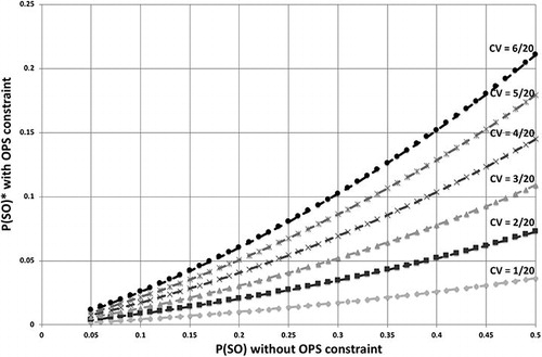
P(SO)* is the stock-out probability that is achieved when the store still uses an order-up-to level that includes the full safety stock required if OPS = 1, but is constrained to order in integer multiples of OPS. The derivation is shown in Appendix C.1. Figure 4 illustrates the relation between P(SO) without OPS constraints (Equation (20)(20) $$P(SO)=1-F_N\left(\frac{S-{\mu }_Z}{{\sigma }_Z}\right)$$(20) ) and P(SO)* with OPS constraints (Equation (21)(21) $$P{(SO)}^{*}=1-CS{L}^{*}=1-\frac{1}{2·(\mathit{OPS}-1)}{\int }_S^{S+\mathit{OPS}-1}1+\mathit{erf}\left(\frac{x-{\mu }_Z}{{\sigma }_Z·\sqrt{(2)}}\right) dx$$(21) ). The illustration assumes normally distributed demand with ${\mu }_Z=20,$ and in the case with OPS constraints, OPS = 12. Each line represents a different coefficient of variation, ranging from 0.05 (1/20) to 0.3 (6/20). In all cases, the probability of a stock-out with the OPS constraint is considerably lower than without; for instance, in the case of a coefficient of variation of 0.3, the drop ranges from −58% to −77%. As can be seen, increasing variability in demand results in a larger P(SO)* and thus a steeper slope.

Figure 4. Probability of stock-out with and without OPS constraints, with varying standard deviation of demand.

Furthermore, it is informative to consider the effect of the pack size itself on the cycle service level. For that purpose, Figure 5 again shows the relation between P(SO) without OPS constraints (Equation (20)(20) $$P(SO)=1-F_N\left(\frac{S-{\mu }_Z}{{\sigma }_Z}\right)$$(20) ) and P(SO)* with OPS constraints (Equation (21)(21) $$P{(SO)}^{*}=1-CS{L}^{*}=1-\frac{1}{2·(\mathit{OPS}-1)}{\int }_S^{S+\mathit{OPS}-1}1+\mathit{erf}\left(\frac{x-{\mu }_Z}{{\sigma }_Z·\sqrt{(2)}}\right) dx$$(21) ), but this time, both the mean demand and the coefficient of variation are kept constant, at ${\mu }_Z=20$ and CV = 0.3. Demand is assumed to be normally distributed, and the OPS is varied from 1 to 35. As expected, for OPS = 1, the line is at a 45 degree angle. As OPS increases, the slope of the line decreases, as larger pack sizes lead to increased excess inventory that in turn acts as a buffer against demand uncertainty, driving down P(SO).

Figure 5. Probability of stock-out with and without OPS constraints, with varying OPS.

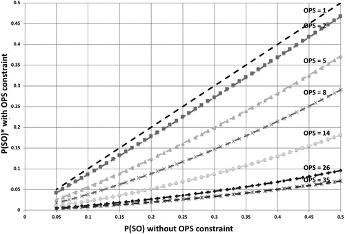
We validated our results in two ways. First, the simulation presented in Section 2.1 was repeated using the empirical demand distribution for a popular product at Deltaco, but with varying OPS. The results were very similar to those shown in Figure 5. Second, the simulation presented in Section 2.1 was extended to include the stock-out probability. For the 25,200 Monte Carlo simulation runs, the root mean square error (RMSE) was $2·{10}^{-4}$ and the mean absolute percentage error (MAPE) was 6.7%. Both measures indicate a close match between the simulation and the analytical results. As an example, Table 4 shows a comparison of the simulated and calculated stock-out probability for the same parameters as were used in Table 3.

Table 4. Comparison of P(SO)* from simulation and analytical method.

Mean	P(SO)*	P(SO)*
Demand	simulation	Eqn. 21
10	0.023	0.020
30	0.076	0.071
60	0.139	0.131
90	0.164	0.170
120	0.203	0.202

Accuracy measures for this subsample only:

RMSE: $5·{10}^{-3};$ MAPE: 7.4 %

5.2. Expected number of units short

If a stock-out occurs, it is important to know how many units the store is short, since each unit short represents a potential lost sale. We denote units short as L. If we assume demand to be normally distributed, the expected number of units short, $E[L],$ can also be derived using the uniform distribution approximation of the beginning inventory. Conceptually, $E[L]$ is equal to $E[\mathit{max}(Z_n-X_n,0)].$ If there are no OPS constraints, and the SKU can be ordered in single-unit increments, the expected number of units short is: (22) $$E\left[L\right]={\sigma }_Z·G_N\left(\frac{S-{\mu }_Z}{{\sigma }_Z}\right)$$(22) $G_N(.)$ is the unit normal loss function. With OPS constraints, when OPS > 1, the expected number of units short can be shown to be: (23) $$E{\left[L\right]}^{*}=\frac{1}{2(\mathit{OPS}-1)}·{\int }_0^{\infty }l·\left[\mathit{erf}\left(\frac{S+l+\mathit{OPS}-1-{\mu }_Z}{\sqrt{2}{\sigma }_Z}\right)-\mathit{erf}\left(\frac{S+l-{\mu }_Z}{\sqrt{2}{\sigma }_Z}\right)\right] dl$$(23)

The derivation can be found in Appendix C.2. Figure 6 shows an example of how $E{[L]}^{*}$ and the cycle service level vary as OPS increases. The figure was generated using a normally distributed demand with ${\mu }_Z=70$ and ${\sigma }_Z=15.$ S was set at 80 units. OPS is shown on the horizontal axis and ranges from 1 to 100. The baseline result includes $E[L]$ and the cycle service level for OPS = 1, as calculated with Equations (22)(22) $$E\left[L\right]={\sigma }_Z·G_N\left(\frac{S-{\mu }_Z}{{\sigma }_Z}\right)$$(22) and (20)(20) $$P(SO)=1-F_N\left(\frac{S-{\mu }_Z}{{\sigma }_Z}\right)$$(20) . For each value of OPS, $E{[L]}^{*}$ and the cycle service level were then calculated using Equations (23)(23) $$E{\left[L\right]}^{*}=\frac{1}{2(\mathit{OPS}-1)}·{\int }_0^{\infty }l·\left[\mathit{erf}\left(\frac{S+l+\mathit{OPS}-1-{\mu }_Z}{\sqrt{2}{\sigma }_Z}\right)-\mathit{erf}\left(\frac{S+l-{\mu }_Z}{\sqrt{2}{\sigma }_Z}\right)\right] dl$$(23) and (21)(21) $$P{(SO)}^{*}=1-CS{L}^{*}=1-\frac{1}{2·(\mathit{OPS}-1)}{\int }_S^{S+\mathit{OPS}-1}1+\mathit{erf}\left(\frac{x-{\mu }_Z}{{\sigma }_Z·\sqrt{(2)}}\right) dx$$(21) . Each data point shows the respective result as a percentage of the baseline result. As one can see, $E{[L]}^{*}$ decreases as OPS increases due to the additional excess inventory that is carried. Both variables show asymptotic behavior, with the largest changes occurring on the lower end of pack sizes.

Figure 6. Expected units short, E[L] (for OPS = 1) and E[L]* (for OPS >1), and cycle service level as a function of OPS.

6. Trade-off between excess space needs and cycle service levels

The discussion so far has shown that increases in OPS have both positive and negative effects. Excess inventory accumulated as a result of order quantity constraints consumes additional storage space, but it also functions as additional safety stock and reduces the average probability of a stock-out. We now discuss the trade-off between the excess space needs and the reduced probability of a stock-out.

Both these variables vary as a function of OPS, but the relationship between them is generally nonlinear. An example is shown in Figure 7, where the percentage change in average beginning inventory and the percentage change in $P{(SO)}^{*}$ are plotted against each other for different values of OPS and different values of planned (“intended”) cycle service level CSL. The figure was generated using normally distributed demand with ${\mu }_Z=70,{\sigma }_Z=15,$ which corresponds to the demand characteristics of a popular item at Deltaco. The vertical axis shows the percentage increase in average beginning inventory with the OPS constraint relative to the average beginning inventory if there were no constraint (i.e., with OPS = 1). The horizontal axis shows the percentage decrease in $P{(SO)}^{*}$ with the OPS constraint relative to P(SO) with OPS = 1. For OPS greater than 1, the average beginning inventory was calculated using Equation (16)(16) $$\mathit{Average\hspace{0.5em}}\mathit{beginning\hspace{0.5em}}\mathit{inventory}:E\left[X\right]={\mu }_Z+T+\frac{\mathit{OPS}-1}{2}$$(16) , and $P{(SO)}^{*}$ was calculated using Equation (21)(21) $$P{(SO)}^{*}=1-CS{L}^{*}=1-\frac{1}{2·(\mathit{OPS}-1)}{\int }_S^{S+\mathit{OPS}-1}1+\mathit{erf}\left(\frac{x-{\mu }_Z}{{\sigma }_Z·\sqrt{(2)}}\right) dx$$(21) . The dotted 45-degree line in the figure indicates the region where the $P{(SO)}^{*}$ would decrease by the same percentage as space requirement increases.

Figure 7. Percentage decrease in stock out probability vs. increase in space requirement for an empirical distribution with different cycle service levels. All percentages are relative to the base case of OPS = 1.

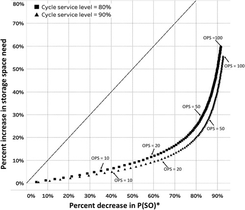
To maintain readability, Figure 7 only shows the cases of planned CSL = 80% and 90%. As can be seen, for a given OPS, the percentage increase in storage space need is lower in the case of planned CSL = 90% than in the case of planned CSL = 80%. This holds in general, for all levels of planned CSL, due to the corresponding change in the order-up-to-level S. Furthermore, the marginal impact of changes in OPS on the average beginning inventory is linear, but the marginal impact on $P{(SO)}^{*}$ is nonlinear. Therefore, for small OPS, an increase in the OPS will lead to a relatively large change in $P{(SO)}^{*},$ whereas the same increase leads to a smaller change in $P{(SO)}^{*}$ when OPS is large.

While the exact locations of the data points will of course be a function of μ_Z and σ_Z, the pattern seen in Figure 7 and the nonlinear effect on $P{(SO)}^{*}$ was consistently observed across many variations of demand characteristics. For an OPS of 20 and a planned CSL of 80%, Figure 7 suggests that Deltaco will in fact achieve a CSL* of 91% for the item due to pack size constraints. Meanwhile, space requirements will be 12% higher than if OPS were 1. If Deltaco were to target a CSL of 90%, the CSL* achieved would in fact be 96% on average, but space requirements would be 11% higher than if OPS were 1. This trade-off could be non-trivial for retailers when considering the multiple items that are stored in the backroom. Thus, across the many items that Deltaco carries in the backroom, the increase in space use is considerable, increasing the risk that Deltaco’s retail stores may become space constrained. However, not all excess inventory translates to higher CSL* and potentially higher revenue: As a LSR chain, many of Deltaco’s products are perishable, so the excess inventory may lead to more product perishing, while also causing higher costs due to the added storage space requirements. This illustrates how retailers need to carefully consider whether the increased costs due to excess inventory and the higher-than-planned CSL* of many products due to pack size constraints, are desirable (“worth it”).

7. Discussion

As was shown in our discussion of the effect of OPS on inventory carried under deterministic and stochastic demand scenarios in Sections 3 and 4, the observed beginning inventory can be close to double the order-up-to level in some cases. The excess inventory that is carried due to OPS constraints has several effects on store costs. First, it will result in additional holding costs and additional in-store logistics costs, since the additional product needs to be handled and stored by employees. Holding costs are readily calculated with the equations presented in this paper, but added in-store logistics costs are more difficult to quantify. Generally speaking, excess inventory across a large number of SKUs can result in very congested backroom areas, which makes it harder for employees to find and store product and to maneuver through the backroom as part of their routine duties. Furthermore, the excess inventory decreases inventory visibility at the time of ordering and increases the risk of perishable goods going to waste.

A large effect on costs and revenue, however, may be indirect and due to the additional storage space that has to be sectioned off in a store. In a single-SKU setting, the overall storage space needs will be driven by the maximum beginning inventory (Equations (5)(5) $$\mathit{Maximum\hspace{0.5em}}\mathit{beginning\hspace{0.5em}}\mathit{inventory}:X_{\mathit{max}}={\mu }_Z+\mathit{OPS}-m$$(5) and (17)(17) $$\mathit{Maximum\hspace{0.5em}}\mathit{beginning\hspace{0.5em}}\mathit{inventory}:X_{\mathit{max}}={\mu }_Z+T+\mathit{OPS}-1$$(17) ). In a multi-SKU setting, it is unlikely that the inventory levels of all SKUs will be at their maximum at the same time, so the sum of the average beginning inventories (Equations (4)(4) $$\mathit{Average\hspace{0.5em}}\mathit{beginning\hspace{0.5em}}\mathit{inventory}:E\left[X\right]={\mu }_Z+\frac{\mathit{OPS}-m}{2}$$(4) and (16)(16) $$\mathit{Average\hspace{0.5em}}\mathit{beginning\hspace{0.5em}}\mathit{inventory}:E\left[X\right]={\mu }_Z+T+\frac{\mathit{OPS}-1}{2}$$(16) ) may be a more appropriate indicator of the overall storage space needs. Nonetheless, across many SKUs, this adds a considerable amount of additional storage space, and this space has to be taken from somewhere. It may result in a larger store footprint, and therefore in higher rent costs. A much more likely scenario, however, is that the additional backroom space will need to be provided at the cost of less customer-facing space.

Additional space needs can arise if the product is stored in inner packs (“intra-packs”) contained within a shipment case. As an example, a shipment case of frozen croissants may contain several smaller cases with the individual croissants. The latter can be taken out of the shipment case for storage in the backroom, but an inner pack is not discarded until the last croissant in it has been removed from the backroom. Thus, the space consumed will be the entire volume of the inner pack until the last consumable unit within it is used and it can be discarded. While there are important reasons to keep SKUs in inner packs (e.g., food safety requirements), this will further decrease the profit per unit volume of storage space that the store can achieve.

Congested backroom areas and space constraints in retail stores can be exacerbated by older store designs that struggle to accommodate growth in customer demand or growth in the variety of SKUs that need to be stored in the backroom. Both issues are becoming more pressing as retailers move toward omni-channel distribution and look to hold more inventory in retail stores to serve online demand, potentially adding SKUs that were previously not held in the store. While in some cases, costly store upgrades and renovations may be inevitable, our results show that some congestion issues may be alleviated by focusing on in-store inventory management and the effect of OPS in driving excess inventory.

Of course, the excess inventory does not only have negative consequences. As we showed, in a setting with stochastic demand, the excess inventory can also be used as additional safety stock to hedge against higher-than-expected demand, thus increasing the cycle service level. As the excess inventory fluctuates across review periods, the achieved cycle service level CSL* will also fluctuate, though it is expected to always be greater than or equal to the planned cycle service level CSL. Store managers can choose to accept this as a benefit of OPS constraints, or they can choose to reduce the amount of safety stock that is carried, which in turn would recover some of the costs incurred due to the excess inventory (i.e., plan for $\mathit{CSL}\prime ,$ where $\mathit{CSL}\prime <\mathit{CSL}$). However, if they do the latter, it is likely that CSL* will occasionally dip below the originally planned CSL due to the fluctuating nature of the excess inventory.

8. Conclusions

In this paper, we investigate the effect of OPS on backroom inventory, space needs, and cycle service levels in retail stores. Store managers are constrained to ordering only in multiples of OPS, which may be different than the optimal order quantity. If store managers calculate the optimal order quantity and then round up to the nearest multiple of OPS, this can result in stores accumulating excess inventory. Our discussion is limited to a single SKU, and we quantify the effect of OPS constraints on inventory levels for the cases of deterministic and stochastic demand. Furthermore, we quantify the link between excess inventory, the expected probability of stock-out, and the expected units short.

Of course, the impact of the excess inventory on holding costs is highly dependent on the value of the goods, and it may well be negligible for cheap commodities. Excess space needs, on the other hand, are likely to be a cost driver, especially when added up across a large number of SKUs and a large number of stores (for instance, Deltaco typically stores several hundred SKUs in the backroom). This is particularly pressing for retail chains that operate in dense urban areas with relatively high rents. Having to provide a larger backroom in retail stores generally entails an opportunity cost resulting from cutting into the revenue generating space of the store.

Our results show that it is important to use inventory policies that incorporate the effect of pack sizes in optimal order quantity recommendations. Commonly used inventory policies ignore the OPS constraint, leading to erroneous inventory projections and potentially sub-optimal order quantities. Moreover, it would be advantageous for retailers to have a universal policy on the level of safety stock to be carried if there is excess inventory due to pack size constraints. These updates need to be reflected in inventory management systems. Failing that, the outcomes are likely to be damaging to the profitability of the retailer: Store managers may either develop their own heuristic methods for determining order quantities, which may involve always rounding up and thus accumulating excess inventory, or they may lose confidence in the inventory management system and disregard its recommendations.

8.1. Managerial implications

The insights discussed in this paper have several managerial implications. First, they demonstrate the value of conducting store-level analyses to understand the trade-off between space needs and store profits. If stores can quantify the mean and standard deviation of demand for SKUs, planners can use data on excess inventory to identify “worst offenders” in the backroom. These are SKUs that require a lot of storage space while yielding a low profit per unit volume of storage space. In an LSR setting, where SKUs stored in the backroom are combined and processed by store personnel to create the end products that are sold to customers, this requires precise data tracking backroom inventories. Alternatively, planners may use a combination of point-of-sale data with ingredient breakdowns and a quantification of product waste levels. At the system level, managers must be aware of the consequences of an “ad-hoc” approach to determining OPS. Our paper demonstrates the importance of conducting thoughtful, rigorous analyses and optimizations to determine the OPS of products. To do so, graphs such as Figure 7 can be used to visualize some of the costs and benefits of changing the OPS. There are obviously trade-offs to be made. A larger OPS reduces handling costs throughout the supply chain (Wen et al. 2012) and increases average cycle service levels, leading to lower penalty costs due to stock-outs. However, the larger the OPS, the more excess inventory is likely to be accumulated in stores, leading to other costs.

In a setting with hundreds or thousands of SKUs being held in one retail store, and as many retail stores within the network, determining an optimal OPS for each SKU becomes a very complex problem. In each store, the storage space needs will be the result of interactions between the many SKUs, and the optimal OPS will vary by SKU and store combination. While this will be the subject of forthcoming research, until further results and optimization tools are available, we recommend that at a minimum, managers use approaches such as those illustrated in this paper to quantify and visualize the impact of different OPS at the store level. This may help determine heuristically whether benefits could be derived from adjusting the OPS of a given SKU, especially across all stores served by a distribution center. Ideally, system-level OPS decisions should also consider the aggregate impact of different OPS in upstream distribution centers in order to perform network-level optimizations (Hassini 2008). Lastly, our results should make managers aware that the benefits and costs of changing the OPS of an item depend on both the magnitude of the change and the starting point (i.e., the original pack size).

8.2. Limitations

There are several limitations associated with this research. First, the approximation for stochastic demand that we derived relies on several assumptions, notably that demand is normally distributed and that the retailer follows an (R,S) inventory system with periodic review and order-up-to-levels. This limits the applicability of this approximation, and we did not consider how it might perform with other inventory systems or demand distributions. Second, all our results are based on the assumption of a lost sales context where there is no back-ordering of inventory. Thus, while the insights derived in this paper can be generalized to many retail settings beyond LSRs, they are not applicable if back-ordered inventory can occur. Third, the setting of our research also gave rise to the assumption that store managers would always round up orders to the nearest integer of OPS, as discussed in Section 2. This assumption may not hold in other retail settings and also depends on company policy, i.e., to what extent the company penalizes store managers for understocking. It would need to be relaxed for retail settings where the holding costs associated with carrying excess inventory exceed the potential costs of lost sales. Fourth, we did not consider the restocking of the sales floor using inventory held in the backroom. This was again based on the LSR context where, typically, no inventory is held in the frontroom and employees retrieve products as needed from the backroom. This assumption does not hold for other store types, such as grocery stores. In such cases, frontroom and backroom inventory should be treated separately and the cost of restocking the frontroom should be included in store-level inventory models. Finally, the discussions in this paper are limited to a single-SKU setting. Considering that the space needs of, and demand for, many SKUs may interact, this will need to be expanded to a multiple-SKU setting in order to be used for comprehensive inventory planning and space allocation models in retail stores.

8.3. Future research directions

This paper represents an analysis of the behavior of inventory in retail stores in the presence of OPS constraints and derives tractable approximations that can be used in optimization models for space allocation. This builds a foundation for multiple directions of future research. First, the approximations presented here can be used as inputs to large-scale optimization models to determine the optimal allocation of space in space constrained stores carrying multiple SKUs that are competing for limited storage space. Given that one of the objectives was to derive approximations that are computationally cheap, they can also be integrated in models for daily inventory planning at the store level. The expressions for inventory behavior presented here can further serve as inputs to optimization models for determining the optimal OPS, at a single-SKU, single-store level, or at the level of a supply chain with multiple SKUs. The development of such models will be pursued in forthcoming research. As briefly discussed in Section 7, future research should also take into account the effect of inner packs used for storage and possibly consider the optimization of the size of the inner pack as well.

There are two further directions of future work that can use this research as a foundation. First, the analyses presented in this paper should be extended to include shelf life considerations, and thus to account for costs and inventory shrinkage due to perishing items. This would be especially valuable in the food service context. Second, the analyses should be generalized to additional demand distributions for stochastic demand and additional inventory replenishment policies, thus relaxing some of the assumptions identified as limitations in Section 8.2. Lastly, in LSR chains, many of the product offerings are prepared in the retail stores, so one sellable item may consist of multiple ingredient SKUs that have to be ordered separately. The inventory management problem thus must account for orderable SKUs that are ingredients to multiple sellable end products, each with its own demand profile. Future research should address ways to incorporate these constraints and complexities in the models developed here.

Acknowledgement

The authors are grateful to Deltaco for their generous support of this research. Deltaco provided input in the formulation of the research question and provided the data that were used for evaluation purposes.

Disclosure statement

No potential conflict of interest was reported by the authors.

Appendix

A. effect of OPS on inventory with deterministic demand

We provide the proof for Equation (4)(4) $$\mathit{Average\hspace{0.5em}}\mathit{beginning\hspace{0.5em}}\mathit{inventory}:E\left[X\right]={\mu }_Z+\frac{\mathit{OPS}-m}{2}$$(4) . To do so, we focus on one cycle as described in [P2]; since this cycle repeats indefinitely, average inventories during that cycle are also equal to long-run average inventories in an infinite-horizon setting. Within this cycle, the cumulative sum of ending inventory will be: (24) $$\sum _{j=0}^{\frac{\mathit{OPS}}{m}-1}j·m$$(24)

After review period n, the store manager places an order for $\lceil \frac{S-Y_n}{\mathit{OPS}}\rceil =\lceil \frac{{\mu }_Z-Y_n}{\mathit{OPS}}\rceil$ items. Therefore, the beginning inventory in period n is the sum of the ending inventory from period n − 1 and the quantity ordered in period n − 1, and the cumulative sum of beginning inventory within the cycle will be: (25) $$\sum _{j=0}^{\frac{\mathit{OPS}}{m}-1}j·m+\mathit{OPS}·\lceil \frac{{\mu }_Z-j·m}{\mathit{OPS}}\rceil$$(25)

To find the average beginning inventory, we divide Equation (25)(25) $$\sum _{j=0}^{\frac{\mathit{OPS}}{m}-1}j·m+\mathit{OPS}·\lceil \frac{{\mu }_Z-j·m}{\mathit{OPS}}\rceil$$(25) by the duration of the cycle, which is $\frac{\mathit{OPS}}{m}$ according to [P4]. This yields: (26) $$\frac{1}{\frac{\mathit{OPS}}{m}}·\sum _{j=0}^{\frac{\mathit{OPS}}{m}-1}j·m+\mathit{OPS}·\lceil \frac{{\mu }_Z-j·m}{\mathit{OPS}}\rceil =\frac{\mathit{OPS}-m}{2}+\left[m·\sum _{j=0}^{\frac{\mathit{OPS}}{m}-1}\lceil \frac{\frac{{\mu }_Z}{m}-j}{\frac{\mathit{OPS}}{m}}\rceil \right]$$(26)

We use the following relation, which is valid for any positive a, b (Graham et al. 1994), to simplify the summation: (27) $$\lceil \frac{a}{b}\rceil +\lceil \frac{a-1}{b}\rceil +\lceil \frac{a-2}{b}\rceil +\cdots +\lceil \frac{a-b+1}{b}\rceil =a$$(27)

Therefore, Equation (26)(26) $$\frac{1}{\frac{\mathit{OPS}}{m}}·\sum _{j=0}^{\frac{\mathit{OPS}}{m}-1}j·m+\mathit{OPS}·\lceil \frac{{\mu }_Z-j·m}{\mathit{OPS}}\rceil =\frac{\mathit{OPS}-m}{2}+\left[m·\sum _{j=0}^{\frac{\mathit{OPS}}{m}-1}\lceil \frac{\frac{{\mu }_Z}{m}-j}{\frac{\mathit{OPS}}{m}}\rceil \right]$$(26) becomes: (28) $$\frac{\mathit{OPS}-m}{2}+m·\frac{{\mu }_Z}{m}={\mu }_Z+\frac{\mathit{OPS}-m}{2}$$(28)

To find Equation (5)(5) $$\mathit{Maximum\hspace{0.5em}}\mathit{beginning\hspace{0.5em}}\mathit{inventory}:X_{\mathit{max}}={\mu }_Z+\mathit{OPS}-m$$(5) , we start with property [P4], which states that the maximum ending inventory is $\left(\frac{\mathit{OPS}}{m}-1\right)·m=\mathit{OPS}-m.$ That value is attained at the end of a review period, so it represents what is left over after μ_Z has been consumed. Therefore, the corresponding review period must have started with an inventory level of ${\mu }_Z+\mathit{OPS}-m.$

B. effect of OPS on inventory with stochastic demand

B.1 upper bound of the range of the beginning inventory

We need to prove that $X_n\le S+\mathit{OPS}-1.$ We will prove this by contradiction, so we begin by assuming $X_n>S+\mathit{OPS}-1.$ This implies that $X_n\ge S+\mathit{OPS}.$ The left-hand side of this inequality can be expanded as follows: $$X_n=Y_{n-1}+D_n=Y_{n-1}+\mathit{OPS}·\{\begin{array}{cc}\lceil \frac{S-Y_{n-1}}{\mathit{OPS}}\rceil \hfill & \text{if\hspace{0.5em}}{Y}_{n-1}<S\hfill \\ 0\hfill & \mathit{otherwise}\hfill \end{array}$$

This produces two cases that must both be $\ge S+\mathit{OPS}.$ We inspect these cases separately. First, if $Y_{n-1}<S$: $$\begin{array}{c}{Y}_{n-1}+\mathit{OPS}·\lceil \frac{S-Y_{n-1}}{\mathit{OPS}}\rceil \ge S+\mathit{OPS}\\ \lceil \frac{S-Y_{n-1}}{\mathit{OPS}}\rceil \ge \frac{S-Y_{n-1}}{\mathit{OPS}}+1\end{array}$$

Since the last statement is not true for any $Y_{n-1}\ge 0,$ we have proven by contradiction that $X_n\le S+\mathit{OPS}-1$ if $Y_{n-1}<S.$ Next, we inspect the case where $Y_{n-1}\ge S:$ $$\begin{array}{c}{Y}_{n-1}+0\ge S+\mathit{OPS}\\ X_{n-1}-Z_{n-1}\ge S+\mathit{OPS}\\ Z_{n-1}\le X_{n-1}-(S+\mathit{OPS})\end{array}$$

The last statement is not possible because $Z_{n-1}\ge 0.$ Therefore, we have proven that X_n, the beginning inventory during any review period, is $\le S+\mathit{OPS}-1.$

B.2 distribution of the ending inventory

Property [P7] states that the ending inventory is approximately normally distributed, but that it is truncated at 0. To understand the approximate normal distribution, we begin with the definition of the ending inventory: $$\begin{array}{c}{Y}_n=X_n-Z_n\\ =Y_{n-1}+\mathit{OPS}·\lceil \frac{S-Y_{n-1}}{\mathit{OPS}}\rceil -Z_n\end{array}$$

To simplify this expression, a continuity correction factor can be used (Devore 2011): $$\lceil \frac{S-Y_{n-1}}{\mathit{OPS}}\rceil \approx \frac{S-Y_{n-1}}{\mathit{OPS}}+\frac{1}{2}$$

Therefore, the expression becomes: $$\begin{array}{c}{Y}_n\approx Y_{n-1}+\mathit{OPS}·\left(\frac{S-Y_{n-1}}{\mathit{OPS}}+\frac{1}{2}\right)-Z_n\\ \approx S+\frac{\mathit{OPS}}{2}-Z_n\end{array}$$

The only remaining random variable in this expression is Z_n, which is normally distributed. S and OPS are constants, so the distribution of Y_n is a shifted normal distribution. This distribution is then truncated at 0.

In order to generate the discrete probability values, the continuous probability density function of Z_n needs to be discretized, which can again be achieved using a continuity correction factor (Devore 2011). Furthermore, as noted in Section 4.2, we assume for tractability purposes that ${\mu }_Z-3·{\sigma }_Z\le Z_n\le {\mu }_Z+3·{\sigma }_Z.$ Therefore, in light of the discretization and this assumption, a normalization may need to be applied to the discrete probability values.

C. Effect of OPS constraints on stock-outs

C.1 Overall probability of stock-out

In this section, we derive Equation (21)(21) $$P{(SO)}^{*}=1-CS{L}^{*}=1-\frac{1}{2·(\mathit{OPS}-1)}{\int }_S^{S+\mathit{OPS}-1}1+\mathit{erf}\left(\frac{x-{\mu }_Z}{{\sigma }_Z·\sqrt{(2)}}\right) dx$$(21) by using the uniform distribution approximation for the beginning inventory. We start by expanding the expression for the probability of a stock-out: $$\begin{array}{c}P(SO)=P(Z_n>X_n)\\ =1-P(X_n\ge Z_n)\\ =1-\int {\int }_{x\ge z}{f}_X(x)f_Z(z)dzdx\\ =1-{\int }_{-\infty }^{\infty }{\int }_{-\infty }^x{f}_X(x)f_Z(z) dz dx\\ =1-{\int }_{-\infty }^{\infty }{f}_X(x)F_Z(x) dx\end{array}$$

We approximate $f_X(x)$ as a uniform distribution with the following probability density function: $$f_X(x)=\{\begin{array}{cc}\frac{1}{1-\mathit{OPS}}\hfill & x\in \left[S,S+\mathit{OPS}-1\right]\hfill \\ 0\hfill & \mathit{otherwise}\hfill \end{array}$$

Additionally, we denote by $F^{(N)}(x)$ the cumulative distribution function of a normally distributed random variable. Substituting the respective expressions yields: $$\begin{array}{c}P(SO)=1-{\int }_S^{S+\mathit{OPS}-1}\frac{1}{\mathit{OPS}-1}·F_Z^{(N)}(x) dx\\ =1-{\int }_S^{S+\mathit{OPS}-1}\frac{1}{\mathit{OPS}-1}·\frac{1}{2}\left(1+\mathit{erf}\left(\frac{x-{\mu }_Z}{{\sigma }_Z·\sqrt{2}}\right)\right)dx\\ =1-\frac{1}{2·(\mathit{OPS}-1)}{\int }_S^{S+\mathit{OPS}-1}\left(1+\mathit{erf}\left(\frac{x-{\mu }_Z}{{\sigma }_Z·\sqrt{2}}\right)\right)dx\end{array}$$

The last line is the expression for $P{(SO)}^{*}$ when OPS > 1, as shown in Equation (21)(21) $$P{(SO)}^{*}=1-CS{L}^{*}=1-\frac{1}{2·(\mathit{OPS}-1)}{\int }_S^{S+\mathit{OPS}-1}1+\mathit{erf}\left(\frac{x-{\mu }_Z}{{\sigma }_Z·\sqrt{(2)}}\right) dx$$(21) .

C.2 Expected number of units short

This section presents the derivation of Equation (23)(23) $$E{\left[L\right]}^{*}=\frac{1}{2(\mathit{OPS}-1)}·{\int }_0^{\infty }l·\left[\mathit{erf}\left(\frac{S+l+\mathit{OPS}-1-{\mu }_Z}{\sqrt{2}{\sigma }_Z}\right)-\mathit{erf}\left(\frac{S+l-{\mu }_Z}{\sqrt{2}{\sigma }_Z}\right)\right] dl$$(23) , again by using the uniform distribution approximation for the beginning inventory. Since the number of units short is given by the difference between demand and inventory, and is bounded by 0, we are interested in $E[L]=E[\mathit{max}(Z-X,0)].$ We make use of convolution theory, which states that for two continuous random variables A and B, the probability density function of their sum $C=A+B$ is equal to: $$f_C(c)={\int }_{-\infty }^{\infty }{f}_A(a)f_B(w-a) da$$

First, we derive the general expression for the (unbounded) probability density function of L. L is equal to $Z+(-X),$ and Z and X are both continuous random variables. Following the relation above, the probability density function of L is: $$f_L(l)={\int }_{-\infty }^{\infty }{f}_Z(z)f_{(-X)}(l-z)dz={\int }_{-\infty }^{\infty }{f}_Z(z)f_X(z-l) z.$$

We assume that the probability density function of X, and therefore of Z – L, is a uniform distribution with bounds S and $S+\mathit{OPS}-1.$ Therefore, z is only non-zero on an interval with the following bounds: $$\begin{array}{c}S\le z-l\le S+\mathit{OPS}-1\\ S+l\le z\le S+l+\mathit{OPS}-1\end{array}$$

The probability density function $f_X(x)$ is known (see Appendix C.1). Substituting the bounds and the expression for the probability density function yields: $$\begin{array}{c}{f}_L(l)={\int }_{S+l}^{S+l+\mathit{OPS}-1}{f}_Z(z)\frac{1}{\mathit{OPS}-1} dz\\ =\frac{1}{\mathit{OPS}-1}·{\int }_{S+l}^{S+l+\mathit{OPS}-1}{f}_Z(z)dz\\ =\frac{1}{\mathit{OPS}-1}·\left[F_Z(S+l+\left(\mathit{OPS}-1\right)-F_Z(S)\right]\end{array}$$

Recall that $Z\sim \mathcal{N}({\mu }_Z,{\sigma }_Z),$ so the expression for the cumulative distribution function of Z is known: $$\begin{array}{c}{f}_L(l)=\frac{1}{\mathit{OPS}-1}·\left[\frac{1}{2}\left(1+\mathit{erf}\left(\frac{S+l+\mathit{OPS}-1-{\mu }_Z}{\sqrt{2}{\sigma }_Z}\right)\right)-\frac{1}{2}\left(1+\mathit{erf}\left(\frac{S+l-{\mu }_Z}{\sqrt{2}{\sigma }_Z}\right)\right)\right]\\ =\frac{1}{2\left(\mathit{OPS}-1\right)}·\left[\mathit{erf}\left(\frac{S+l+\mathit{OPS}-1-{\mu }_Z}{\sqrt{2}{\sigma }_Z}\right)-\mathit{erf}\left(\frac{S+l-{\mu }_Z}{\sqrt{2}{\sigma }_Z}\right)\right]\end{array}$$

This is the general expression for $f_L(l).$ The expected number of units short for a given OPS can be found by integrating this function from 0 to $\infty :$ $$\begin{array}{c}E\left[L\right]=E[\mathit{max}(L,0)]\\ ={\int }_0^{\infty }l·f_L(l) dl\\ ={\int }_0^{\infty }l·\frac{1}{2·(\mathit{OPS}-1)}·\left[\mathit{erf}\left(\frac{S+l+\mathit{OPS}-1-{\mu }_Z}{\sqrt{2}{\sigma }_Z}\right)-\mathit{erf}\left(\frac{S+l-{\mu }_Z}{\sqrt{2}{\sigma }_Z}\right)\right] dl\\ =\frac{1}{2(\mathit{OPS}-1)}·{\int }_0^{\infty }l·\left[\mathit{erf}\left(\frac{S+l+\mathit{OPS}-1-{\mu }_Z}{\sqrt{2}{\sigma }_Z}\right)-\mathit{erf}\left(\frac{S+l-{\mu }_Z}{\sqrt{2}{\sigma }_Z}\right)\right] dl\end{array}$$

The last line is the expression for $E{[L]}^{*}$ when OPS > 1, as shown in Equation (23)(23) $$E{\left[L\right]}^{*}=\frac{1}{2(\mathit{OPS}-1)}·{\int }_0^{\infty }l·\left[\mathit{erf}\left(\frac{S+l+\mathit{OPS}-1-{\mu }_Z}{\sqrt{2}{\sigma }_Z}\right)-\mathit{erf}\left(\frac{S+l-{\mu }_Z}{\sqrt{2}{\sigma }_Z}\right)\right] dl$$(23) .

References

- Agrawal N, Smith SA. 2019. Optimal inventory management using retail prepacks. Eur J Oper Res. 274(2):531–544.
- Bischak DP, Robb DJ, Silver EA, Blackburn JD. 2014. Analysis and management of periodic review, order-up-to level inventory systems with order crossover. Prod Oper Manage. 23(5):762–772.
- Broekmeulen RA, Sternbeck MG, van Donselaar KH, Kuhn H. 2017. Decision support for selecting the optimal product unpacking location in a retail supply chain. Eur J Oper Res. 259(1):84–99.
- Cachon GP. 2001. Exact evaluation of batch-ordering inventory policies in two-echelon supply chains with periodic review. Oper Res. 49(1):79–98.
- Caplice C, Das L. 2017. How back-of-mind backrooms rob retailers of profits. CSCMP’s Supply Chain Quarterly, 42–45.
- Chakravarty A. 1986. Quantity discounted inventory replenishments with limited storage space. INFOR: Inf Syst Oper Res. 24(1):12–25.
- Chao X, Zhou SX. 2009. Optimal policy for a multiechelon inventory system with batch ordering and fixed replenishment intervals. Oper Res. 57(2):377–390.
- Chen F. 2000. Optimal policies for multi-echelon inventory problems with batch ordering. Oper Res. 48(3):376–389.
- Curşeu A, van Woensel T, Fransoo J, van Donselaar K, Broekmeulen R. 2009. Modelling handling operations in grocery retail stores: an empirical analysis. J Oper Res Soc. 60(2):200–214.
- Devore JL. 2011. Probability and statistics for engineering and the sciences. Boston, MA: Cengage learning.
- Disney SM, Gaalman GJ, Hedenstierna CPT, Hosoda T. 2015. Fill rate in a periodic review order-up-to policy under auto-correlated normally distributed, possibly negative, demand. Int J Prod Econ. 170:501–512.
- Eroglu C, Williams BD, Waller MA. 2013. The backroom effect in retail operations. Prod Oper Manage. 22(4):915–923.
- Graham RL, Knuth DE, Patashnik O. 1994. Concrete math. A foundation for computer science. Reading, MA: Addison-Wesley.
- Hadley G, Whitin TM. 1963. Analysis of inventory systems. Englewood Cliffs, NJ: Prentice-Hall.
- Hassini E. 2008. Supply chain optimization: current practices and overview of emerging research opportunities. INFOR: Inf Syst Oper Res. 46(2):93–96.
- Huang Y-D, Wee H-M, Praharsi Y, Lo CC. 2019. An integrated vendor–buyer replenishment policy for deteriorating items with fuzzy environment and resource constraint. INFOR: Inf Syst Oper Res. 57(4):667–691.
- Hubner A, Holzapfel A, Kuhn H. 2016. Distribution systems in omni-channel retailing. Bus Res. 9(2):255–296.
- Huh WT, Janakiraman G. 2012. On optimal policies for inventory systems with batch ordering. Oper Res. 60(4):797–802.
- Kiesmüller GP, De Kok A, Dabia S. 2011. Single item inventory control under periodic review and a minimum order quantity. Int J Prod Econ. 133(1):280–285.
- Larsen C, Kiesmüller GP. 2007. Developing a closed-form cost expression for an (r, s, nq) policy where the demand process is compound generalized erlang. Oper Res Lett. 35(5):567–572.
- Li X, Sridharan V. 2008. Characterizing order processes of using (r,nq) inventory policies in supply chains. Omega. 36(6):1096–1104. (A. Special Issue Dedicated to the 2008 Beijing Olympic Games)
- Mou S, Robb DJ, DeHoratius N. 2018. Retail store operations: Literature review and research directions. Eur J Oper Res. 265(2):399–422.
- Noblesse AM, Boute RN, Lambrecht MR, Houdt BV. 2014. Characterizing order processes of continuous review (s,s) and (r,nq) policies. Eur J Oper Res. 236(2):534–547.
- Ozgun T, Taube F, Minner S. 2018. Data-driven retail inventory management with backroom effect. Or Spectr. 40:945–968.
- Pires M, Camanho A, Amorim P. 2020. Solving the grocery backroom sizing problem. Int J Prod Res. 58(18):5707–5720..
- Ramakrishna KS, Sharafali M, Lim YF. 2015. A two-item two-warehouse periodic review inventory model with transshipment. Ann Oper Res. 233(1):365–381.
- Roy S, Bhunia AK, Mukhopadhyay S. 2005. A genetic algorithmic approach on a deterministic inventory model for deteriorating items with shortages. INFOR: Inf Syst Oper Res. 43(3):271–282.
- Shang KH, Zhou SX. 2010. Optimal and heuristic echelon (r, nq, t) policies in serial inventory systems with fixed costs. Oper Res. 58(2):414–427.
- Silver EA. 2008. Inventory management: an overview, Canadian publications, practical applications and suggestions for future research. INFOR: Inf Syst Oper Res. 46(1):15–27.
- Silver EA, Bischak DP. 2011. The exact fill rate in a periodic review base stock system under normally distributed demand. Omega. 39(3):346–349.
- Silver EA, Pyke DF, Thomas DJ. 2016. Inventory and production management in supply chains, 4th Ed. Boca Raton, FL: CRC Press.
- Sinha D, Matta KF. 1991. Multiechelon (r, s) inventory model. Decis Sci. 22(3):484–499.
- Sternbeck MG, Kuhn H. 2014. An integrative approach to determine store delivery patterns in grocery retailing. Transp Res Part E: Logist Transp Rev. 70:205–224.
- Tarim SA, Smith BM. 2008. Constraint programming for computing non-stationary (r, s) inventory policies. Eur J Oper Res. 189(3):1004–1021.
- Teunter RH, Syntetos AA, Babai MZ. 2010. Determining order-up-to levels under periodic review for compound binomial (intermittent) demand. Eur J Oper Res. 203(3):619–624.
- Van Donselaar KH, Gaur V, Van Woensel T, Broekmeulen RA, Fransoo JC. 2010. Ordering behavior in retail stores and implications for automated replenishment. Manage Sci. 56(5):766–784.
- Van Donselaar KH, Gaur V, Woensel T, van Broekmeulen R, Fransoo JC. 2006. An empirical study of ordering behavior of retail stores. Working paper. Eindhoven University of Technology.
- Van Horenbeek A, Buré J, Cattrysse D, Pintelon L, Vansteenwegen P. 2013. Joint maintenance and inventory optimization systems: A review. Int J Prod Econ. 143(2):499–508.
- Van Houtum G-J, Scheller-Wolf A, Yi J. 2007. Optimal control of serial inventory systems with fixed replenishment intervals. Oper Res. 55(4):674–687.
- Van Zelst S, Van Donselaar K, Van Woensel T, Broekmeulen R, Fransoo J. 2009. Logistics drivers for shelf stacking in grocery retail stores: Potential for efficiency improvement. Int J Prod Econ. 121(2):620–632.
- Veinott AF. 1965. The optimal inventory policy for batch ordering. Oper Res. 13(3):424–432.
- Wagner HM. 2002. And then there were none. Oper Res. 50(1):217–226.
- Waller MA, Heintz Tangari A, Williams BD. 2008. Case pack quantity’s effect on retail market share: an examination of the backroom logistics effect and the store-level fill rate effect. Int J Phys Disturb Logist Manage. 38(6):436–451.
- Wen N, Graves SC, Ren ZJ. 2012. Ship-pack optimization in a two-echelon distribution system. Eur J Oper Res. 220(3):777–785.
- Wensing T, Sternbeck MG, Kuhn H. 2018. Optimizing case-pack sizes in the bricks-and-mortar retail trade. Or Spectr. 40(4):913–944.
- Zheng Y-S, Chen F. 1992. Inventory policies with quantized ordering. Naval Res Logist. 39(3):285–305.