Cloud model-based best-worst method for group decision making under uncertainty

Abstract

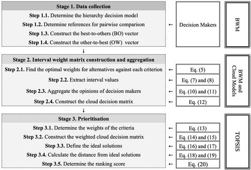
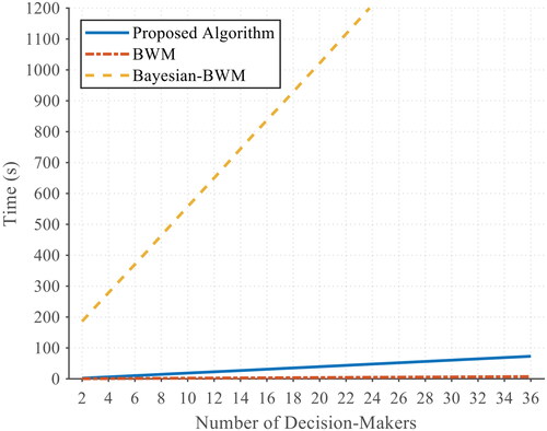
This study aims to enhance computational and analytical aspects of multi-criteria group decision-making (MCGDM) under uncertainty. For this, we use the best-worst method (BWM) and cloud models to develop a more reliable MCGDM algorithm including three stages: first, collecting data through the BWM reference pairwise comparison; second, extracting interval-weights using the BWM bi-level optimisation models and aggregating different opinions via cloud models; and third, using the technique for order of preference by similarity to ideal solution (TOPSIS) to prioritise alternatives. We have also investigated the effectiveness of the proposed approach in a real-life problem of online learning platform selection within the context of the COVID-19 pandemic lockdown. The experiment results demonstrate the superiority of the proposed method over the Bayesian BWM in terms of computational time by 96%. Moreover, the proposed approach outperforms BWM and Bayesian BWM techniques by 33% and 25%, respectively, in terms of conformity to the decision-makers’ intuitive judgments. Our findings also bring important practical implications. Application of the proposed method led to robustness against the number of decision-makers and significantly increased time efficiency in group decision-making. Besides, the computations with the lower inconsistency enhanced the effectiveness of prioritisation in group decision-making.

Keywords:

• Multiple criteria group decision-making
• uncertainty
• cloud models
• interval weights

1. Introduction

Individuals, groups/teams and organisations gather various information to facilitate understanding different situations and forming judgments to make decisions about them (Saaty 2008a). Managing complex conditions entails considering multiple perspectives, and decision-making becomes challenging in such settings (Khorshidi and Aickelin 2021). To address these challenges, several Multi Criteria Decision Making (MCDM) methods have been developed. MCDM is characterised as a sub-discipline of Operations Research (OR) and an important area in the decision-making theory (Rezaei 2015).

Solving a typical MCDM problem usually requires developing a decision matrix, calculating importance weights of criteria and prioritising alternatives. There is a vast array of approaches for weighting criteria, including – but not limited to – the Analytic Hierarchy Process (AHP) (Saaty 1977), Analytic Network Process (ANP) (Saaty and Vargas 2006), Best Worst Method (BWM) (Rezaei 2015), Swing (Mustajoki et al. 2005), and Simple Multi-Attribute Rating Technique (SMART) (Edwards 1977). Forming the decision matrix involves accurate yet straightforward data collection. While data can be retrieved via direct measurement in the case of tangible criteria, it cannot be measured directly for intangible ones (Saaty 2008a). Pairwise comparisons and their relative scales of measurement are well-known solutions for measuring the latter type of data (Saaty 2008b).

AHP, as one of the most prominent pairwise comparison-based methods, entails developing a set of pairwise comparison matrices – organised in a decision hierarchy – which facilitates weighting the compared elements. By defining $a_{\mathit{\text{ij}}}$ as a secondary comparison, if neither i nor j are the most or the least important elements, and $a_{\mathit{\text{rq}}}$ as a reference comparison, if r is the most important and/or q is the least important element, it is argued that secondary comparisons are more complicated and less accurate (Rezaei 2015). Rezaei proposed Best Worst Method (BWM) to derive weights only via reference comparisons, which may lead to easier data collection and more accurate results (Mi et al. 2019), particularly in large problems such as MCGDM.

Decisions made by groups lead to more complete knowledge, a higher level of solution acceptance, as well as more diverse points of view, approaches and alternatives. However, the foremost issue in group decision-making is how to aggregate individual opinions into a single representative opinion. There are two main approaches to do so (Forman and Peniwati 1998). One approach is Aggregation of Individual Judgments (AIJ) (Blagojevic et al. 2016), which aims to aggregate different decision-makers’ pairwise comparisons to achieve a single pairwise comparison and then solve the MCDM problem as a single decision-making problem. The other one, Aggregation of Individual Priorities (AIP) (Abel et al. 2015), is to aggregate the final results (weights) calculated for each decision-maker. Nevertheless, the main basis for aggregation in the mentioned approaches is the average, which causes the following drawback: (i) sensitivity of averages to outliers, which can significantly influence the final results; and (ii) lack of focus on the dispersion effect (Mohammadi and Rezaei 2020). Therefore, developing a more viable aggregation method is necessary.

Besides the aggregation challenge, uncertainty, that may be caused by the lack of knowledge, nature of human thinking or many other possible sources, is another challenge (Durbach and Stewart 2012). The uncertainty sources generally can be classified as (i) inter-expert uncertainty, which refers to the variation of opinions amongst different decision-makers; and (ii) intra-expert uncertainty, that comes from the variation of the opinion of a decision-maker in different situations (Khorshidi and Aickelin 2021).

The most popular remedy for the uncertainty issue is computation with words, which is facilitated by application of linguistic variables (Zadeh 1975). In linguistic variable based techniques, words are usually encoded into numbers using triangular fuzzy numbers (F. Wang 2021), Pythagorean fuzzy environment (Yu et al. 2019), generalised trapezoidal fuzzy numbers (Khorshidi et al. 2016), type-2 fuzzy sets (Meni̇z 2021), hesitant fuzzy sets (Z. Zhang et al. 2021), or cloud models (Y. Liu et al. 2020). However, the primary limitation of these techniques is provision of decision-makers with a limited range of linguistic terms for expressing their opinions (Khorshidi and Aickelin 2021).

Therefore, much attention has been attracted to providing more flexibility for opinion expression through interval values (Wagner et al. 2015) and interval-valued hesitant fuzzy sets (J. Wang et al. 2014). These approaches also have limitations since respondents tend to change their answers when they are queried repeatedly (Havens et al. 2017). In addition, human judgment is always prone to a range of noticeable biases, such as confirmation bias, anchoring bias, and availability bias (Haddad et al. 2020; Rezaei 2021), which can be regarded as examples of intra-expert uncertainty. Moreover, determination of interval values is based on decision-makers’ self-declaration, the validity of which would be questionable due to cognitive biases (Rabiee et al. 2021). Another limitation is that distribution of respondents’ ratings within intervals is simply assumed to be uniform by many scholars (Bode and Wagner 2015).

In the context of addressing challenges in group decision-making, achieving dynamic consensus and consensus efficiency is important for ensuring that all decision-makers’ perspectives and concerns are considered, leading to better-informed and more widely accepted decisions. Dynamic consensus describes the evolution of agreement among group members over time, while consensus efficiency measures the group’s ability to reach consensus effectively. Recent studies have focused on examining the advantages and limitations of dynamic consensus models in managing parameter variability and changing environments, as well as developing more efficient consensus-reaching processes (Pérez et al. 2018; H. Zhang et al. 2019). The TODIM (an acronym in Portuguese for Interactive Multi-criteria Decision Making) method has been proposed as an approach to integrate these concepts, taking into account decision-makers’ preferences and the importance of each criterion in the decision-making process. Additionally, an extended TODIM method has been presented that employs interval type-2 fuzzy sets and prospect theory to solve complex and uncertain multiple criteria group decision-making problems while considering both dynamic consensus and consensus efficiency (Qin et al. 2017).

Given the difficulties outlined, the aim of this study is to devise a method for Multi Criteria Group Decision Making that can tackle the challenges identified. These challenges are summarised in the first two columns of Table 1. We utilise cloud models to resolve the aggregation-related shortcomings, sensitivity to outliers and dispersion effect ignorance occurring in group decision-making. We also address the uncertainty issue of response alteration over queries by performing only reference comparisons, which facilitates data collection through a less number of questions.

Table 1. Causes, effects and solutions for the challenges in MCGDM approaches.

Cause	Effect	Solution	Stage/Step
Group decision-making	Sensitivity of averages to outliers	Using cloud models	Sections 3.2.3 and 3.2.4
	Lack of focus on the dispersion effect
Uncertainty	Response alteration during repetition	A more straightforward data collection process with fewer questions	Section 3.1
	Examples of intra-expert uncertainty	Interval values	Section 3.2
	Self-declaration of interval values	Extracting interval weights by solving optimisation models	Sections 3.2.1 and 3.2.2
	Uniform distribution assumption	Using the Gaussian membership function to capture uncertainty in intervals	Section 3.2.3

The intra-expert uncertainty problem can be alleviated via the application of interval values. However, regarding its cognitive biases, self-declaration appears not to be an error-free method for such data collection. As a result, the present study obtains interval values indirectly, using Rezaei’s (Rezaei 2016) BWM mathematical models. In other words, when there are inconsistencies in pairwise comparisons, which can be originated from decision-makers’ uncertainty, the upper and lower bounds of interval values will be calculated by solving the relevant bi-level optimisation models.

The MCGDM algorithm proposed in this research also focuses on relaxation of the uniform distribution assumption for respondents’ ratings by applying the Gaussian membership function to capture uncertainty in intervals. For this, we utilise cloud models to aggregate interval-valued data. Also, the bi-level optimisation model introduced by Khorshidi and Aickelin (2021), is used through the aggregation process to derive weights of criteria.

2. Preliminaries

2.1. Best worst method

The Best Worst Method (BWM), proposed by Rezaei (Rezaei 2015), is an MCDM approach on the basis of pairwise comparisons, which has attracted much attention due to its advantages over other pairwise comparison-based techniques such as AHP (Mi et al. 2019). In BWM, weights of criteria are derived only by means of reference comparisons, that is, 2n-3 pairwise comparisons versus the larger number of comparisons, n(n-1)/2, required in AHP – where n denotes the number of criteria. Therefore, BWM is more appropriate than AHP for large MCGDM problems. Also, data gathering is much easier in BWM because only integer numbers 1, 2, …, 9 are needed, in comparison to the more complex scale of 1/9 to 9 in AHP. Furthermore, the omitted secondary comparisons in BWM leads to protecting consistency of pairwise comparisons in the approach. It should be added that BWM has been widely utilised in real-life problems, including supply chain management (Rezaei et al. 2016), manufacturing (Ren 2018), energy (van de Kaa et al. 2019), and healthcare (Mou et al. 2016). There have been several studies, such as (Raj and Srivastava, 2018) and (Chen and Ming 2020), that use BWM in an integrated algorithm to solve problems. The following are the BWM steps:

Step 1. Selecting criteria; Step 2. Selecting the best (most desirable) and the worst (least desirable) criteria; Step 3. Comparing the best criterion with all criteria; Step 4. Comparing all criteria with the worst criterion; Step 5. Solving the following optimisation model to obtain optimal weights for criteria. (1) $$\begin{array}{c}\mathit{\text{min}}\underset{j}{\mathrm{\text{max}}}\left\{\left|w_B/w_j-a_{\mathit{\text{Bj}}}\right|,\left|w_j/w_W-a_{\mathit{\text{jW}}}\right|\right\}\\ \mathrm{s}.\mathrm{t}.\sum _{j=1}^n{w}_j=1,w_j\ge 0,\forall j=1,\dots ,n\end{array}$$(1)

When the number of criteria is greater than three, the model may result in multi-optimality because the pairwise comparison is not always fully consistent. However, there exist two solutions for the problem (Rezaei 2016): (i) transforming the min-max nonlinear problem into a linear problem; or (ii) calculating interval weights and conducting an interval analysis. In this paper, we calculate the interval weights using BWM and use them to construct the cloud decision matrix for a group decision-making problem.

2.2. Interval-valued data

After (Billard and Diday 2003) introduced symbolic data, application of interval-valued data attracted much attention amongst scholars and data analysts. This type of data can represent natural variability of a phenomenon and the uncertainty existing in error measurement (de Carvalho et al. 2021). Often, employing interval-valued data is much more suitable than using single crisp values in everyday life, e.g. in the case of imprecise or tolerance-needing measurement; multiple-time data collection within a single unitary period, like time series of air pollution or temperature; and when original data summarisation into single crisp data result in a huge information loss. Thus, it has been utilised in several applications, such as prediction (de Carvalho et al. 2021), classification (Maadi et al. 2020), and decision analysis (Fernández et al. 2022). In this paper, we use it to capture decision-makers’ uncertainty.

2.3. Cloud models

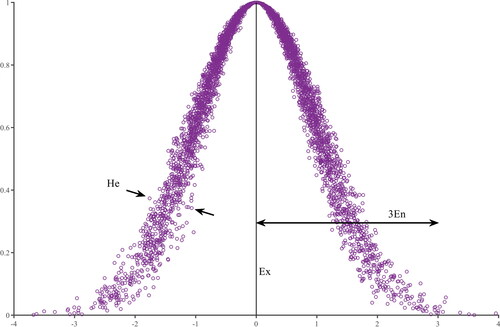
The cloud model, a conversion model that leverages concepts from probability theory and fuzzy logic to capture and quantify uncertainty between quality and quantity, was originally proposed by Li et al. in 2009. The cloud is composed of cloud droplets, each with a degree of certainty, indicating its probability of appearance (H.-C. Liu et al. 2019). The numerical parameters of a cloud are the expected value (Ex), entropy (En), and hyper entropy (He). Ex is the centre value within the domain of a given qualitative concept; En indicates ambiguity of the qualitative concept; and He quantifies the dispersion degree of a cloud droplet. The distribution of membership for a cloud model over the domain is called a membership cloud, or simply, a cloud. Normal cloud models are based on the normal distribution and Gaussian membership function (Li et al. 2009), with different applications, such as in energy (Zhao et al. 2020), air pollution evaluation (Peng and Wang 2018), risk evaluation (H.-C. Liu et al. 2019), group decision-making (P. Wang et al. 2018), and so forth.

Definition 1.

(Li and Du 2007). Let $T$ be a qualitative concept defined over the universe of discourse $U.$ A cloud droplet can be represented as $(x,y),$ where $x\in U$ is a random instantiation of the concept $T$ and $y\in [0,1]$ is the certainty degree of $x$ belonging to $T.$ Considering $x\sim N(\mathit{\text{Ex}},{\mathit{\text{En}}}^{\prime 2}),$ ${\mathit{\text{En}}}^{\prime }\sim N\left(\mathit{\text{En}},{\mathit{\text{He}}}^2\right)$ satisfied, the certainty degree can be calculated by Eq. (2)(2) $$y=\mathrm{\text{exp}}(-(x-\mathit{\text{Ex}}{)}^2/2{\mathit{\text{En}}}^{\prime 2})$$(2) , and the distribution of $x$ in $U$ is called a normal cloud. A normal cloud and its numerical characteristics are shown in Figure 1. (2) $$y=\mathrm{\text{exp}}(-(x-\mathit{\text{Ex}}{)}^2/2{\mathit{\text{En}}}^{\prime 2})$$(2)

Figure 1. Normal cloud.

Definition 2.

(H.-C. Liu et al. 2019). Consider a normal cloud $\tilde{y}=(\mathit{\text{Ex}},\mathit{\text{En}},\mathit{\text{He}})$ in the domain $U.$ Then we have: (3) $$\lambda \tilde{y}=\left(\lambda \mathit{\text{Ex}},\sqrt{\lambda }\mathit{\text{En}},\sqrt{\lambda }\mathit{\text{He}}\right),\lambda >0$$(3)

Definition 3.

(H.-C. Liu et al. 2019). Suppose any two normal clouds ${\tilde{y}}_1=({\mathit{\text{Ex}}}_1,{\mathit{\text{En}}}_1,{\mathit{\text{He}}}_1)$ and ${\tilde{y}}_2=({\mathit{\text{Ex}}}_2,{\mathit{\text{En}}}_2,{\mathit{\text{He}}}_2)$ in the domain of $U.$ We can convert the clouds into interval-values as ${\tilde{y}}_1\approx a=[\overline{a},\underset{¯}{a}]$ and ${\tilde{y}}_2\approx b=[\overline{b},\underset{¯}{b}],$ where $\overline{a}={\mathit{\text{Ex}}}_1+3{\mathit{\text{En}}}_1,$ $\underset{¯}{a}={\mathit{\text{Ex}}}_1-3{\mathit{\text{En}}}_1,$ $\overline{b}={\mathit{\text{Ex}}}_2+3{\mathit{\text{En}}}_2,$ and $\underset{¯}{b}=x_2-3{\mathit{\text{En}}}_2.$ Then, the two clouds can be compared using the following rules:

1. If $S_{{\tilde{y}}_1,{\tilde{y}}_2}>0,$ then ${\tilde{y}}_1>{\tilde{y}}_2;$

2. If $S_{{\tilde{y}}_1,{\tilde{y}}_2}=0$ and ${\mathit{\text{En}}}_1<{\mathit{\text{En}}}_2,$ then ${\tilde{y}}_1>{\tilde{y}}_2;$

3. If $S_{{\tilde{y}}_1,{\tilde{y}}_2}=0,$ ${\mathit{\text{En}}}_1={\mathit{\text{En}}}_2,$ and ${\mathit{\text{He}}}_1<{\mathit{\text{He}}}_2,$ then ${\tilde{y}}_1>{\tilde{y}}_2;$

4. If $\mathrm{ }{S}_{{\tilde{y}}_1,{\tilde{y}}_2}=0,$ ${\mathit{\text{En}}}_1={\mathit{\text{En}}}_2,$ and ${\mathit{\text{He}}}_1={\mathit{\text{He}}}_2,$ then ${\tilde{y}}_1={\tilde{y}}_2.$

Note that $\mathrm{ }{S}_{{\tilde{y}}_1,{\tilde{y}}_2}=2\left(\overline{a}-\underset{¯}{b}\right)-(\overline{a}-\underset{¯}{a}+\overline{b}-\underset{¯}{b}).$

Definition 4.

(Khorshidi and Aickelin 2021). Considering any two normal clouds ${\tilde{y}}_1=({\mathit{\text{Ex}}}_1,{\mathit{\text{En}}}_1,{\mathit{\text{He}}}_1)$ and ${\tilde{y}}_2=({\mathit{\text{Ex}}}_2,{\mathit{\text{En}}}_2,{\mathit{\text{He}}}_2),$ the distance between them is defined as Eq. (4)(4) $$d\left({\tilde{y}}_1,{\tilde{y}}_2\right)=\sqrt{{\left|{\mathit{\text{Ex}}}_1-{\mathit{\text{Ex}}}_2\right|}^2+\left|{\mathit{\text{En}}}_1-{\mathit{\text{En}}}_2\right|+\left|{\mathit{\text{He}}}_1-{\mathit{\text{He}}}_2\right|}$$(4) . (4) $$d\left({\tilde{y}}_1,{\tilde{y}}_2\right)=\sqrt{{\left|{\mathit{\text{Ex}}}_1-{\mathit{\text{Ex}}}_2\right|}^2+\left|{\mathit{\text{En}}}_1-{\mathit{\text{En}}}_2\right|+\left|{\mathit{\text{He}}}_1-{\mathit{\text{He}}}_2\right|}$$(4)

There are two methods for calculating the three parameters for the normal cloud (J. Wang et al. 2015). One is based on human experience, in which experts calculate the parameters, manually. The other is to define them using a cloud transformation method called the backward cloud generator. In this paper, we use the latter to aggregate decision-makers’ opinions. For this, we first determine the position of each cloud droplet using interval weights and then use the backward cloud generator to construct the cloud.

3. Proposed MCGDM

The proposed algorithm aims to (i) resolve the challenges regarding group decision-making using cloud models; (ii) provide a more straightforward data collection process, only reference pairwise comparisons will be used, guaranteeing more consistent data; and (iii) extract interval weights to cope with intra-expert uncertainty. The structure of the proposed method and its solutions to the challenges are given in Table 1.

The proposed approach makes two key contributions to group decision-making. Firstly, it addresses issues of sensitivity to outliers and lack of focus on opinion dispersion by utilising cloud models to aggregate opinions. Secondly, it seeks to minimise uncertainty in the decision-making process by employing interval values. To mitigate cognitive biases, the interval extraction process is designed to be indirect, where decision-makers only make pairwise comparisons and do not determine any intervals themselves. Sections 3.1 to 3.3 indicate the stages of the proposed approach.

3.1. Data collection

Sections 3.1.1 to Sections 3.1.4 indicate steps of the data collection stage, followed by a numerical example.

3.1.1. Determine the hierarchy decision model

Structure a decision hierarchy from the top with the goal of the decision, the criteria in the next level, and a set of alternatives at the lowest level of the hierarchy.

3.1.2. Determine references for pairwise comparison

For every criterion, considering the goal of the comparison, the most desirable (best) and the least desirable (worst) alternatives are determined.

3.1.3. Construct vector BO

Considering each criterion as the goal of the comparison, determine preference of the best alternative over all alternatives using a number between 1 and 9 – leading to calculation of the best-to-others (BO) vectors for each criterion.

3.1.4. Construct vector OW

Considering each criterion as the goal of the comparison, determine preference of all alternatives over the least important alternative using a number between 1 and 9 – resulting in the others-to-worst (OW) vectors to be computed for each criterion.

For instance, suppose that a group of decision-makers (D₁, D₂, and D₃) use three criteria (C₁, C₂, and C₃) to select the best alternative amongst four alternatives (A₁, A₂, A₃, and A₄). The output of stage 1 is summarised in Table 2.

Table 2. The output of stage 1.

Decision- maker ($D_k$)	Criteria ($C_j$)															References for pairwise comparison ($A_B^{\mathit{\text{kj}}},$ $A_W^{\mathit{\text{kj}}}$)
	C1					C2					C3
D1	BO	2	3	7	1	BO	3	1	2	8	BO	2	1	3	9	$A_B^{11}=A_4,A_W^{11}=A_3$ $A_B^{12}=A_2,A_W^{12}=A_1$ $A_B^{13}=A_2,A_W^{13}=A_4$
	OW	2	3	1	2	OW	1	5	2	3	OW	3	2	7	1
D2	BO	9	7	3	1	BO	4	1	8	5	BO	1	8	7	7	$A_B^{21}=A_4,A_W^{21}=A_1$ $A_B^{22}=A_2,A_W^{22}=A_3$ $A_B^{23}=A_1,A_W^{23}=A_2$
	OW	1	3	7	9	OW	5	9	1	4	OW	8	1	2	2
D3	BO	1	3	4	9	BO	7	1	2	4	BO	4	1	5	8	$A_B^{31}=A_1,A_W^{31}=A_4$ $A_B^{32}=A_2,A_W^{32}=A_1$ $A_B^{33}=A_2,A_W^{33}=A_4$
	OW	9	5	4	1	OW	1	7	4	6	OW	5	8	5	1

3.2. Interval weight matrix construction and aggregation

Sections 3.2.1 to 3.2.4 indicate the steps of the interval weight matrix construction and aggregation stage followed by a numerical example.

3.2.1. Find the optimal weights for alternatives against each criterion

Optimal weights for all alternatives against each criterion can be calculated by solving the following model for decision-maker k against criterion j: (5) $$\begin{array}{l}\mathrm{\text{min}}\mathrm{ }{e}_{\mathit{\text{kj}}}\\ s.t.\\ \begin{array}{l}\left|p_B^{\mathit{\text{kj}}}/p_i^{\mathit{\text{kj}}}-a_{\mathit{\text{Bi}}}^{\mathit{\text{kj}}}\right|\le e_{\mathit{\text{kj}}},\mathit{\text{for all}}\mathrm{ }i\\ \left|p_i^{\mathit{\text{kj}}}/p_W^{\mathit{\text{kj}}}-a_{\mathit{\text{iW}}}^{\mathit{\text{kj}}}\right|\le e_{\mathit{\text{kj}}},\mathit{\text{for all}}\mathrm{ }i\\ \sum _i{p}_i^{\mathit{\text{kj}}}=1,p_i^{\mathit{\text{kj}}}\ge 0\mathrm{ }\mathit{\text{for all}}\mathrm{ }i=1\text{to m}\end{array}\end{array}$$(5)

This model is formulated based on the Model (6) in Rezaei (2015), where $p_B^{\mathit{\text{kj}}}$ is the weight for the best alternative (B) against the criteria (j) on the basis of decision-maker (k) opinions, $p_W^{\mathit{\text{kj}}}$ is the weight for the worst alternative (W), and $p_i^{\mathit{\text{kj}}}$ is the weight for the alternative (i). The $a_{\mathit{\text{Bi}}}^{\mathit{\text{kj}}}$ is the value extracted from comparing the best alternative (B) with the alternative (i) against the criteria (j), based on decision-maker (k) opinion. Respectively, $a_{\mathit{\text{iW}}}^{\mathit{\text{kj}}}$ is the value extracted from comparing the alternative (i) against the criterion (j) with the worst alternative (W). The value of $e_{\mathit{\text{kj}}}$ refers to the amount of error occurred in the process of decision-making by decision-maker (k) against criteria (j).

By solving the problem in Eq. (5)(5) $$\begin{array}{l}\mathrm{\text{min}}\mathrm{ }{e}_{\mathit{\text{kj}}}\\ s.t.\\ \begin{array}{l}\left|p_B^{\mathit{\text{kj}}}/p_i^{\mathit{\text{kj}}}-a_{\mathit{\text{Bi}}}^{\mathit{\text{kj}}}\right|\le e_{\mathit{\text{kj}}},\mathit{\text{for all}}\mathrm{ }i\\ \left|p_i^{\mathit{\text{kj}}}/p_W^{\mathit{\text{kj}}}-a_{\mathit{\text{iW}}}^{\mathit{\text{kj}}}\right|\le e_{\mathit{\text{kj}}},\mathit{\text{for all}}\mathrm{ }i\\ \sum _i{p}_i^{\mathit{\text{kj}}}=1,p_i^{\mathit{\text{kj}}}\ge 0\mathrm{ }\mathit{\text{for all}}\mathrm{ }i=1\text{to m}\end{array}\end{array}$$(5) for each decision-maker, $P_k$ (Eq. (6)(6) $$\begin{gathered} P_k=\begin{array}{c}\begin{array}{cccc} C_1& C_2& \dots & C_n\end{array}\\ \begin{array}{c}{A}_1\\ A_2\\ ⋮\\ A_m\end{array}\left[\begin{array}{cccc}{p}_{11}& p_{12}& \dots & p_{1n}\\ p_{21}& p_{22}& \dots & p_{2n}\\ ⋮& ⋮& \ddots & ⋮\\ p_{m1}& p_{m2}& \dots & p_{\mathit{\text{mn}}}\end{array}\right]\end{array} \mathit{\text{for all}}\mathrm{ }k=1\text{to D} \\ {e}_k^{\mathrm{*}}=\left(\begin{array}{cccc}{e}_{k1}^{\mathrm{*}},& e_{k2}^{\mathrm{*}},& \cdots & e_{\mathit{\text{kj}}}^{\mathrm{*}}\end{array}\right)\hspace{0.5em}\mathit{\text{for all}}\mathrm{ }k=1\text{to D} \end{gathered}$$(6) ), the optimal weight matrix for decision-maker k, is calculated, where $p_{\mathit{\text{ij}}}$ denotes the optimal weight of alternative i against criterion j. (6) $$\begin{gathered} P_k=\begin{array}{c}\begin{array}{cccc} C_1& C_2& \dots & C_n\end{array}\\ \begin{array}{c}{A}_1\\ A_2\\ ⋮\\ A_m\end{array}\left[\begin{array}{cccc}{p}_{11}& p_{12}& \dots & p_{1n}\\ p_{21}& p_{22}& \dots & p_{2n}\\ ⋮& ⋮& \ddots & ⋮\\ p_{m1}& p_{m2}& \dots & p_{\mathit{\text{mn}}}\end{array}\right]\end{array} \mathit{\text{for all}}\mathrm{ }k=1\text{to D} \\ {e}_k^{\mathrm{*}}=\left(\begin{array}{cccc}{e}_{k1}^{\mathrm{*}},& e_{k2}^{\mathrm{*}},& \cdots & e_{\mathit{\text{kj}}}^{\mathrm{*}}\end{array}\right)\hspace{0.5em}\mathit{\text{for all}}\mathrm{ }k=1\text{to D} \end{gathered}$$(6)

3.2.2. Extract interval values

The models used in the prior step result in multiple optimal solutions for problems with the non-zero consistency ratio. Solving the problem in Eq. (7)(7) $$\begin{array}{l}\mathrm{\text{min}}\hspace{0.17em}{\mathit{\text{Lp}}}_i^{\mathit{\text{kj}}}\\ \mathrm{s}.\mathrm{t}.\\ \begin{array}{l}\left|{\mathit{\text{Lp}}}_B^{\mathit{\text{kj}}}/L{p}_i^{\mathit{\text{kj}}}-a_{\mathit{\text{Bi}}}^{\mathit{\text{kj}}}\right|\le e_{\mathit{\text{kj}}}^{\mathrm{*}},\mathit{\text{for all}}\mathrm{ }i\\ \begin{array}{l}\left|{\mathit{\text{Lp}}}_i^{\mathit{\text{kj}}}/L{p}_W^{\mathit{\text{kj}}}-a_{\mathit{\text{iW}}}^{\mathit{\text{kj}}}\right|\le e_{\mathit{\text{kj}}}^{\mathrm{*}},\mathit{\text{for all}}\mathrm{ }i\\ \sum _i{p}_i^{\mathit{\text{kj}}}=1,L{p}_i^{\mathit{\text{kj}}}\ge 0\mathrm{ }\mathit{\text{for all}}\mathrm{ }i=1\text{to m}\end{array}\end{array}\end{array}$$(7) , formulated based on the Model (5) in Rezaei (2015), for each decision-maker k against each criterion j gives the lower bounds for each $p_{\mathit{\text{ij}}}$ in $P_k$ matrix. (7) $$\begin{array}{l}\mathrm{\text{min}}\hspace{0.17em}{\mathit{\text{Lp}}}_i^{\mathit{\text{kj}}}\\ \mathrm{s}.\mathrm{t}.\\ \begin{array}{l}\left|{\mathit{\text{Lp}}}_B^{\mathit{\text{kj}}}/L{p}_i^{\mathit{\text{kj}}}-a_{\mathit{\text{Bi}}}^{\mathit{\text{kj}}}\right|\le e_{\mathit{\text{kj}}}^{\mathrm{*}},\mathit{\text{for all}}\mathrm{ }i\\ \begin{array}{l}\left|{\mathit{\text{Lp}}}_i^{\mathit{\text{kj}}}/L{p}_W^{\mathit{\text{kj}}}-a_{\mathit{\text{iW}}}^{\mathit{\text{kj}}}\right|\le e_{\mathit{\text{kj}}}^{\mathrm{*}},\mathit{\text{for all}}\mathrm{ }i\\ \sum _i{p}_i^{\mathit{\text{kj}}}=1,L{p}_i^{\mathit{\text{kj}}}\ge 0\mathrm{ }\mathit{\text{for all}}\mathrm{ }i=1\text{to m}\end{array}\end{array}\end{array}$$(7)

Upper bounds for each $p_{\mathit{\text{ij}}}$ in the $P_k$ matrix can be derived from solving the problem in Eq. (8)(8) $$\begin{array}{l}\mathrm{\text{max}}\mathrm{ }{\mathit{\text{Up}}}_i^{\mathit{\text{kj}}}\\ \mathrm{s}.\mathrm{t}.\\ \begin{array}{l}\left|{\mathit{\text{Up}}}_B^{\mathit{\text{kj}}}/U{p}_i^{\mathit{\text{kj}}}-a_{\mathit{\text{Bi}}}^{\mathit{\text{kj}}}\right|\le e_{\mathit{\text{kj}}}^{\mathrm{*}},\mathit{\text{for all}}\mathrm{ }i\\ \begin{array}{l}\left|{\mathit{\text{Up}}}_i^{\mathit{\text{kj}}}/U{p}_W^{\mathit{\text{kj}}}-a_{\mathit{\text{iW}}}^{\mathit{\text{kj}}}\right|\le e_{\mathit{\text{kj}}}^{\mathrm{*}},\mathit{\text{for all}}\mathrm{ }i\\ \sum _i{p}_i^{\mathit{\text{kj}}}=1,U{p}_i^{\mathit{\text{kj}}}\ge 0\mathrm{ }\mathit{\text{for all}}\mathrm{ }i=1\text{to m}\end{array}\end{array}\end{array}$$(8) , for each decision-maker k against each criterion j.(8) $$\begin{array}{l}\mathrm{\text{max}}\mathrm{ }{\mathit{\text{Up}}}_i^{\mathit{\text{kj}}}\\ \mathrm{s}.\mathrm{t}.\\ \begin{array}{l}\left|{\mathit{\text{Up}}}_B^{\mathit{\text{kj}}}/U{p}_i^{\mathit{\text{kj}}}-a_{\mathit{\text{Bi}}}^{\mathit{\text{kj}}}\right|\le e_{\mathit{\text{kj}}}^{\mathrm{*}},\mathit{\text{for all}}\mathrm{ }i\\ \begin{array}{l}\left|{\mathit{\text{Up}}}_i^{\mathit{\text{kj}}}/U{p}_W^{\mathit{\text{kj}}}-a_{\mathit{\text{iW}}}^{\mathit{\text{kj}}}\right|\le e_{\mathit{\text{kj}}}^{\mathrm{*}},\mathit{\text{for all}}\mathrm{ }i\\ \sum _i{p}_i^{\mathit{\text{kj}}}=1,U{p}_i^{\mathit{\text{kj}}}\ge 0\mathrm{ }\mathit{\text{for all}}\mathrm{ }i=1\text{to m}\end{array}\end{array}\end{array}$$(8)

This model is formulated based on the Model (6) in Rezaei (2015). Equation (9)(9) $${\mathit{\text{IP}}}_k=\begin{array}{c} \begin{array}{cccc}{C}_1& C_2& \cdots & C_n\end{array}\\ \begin{array}{c}{A}_1\\ A_2\\ ⋮\\ A_m\end{array}\left[\begin{array}{cccc}\left[\begin{array}{cc}{p}_{11}^L& p_{11}^U\end{array}\right]& \left[\begin{array}{cc}{p}_{12}^L& p_{12}^U\end{array}\right]& \dots & \left[\begin{array}{cc}{p}_{1n}^L& p_{1n}^U\end{array}\right]\\ \left[\begin{array}{cc}{p}_{21}^L& p_{21}^U\end{array}\right]& \left[\begin{array}{cc}{p}_{22}^L& p_{22}^U\end{array}\right]& \dots & \left[\begin{array}{cc}{p}_{2n}^L& p_{2n}^U\end{array}\right]\\ ⋮& ⋮& \ddots & ⋮\\ \left[\begin{array}{cc}{p}_{m1}^L& p_{m1}^U\end{array}\right]& \left[\begin{array}{cc}{p}_{m2}^L& p_{m2}^U\end{array}\right]& \dots & \left[\begin{array}{cc}{p}_{\mathit{\text{mn}}}^L& p_{\mathit{\text{mn}}}^U\end{array}\right]\end{array}\right]\end{array}$$(9) represents the resultant decision matrix obtained after calculating the lower and the upper bounds. (9) $${\mathit{\text{IP}}}_k=\begin{array}{c} \begin{array}{cccc}{C}_1& C_2& \cdots & C_n\end{array}\\ \begin{array}{c}{A}_1\\ A_2\\ ⋮\\ A_m\end{array}\left[\begin{array}{cccc}\left[\begin{array}{cc}{p}_{11}^L& p_{11}^U\end{array}\right]& \left[\begin{array}{cc}{p}_{12}^L& p_{12}^U\end{array}\right]& \dots & \left[\begin{array}{cc}{p}_{1n}^L& p_{1n}^U\end{array}\right]\\ \left[\begin{array}{cc}{p}_{21}^L& p_{21}^U\end{array}\right]& \left[\begin{array}{cc}{p}_{22}^L& p_{22}^U\end{array}\right]& \dots & \left[\begin{array}{cc}{p}_{2n}^L& p_{2n}^U\end{array}\right]\\ ⋮& ⋮& \ddots & ⋮\\ \left[\begin{array}{cc}{p}_{m1}^L& p_{m1}^U\end{array}\right]& \left[\begin{array}{cc}{p}_{m2}^L& p_{m2}^U\end{array}\right]& \dots & \left[\begin{array}{cc}{p}_{\mathit{\text{mn}}}^L& p_{\mathit{\text{mn}}}^U\end{array}\right]\end{array}\right]\end{array}$$(9)

The pseudo-code for constructing the interval weight matrix is presented in Algorithm 1.

Algorithm 1.

Interval weight matrix construction

Input: Vectors BO and OW for every criterion and each decision-maker, number of decision-makers D, number of criteria C, and number of alternatives A

Output: Interval weight matrix

1. for k from 1 to D do

2.  for j from 1 to C do

3.   for i from 1 to A do

4.$\hspace{1em}\hspace{1em}\hspace{1em}\hspace{1em}\hspace{1em}\hspace{1em}{e}_{\mathit{\text{kj}}}$ ← Determine the weight using Eq. (5)(5) $$\begin{array}{l}\mathrm{\text{min}}\mathrm{ }{e}_{\mathit{\text{kj}}}\\ s.t.\\ \begin{array}{l}\left|p_B^{\mathit{\text{kj}}}/p_i^{\mathit{\text{kj}}}-a_{\mathit{\text{Bi}}}^{\mathit{\text{kj}}}\right|\le e_{\mathit{\text{kj}}},\mathit{\text{for all}}\mathrm{ }i\\ \left|p_i^{\mathit{\text{kj}}}/p_W^{\mathit{\text{kj}}}-a_{\mathit{\text{iW}}}^{\mathit{\text{kj}}}\right|\le e_{\mathit{\text{kj}}},\mathit{\text{for all}}\mathrm{ }i\\ \sum _i{p}_i^{\mathit{\text{kj}}}=1,p_i^{\mathit{\text{kj}}}\ge 0\mathrm{ }\mathit{\text{for all}}\mathrm{ }i=1\text{to m}\end{array}\end{array}$$(5)

5.    end for

6.    for i from 1 to A do

7.$\hspace{1em}\hspace{1em}\hspace{1em}\hspace{1em}\hspace{1em}\hspace{1em}L{p}_{\mathit{\text{ij}}}$ ← Determine the lower bound of the weight using Eq. (7)(7) $$\begin{array}{l}\mathrm{\text{min}}\hspace{0.17em}{\mathit{\text{Lp}}}_i^{\mathit{\text{kj}}}\\ \mathrm{s}.\mathrm{t}.\\ \begin{array}{l}\left|{\mathit{\text{Lp}}}_B^{\mathit{\text{kj}}}/L{p}_i^{\mathit{\text{kj}}}-a_{\mathit{\text{Bi}}}^{\mathit{\text{kj}}}\right|\le e_{\mathit{\text{kj}}}^{\mathrm{*}},\mathit{\text{for all}}\mathrm{ }i\\ \begin{array}{l}\left|{\mathit{\text{Lp}}}_i^{\mathit{\text{kj}}}/L{p}_W^{\mathit{\text{kj}}}-a_{\mathit{\text{iW}}}^{\mathit{\text{kj}}}\right|\le e_{\mathit{\text{kj}}}^{\mathrm{*}},\mathit{\text{for all}}\mathrm{ }i\\ \sum _i{p}_i^{\mathit{\text{kj}}}=1,L{p}_i^{\mathit{\text{kj}}}\ge 0\mathrm{ }\mathit{\text{for all}}\mathrm{ }i=1\text{to m}\end{array}\end{array}\end{array}$$(7)

8. $\hspace{1em}\hspace{1em}\hspace{1em}\hspace{1em}\hspace{1em}\hspace{1em}U{p}_{\mathit{\text{ij}}}$ ← Determine the upper bound of the weight using Eq. (8)(8) $$\begin{array}{l}\mathrm{\text{max}}\mathrm{ }{\mathit{\text{Up}}}_i^{\mathit{\text{kj}}}\\ \mathrm{s}.\mathrm{t}.\\ \begin{array}{l}\left|{\mathit{\text{Up}}}_B^{\mathit{\text{kj}}}/U{p}_i^{\mathit{\text{kj}}}-a_{\mathit{\text{Bi}}}^{\mathit{\text{kj}}}\right|\le e_{\mathit{\text{kj}}}^{\mathrm{*}},\mathit{\text{for all}}\mathrm{ }i\\ \begin{array}{l}\left|{\mathit{\text{Up}}}_i^{\mathit{\text{kj}}}/U{p}_W^{\mathit{\text{kj}}}-a_{\mathit{\text{iW}}}^{\mathit{\text{kj}}}\right|\le e_{\mathit{\text{kj}}}^{\mathrm{*}},\mathit{\text{for all}}\mathrm{ }i\\ \sum _i{p}_i^{\mathit{\text{kj}}}=1,U{p}_i^{\mathit{\text{kj}}}\ge 0\mathrm{ }\mathit{\text{for all}}\mathrm{ }i=1\text{to m}\end{array}\end{array}\end{array}$$(8)

9.    end for

10.  end for

11.  ${\mathit{\text{IP}}}_k$ ← Construct the interval weight matrix for each decision-maker k

12. end for

3.2.3. Aggregate the opinions of decision makers

Equation (10)(10) $$\{\begin{array}{c}\mathit{\text{Ex}}=\frac{1}{D}\sum _k{\overline{x}}_k \\ \mathit{\text{En}}=\frac{1}{D}\sum _k{\sigma }_k+\sqrt{\frac{1}{D}\sum _k({\overline{x}}_k-\mathit{\text{Ex}}{)}^2}\\ \mathit{\text{He}}=\sqrt{\frac{1}{D}\sum _k({\sigma }_k-\mathit{\text{En}}{)}^2} \end{array}$$(10) can be used to aggregate the interval-values of each decision-maker’s opinion and translate them into cloud models: (10) $$\{\begin{array}{c}\mathit{\text{Ex}}=\frac{1}{D}\sum _k{\overline{x}}_k \\ \mathit{\text{En}}=\frac{1}{D}\sum _k{\sigma }_k+\sqrt{\frac{1}{D}\sum _k({\overline{x}}_k-\mathit{\text{Ex}}{)}^2}\\ \mathit{\text{He}}=\sqrt{\frac{1}{D}\sum _k({\sigma }_k-\mathit{\text{En}}{)}^2} \end{array}$$(10)

Where, for each interval-value such as I = $\left[p_{\mathit{\text{ij}}}^L,p_{\mathit{\text{ij}}}^U\right]:$ (11) $$\{\begin{array}{c}\overline{x}=(p_{\mathit{\text{ij}}}^L+p_{\mathit{\text{ij}}}^U)/2\\ \sigma =(p_{\mathit{\text{ij}}}^U-p_{\mathit{\text{ij}}}^L)/6\end{array}$$(11)

3.2.4. Constructing decision cloud matrix

After aggregating the interval-values, there will be a cloud model for each criterion of each alternative, denoted by ${\tilde{y}}_{\mathit{\text{ij}}}=\left({\mathit{\text{Ex}}}_{\mathit{\text{ij}}},{\mathit{\text{En}}}_{\mathit{\text{ij}}},{\mathit{\text{He}}}_{\mathit{\text{ij}}}\right).$ The decision cloud matrix $\tilde{Y}$ can be constructed as follow: (12) $$\tilde{Y}=\begin{array}{c} \begin{array}{cccc}{C}_1& C_2& \cdots & C_n\end{array}\\ \begin{array}{c}{A}_1\\ A_2\\ ⋮\\ A_m\end{array}\left[\begin{array}{cccc}{\tilde{y}}_{11}& {\tilde{y}}_{12}& \cdots & {\tilde{y}}_{1n}\\ {\tilde{y}}_{21}& {\tilde{y}}_{22}& \cdots & {\tilde{y}}_{2n}\\ ⋮& ⋮& \ddots & ⋮\\ {\tilde{y}}_{m1}& {\tilde{y}}_{m2}& \cdots & {\tilde{y}}_{\mathit{\text{mn}}}\end{array}\right]\end{array}$$(12)

The pseudo-code for constructing a cloud decision matrix is given in Algorithm 2.

Algorithm 2.

Cloud decision matrix construction

Input: Interval weight matrix

Output: Cloud decision matrix

1. for k from 1 to D do

2.  for j from 1 to C do

3.   for i from 1 to A do

4.     ${\overline{x}}_{\mathit{\text{ij}}}^k$ ← Determine the mean using Eq. (11)(11) $$\{\begin{array}{c}\overline{x}=(p_{\mathit{\text{ij}}}^L+p_{\mathit{\text{ij}}}^U)/2\\ \sigma =(p_{\mathit{\text{ij}}}^U-p_{\mathit{\text{ij}}}^L)/6\end{array}$$(11)

5.     ${\sigma }_{\mathit{\text{ij}}}^k$ ← Determine the standard deviation using Eq. (11)(11) $$\{\begin{array}{c}\overline{x}=(p_{\mathit{\text{ij}}}^L+p_{\mathit{\text{ij}}}^U)/2\\ \sigma =(p_{\mathit{\text{ij}}}^U-p_{\mathit{\text{ij}}}^L)/6\end{array}$$(11)

6.   end for

7.  end for

8. end for

9.  for i from 1 to A do

10.   for j from 1 to C do

11.     ${\mathit{\text{Ex}}}_{\mathit{\text{ij}}}$ ← Calculate the expectation of the aggregated cloud using Eq. (10)(10) $$\{\begin{array}{c}\mathit{\text{Ex}}=\frac{1}{D}\sum _k{\overline{x}}_k \\ \mathit{\text{En}}=\frac{1}{D}\sum _k{\sigma }_k+\sqrt{\frac{1}{D}\sum _k({\overline{x}}_k-\mathit{\text{Ex}}{)}^2}\\ \mathit{\text{He}}=\sqrt{\frac{1}{D}\sum _k({\sigma }_k-\mathit{\text{En}}{)}^2} \end{array}$$(10)

12.     ${\mathit{\text{En}}}_{\mathit{\text{ij}}}$ ← Calculate the entropy of the aggregated cloud using Eq. (10)(10) $$\{\begin{array}{c}\mathit{\text{Ex}}=\frac{1}{D}\sum _k{\overline{x}}_k \\ \mathit{\text{En}}=\frac{1}{D}\sum _k{\sigma }_k+\sqrt{\frac{1}{D}\sum _k({\overline{x}}_k-\mathit{\text{Ex}}{)}^2}\\ \mathit{\text{He}}=\sqrt{\frac{1}{D}\sum _k({\sigma }_k-\mathit{\text{En}}{)}^2} \end{array}$$(10)

13.     ${\mathit{\text{He}}}_{\mathit{\text{ij}}}$ ← Calculate the hyper-entropy of the aggregated cloud using Eq. (10)(10) $$\{\begin{array}{c}\mathit{\text{Ex}}=\frac{1}{D}\sum _k{\overline{x}}_k \\ \mathit{\text{En}}=\frac{1}{D}\sum _k{\sigma }_k+\sqrt{\frac{1}{D}\sum _k({\overline{x}}_k-\mathit{\text{Ex}}{)}^2}\\ \mathit{\text{He}}=\sqrt{\frac{1}{D}\sum _k({\sigma }_k-\mathit{\text{En}}{)}^2} \end{array}$$(10)

14.     ${\tilde{y}}_{\mathit{\text{ij}}} \text{←} \left({\mathit{\text{Ex}}}_{\mathit{\text{ij}}},{\mathit{\text{En}}}_{\mathit{\text{ij}}},{\mathit{\text{He}}}_{\mathit{\text{ij}}}\right)$

15.   end for

16. end for

17. $\tilde{Y}$ ← Construct the cloud decision matrix by ${\tilde{y}}_{\mathit{\text{ij}}}=\left({\mathit{\text{Ex}}}_{\mathit{\text{ij}}},{\mathit{\text{En}}}_{\mathit{\text{ij}}},{\mathit{\text{He}}}_{\mathit{\text{ij}}}\right)$

As another illustrative example and by means of the same data as those applied following Section 3.1, optimal weights are calculated by solving Eq. (5)(5) $$\begin{array}{l}\mathrm{\text{min}}\mathrm{ }{e}_{\mathit{\text{kj}}}\\ s.t.\\ \begin{array}{l}\left|p_B^{\mathit{\text{kj}}}/p_i^{\mathit{\text{kj}}}-a_{\mathit{\text{Bi}}}^{\mathit{\text{kj}}}\right|\le e_{\mathit{\text{kj}}},\mathit{\text{for all}}\mathrm{ }i\\ \left|p_i^{\mathit{\text{kj}}}/p_W^{\mathit{\text{kj}}}-a_{\mathit{\text{iW}}}^{\mathit{\text{kj}}}\right|\le e_{\mathit{\text{kj}}},\mathit{\text{for all}}\mathrm{ }i\\ \sum _i{p}_i^{\mathit{\text{kj}}}=1,p_i^{\mathit{\text{kj}}}\ge 0\mathrm{ }\mathit{\text{for all}}\mathrm{ }i=1\text{to m}\end{array}\end{array}$$(5) ; interval-valued data are extracted via Eqs. (7)(7) $$\begin{array}{l}\mathrm{\text{min}}\hspace{0.17em}{\mathit{\text{Lp}}}_i^{\mathit{\text{kj}}}\\ \mathrm{s}.\mathrm{t}.\\ \begin{array}{l}\left|{\mathit{\text{Lp}}}_B^{\mathit{\text{kj}}}/L{p}_i^{\mathit{\text{kj}}}-a_{\mathit{\text{Bi}}}^{\mathit{\text{kj}}}\right|\le e_{\mathit{\text{kj}}}^{\mathrm{*}},\mathit{\text{for all}}\mathrm{ }i\\ \begin{array}{l}\left|{\mathit{\text{Lp}}}_i^{\mathit{\text{kj}}}/L{p}_W^{\mathit{\text{kj}}}-a_{\mathit{\text{iW}}}^{\mathit{\text{kj}}}\right|\le e_{\mathit{\text{kj}}}^{\mathrm{*}},\mathit{\text{for all}}\mathrm{ }i\\ \sum _i{p}_i^{\mathit{\text{kj}}}=1,L{p}_i^{\mathit{\text{kj}}}\ge 0\mathrm{ }\mathit{\text{for all}}\mathrm{ }i=1\text{to m}\end{array}\end{array}\end{array}$$(7) and (8)(8) $$\begin{array}{l}\mathrm{\text{max}}\mathrm{ }{\mathit{\text{Up}}}_i^{\mathit{\text{kj}}}\\ \mathrm{s}.\mathrm{t}.\\ \begin{array}{l}\left|{\mathit{\text{Up}}}_B^{\mathit{\text{kj}}}/U{p}_i^{\mathit{\text{kj}}}-a_{\mathit{\text{Bi}}}^{\mathit{\text{kj}}}\right|\le e_{\mathit{\text{kj}}}^{\mathrm{*}},\mathit{\text{for all}}\mathrm{ }i\\ \begin{array}{l}\left|{\mathit{\text{Up}}}_i^{\mathit{\text{kj}}}/U{p}_W^{\mathit{\text{kj}}}-a_{\mathit{\text{iW}}}^{\mathit{\text{kj}}}\right|\le e_{\mathit{\text{kj}}}^{\mathrm{*}},\mathit{\text{for all}}\mathrm{ }i\\ \sum _i{p}_i^{\mathit{\text{kj}}}=1,U{p}_i^{\mathit{\text{kj}}}\ge 0\mathrm{ }\mathit{\text{for all}}\mathrm{ }i=1\text{to m}\end{array}\end{array}\end{array}$$(8) ; and the result is the interval weight matrices for each decision-maker (Table 3).

Table 3. Optimal weights and the interval weight matrices.

($D_k$)	Optimal weights	Interval weight matrix
D1	$P_1=\left[\begin{array}{ccc}\left(0.2231\right)& \left(0.1079\right)& \left(0.1818\right)\\ \left(0.2315\right)& \left(0.5530\right)& \left(0.3333\right)\\ \left(0.0992\right)& \left(0.2449\right)& \left(0.4242\right)\\ \left(0.4462\right)& \left(0.0942\right)& \left(0.0606\right)\end{array}\right]$	${\mathit{\text{IP}}}_1=\left[\begin{array}{ccc}\left(0.0833,0.2363\right)& \left(0.0899,0.1213\right)& \left(0.0556,0.3939\right)\\ \left(0.0756,0.4583\right)& \left(0.4608,0.6220\right)& \left(0.2340,0.4999\right)\\ \left(0.0645,0.1035\right)& \left(0.1507,0.3709\right)& \left(0.2121,0.5833\right)\\ \left(0.2903,0.6149\right)& \left(0.0785,0.1059\right)& \left(0.0426,0.0733\right)\end{array}\right]$
D2	$P_2=\left[\begin{array}{ccc}\left(0.0533\right)& \left(0.2171\right)& \left(0.6992\right)\\ \left(0.0944\right)& \left(0.5657\right)& \left(0.0809\right)\\ \left(0.3075\right)& \left(0.0602\right)& \left(0.1100\right)\\ \left(0.5449\right)& \left(0.1569\right)& \left(0.1100\right)\end{array}\right]$	${\mathit{\text{IP}}}_2=\left[\begin{array}{ccc}(0.0533,0.0533)& (0.2171,0.2171)& (0.6992,0.6992)\\ (0.0944,0.0944)& (0.5657,0.5657)& (0.0809,0.0809)\\ (0.3075,0.3075)& (0.0602,0.0602)& (0.1100,0.1100)\\ (0.5449,0.5449)& (0.1569,0.1569)& (0.1100,0.1100)\end{array}\right]$
D3	$P_3=\left[\begin{array}{ccc}\left(0.5164\right)& \left(0.0556\right)& \left(0.2139\right)\\ \left(0.2586\right)& \left(0.4922\right)& \left(0.5536\right)\\ \left(0.1676\right)& \left(0.2222\right)& \left(0.1763\right)\\ \left(0.0574\right)& \left(0.2300\right)& \left(0.0562\right)\end{array}\right]$	${\mathit{\text{IP}}}_3=\left[\begin{array}{ccc}\left(0.4615,0.5950\right)& \left(0.0504,0.0614\right)& \left(0.2090,0.2476\right)\\ \left(0.1862,0.3219\right)& \left(0.4461,0.5437\right)& \left(0.5299,0.5753\right)\\ \left(0.1668,0.2142\right)& \left(0.1409,0.2391\right)& \left(0.1688,0.1832\right)\\ \left(0.0455,0.0682\right)& \left(0.2206,0.2300\right)& \left(0.0561,0.0583\right)\end{array}\right]$

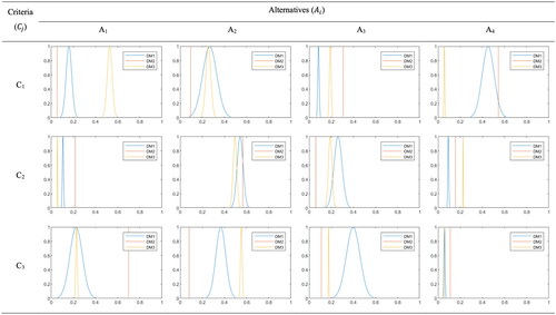
Intervals are visualized in Figure 2. Also, Gaussian membership functions (GMF) for decision-makers are presented in Figure 3. The range of the interval weights and the range of GMFs represent decision-makers’ uncertainty. It is shown that a less certain opinion results in a larger range of interval weights and a larger GMF range. In this example, D₂ has certain opinions. The range of the interval weights and the GMFs for this decision-maker are close to zero. In contrast, D₁ has the most uncertain opinions amongst other decision-makers, and consequently the ranges are larger than others.

Figure 2. Extracted interval weights.

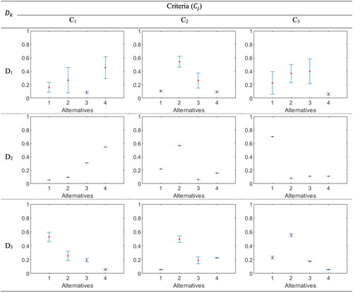
Figure 3. Gaussian membership functions (GMF) for decision-makers.

An estimation for each interval ($\overline{x}$) and the uncertainty of this estimation ($\sigma$) can be calculated using Eq. (11)(11) $$\{\begin{array}{c}\overline{x}=(p_{\mathit{\text{ij}}}^L+p_{\mathit{\text{ij}}}^U)/2\\ \sigma =(p_{\mathit{\text{ij}}}^U-p_{\mathit{\text{ij}}}^L)/6\end{array}$$(11) , as shown in Table 4. Once the interval values are converted into a pair as ($\overline{x},$ $\sigma$), we can use Eq. (10)(10) $$\{\begin{array}{c}\mathit{\text{Ex}}=\frac{1}{D}\sum _k{\overline{x}}_k \\ \mathit{\text{En}}=\frac{1}{D}\sum _k{\sigma }_k+\sqrt{\frac{1}{D}\sum _k({\overline{x}}_k-\mathit{\text{Ex}}{)}^2}\\ \mathit{\text{He}}=\sqrt{\frac{1}{D}\sum _k({\sigma }_k-\mathit{\text{En}}{)}^2} \end{array}$$(10) to aggregate the opinions and construct the clouds. The result of this aggregation is shown in Table 5. The $\mathit{\text{Ex}}$ in each aggregated cloud is calculated using the average of estimation values of intervals, which represents centre value of cloud drops. In each aggregated cloud, there are two sources of uncertainty that makes the entropy: (i) the average of estimation uncertainty ($\sigma$); and the variation of interval estimations ($\overline{x}$) from the $\mathit{\text{Ex}}.$ The latter, in an aggregated cloud, is the hyper-entropy, showing the level of uncertainty dispersion across decision-makers.

Table 4. Interval weight matrices and the cloud decision matrix.

($D_k$)	Estimations of each intervals (${\overline{x}}_k$)	Uncertainty of the estimation (${\sigma }_k$)
D1	${\overline{x}}_1=\left[\begin{array}{ccc}\left(0.1598\right)& \left(0.1056\right)& \left(0.2247\right)\\ \left(0.2670\right)& \left(0.5414\right)& \left(0.3670\right)\\ \left(0.0840\right)& \left(0.2608\right)& \left(0.3977\right)\\ \left(0.4526\right)& \left(0.0922\right)& \left(0.0579\right)\end{array}\right]$	${\sigma }_1=\left[\begin{array}{ccc}\left(0.0255\right)& \left(0.0052\right)& \left(0.0564\right)\\ \left(0.0638\right)& \left(0.0269\right)& \left(0.0443\right)\\ \left(0.0065\right)& \left(0.0367\right)& \left(0.0619\right)\\ \left(0.0541\right)& \left(0.0046\right)& \left(0.0051\right)\end{array}\right]$
D2	${\overline{x}}_2=\left[\begin{array}{ccc}\left(0.0533\right)& \left(0.2171\right)& \left(0.6992\right)\\ \left(0.0944\right)& \left(0.5657\right)& \left(0.0809\right)\\ \left(0.3075\right)& \left(0.0602\right)& \left(0.1100\right)\\ \left(0.5449\right)& \left(0.1569\right)& \left(0.1100\right)\end{array}\right]$	${\sigma }_2=\left[\begin{array}{ccc}\left(0.00\right)& \left(0.00\right)& \left(0.00\right)\\ \left(0.00\right)& \left(0.00\right)& \left(0.00\right)\\ \left(0.00\right)& \left(0.00\right)& \left(0.00\right)\\ \left(0.00\right)& \left(0.00\right)& \left(0.00\right)\end{array}\right]$
D3	${\overline{x}}_3=\left[\begin{array}{ccc}\left(0.5282\right)& \left(0.0559\right)& \left(0.2283\right)\\ \left(0.2541\right)& \left(0.4949\right)& \left(0.5526\right)\\ \left(0.1905\right)& \left(0.1900\right)& \left(0.1760\right)\\ \left(0.0568\right)& \left(0.2253\right)& \left(0.0572\right)\end{array}\right]$	${\sigma }_3=\left[\begin{array}{ccc}\left(0.0222\right)& \left(0.0018\right)& \left(0.0064\right)\\ \left(0.0226\right)& \left(0.0163\right)& \left(0.0076\right)\\ \left(0.0079\right)& \left(0.0164\right)& \left(0.0024\right)\\ \left(0.0038\right)& \left(0.0016\right)& \left(0.0004\right)\end{array}\right]$

Table 5. Cloud decision matrix.

$\tilde{Y}$	C1	C2	C3
A1	$(0.2471,0.2194,0.2038)$	$(0.1262,0.0698,0.0675)$	$(0.3841,0.2438,0.2242)$
A2	$(0.2051,0.1073,0.0828)$	$(0.5340,0.0438,0.0314)$	$(0.3335,0.2113,0.1950)$
A3	$(0.1940,0.0961,0.0913)$	$(0.1703,0.1008,0.0844)$	$(0.2279,0.1445,0.1264)$
A4	$(0.3514,0.2310,0.2131)$	$(0.1581,0.0564,0.0544)$	$(0.0750,0.0265,0.0248)$

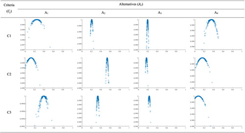
As shown in Figure 4, cloud droplets in each aggregated cloud are concentrated around the $\mathit{\text{Ex}}$ and scattered across the domain based on decision-makers’ uncertainty. The uncertainty level is at the lowest level for C₃A₄. The reason is that the decision-makers are in more agreement, with all of whom being relatively certain about their opinions (see C₃A₄ also in Figure 3). The aggregated cloud C₃A₁ has the highest level of uncertainty as both its entropy and hyper-entropy are highest. This uncertainty originates from the dispersed uncertainties across decision-makers, the large range of GMF for D₁, and the dispersion of estimated values form the $\mathit{\text{Ex}}.$

Figure 4. Aggregated cloud decision matrix.

3.3. Prioritisation

Sections 3.3.1 to 3.3.5 indicate steps of the prioritisation stage, followed by a numerical example.

3.3.1. Determine weights of criteria

After obtaining the decision cloud matrix, the weights for criteria can be determined using the hyper-entropy of cloud models. Due to the importance of the agreement level amongst decision-makers in a group decision-making process, we use the bi-level optimisation model proposed by Khorshidi and Aickelin (2021) to weight the criteria. Using this model, the criterion with a higher level of agreement amongst decision-makers gets a higher weight. This can help the decision-making process become more robust and less sensitive to the variation of opinions (Khorshidi and Aickelin 2021). So, the optimal weights can be obtained by solving the bi-level optimisation (Eq. 13(13) $$\begin{array}{l}\mathit{\text{min}}\underset{\mathit{\text{ij}}}{\mathrm{\text{max}}}\left\{\left|{\mathit{\text{He}}}_{\mathit{\text{ij}}}{w}_j-{\mathit{\text{He}}}_{\mathit{\text{ijo}}}{w}_{\mathit{\text{jo}}}\right|\right\}\\ \mathrm{s}.\mathrm{t}.\\ \begin{array}{c}\sum _j{w}_j=1\\ w_j\ge 0,\mathit{\text{for all}}\mathrm{ }j\end{array}\end{array}$$(13) ). (13) $$\begin{array}{l}\mathit{\text{min}}\underset{\mathit{\text{ij}}}{\mathrm{\text{max}}}\left\{\left|{\mathit{\text{He}}}_{\mathit{\text{ij}}}{w}_j-{\mathit{\text{He}}}_{\mathit{\text{ijo}}}{w}_{\mathit{\text{jo}}}\right|\right\}\\ \mathrm{s}.\mathrm{t}.\\ \begin{array}{c}\sum _j{w}_j=1\\ w_j\ge 0,\mathit{\text{for all}}\mathrm{ }j\end{array}\end{array}$$(13)

In this bi-level optimisation model, the weight for the jth criterion is denoted by ‘w_j’ and ‘jo’ represents a specific criterion. The aim is to assign lower weights to criteria with higher hyper-entropy (i.e. greater dispersion) across all alternatives. This is because the criteria on which decision-makers have a higher level of agreement are considered more crucial in ranking alternatives, as they are deemed more reliable for the decision-making process. Conversely, criteria with higher uncertainty in collective opinion are assigned lower importance weights.

3.3.2. Construct the weighted decision cloud matrix

After obtaining the optimal weights for the criteria, the weighted decision cloud matrix is constructed by multiplying the optimal weights and the elements of the matrix (Eq. (14)(14) $${\widehat{\tilde{y}}}_{\mathit{\text{ij}}}={\tilde{y}}_{\mathit{\text{ij}}}\times w_j,\mathit{\text{for all}} i \mathit{\text{and}} j$$(14) ). (14) $${\widehat{\tilde{y}}}_{\mathit{\text{ij}}}={\tilde{y}}_{\mathit{\text{ij}}}\times w_j,\mathit{\text{for all}} i \mathit{\text{and}} j$$(14)

The result will be the matrix $\widehat{\tilde{Y}},$ with ${\widehat{\tilde{y}}}_{\mathit{\text{ij}}}$ denoting the elements of the weighted decision cloud matrix. (15) $$\widehat{\tilde{Y}}=\begin{array}{c}\begin{array}{cccc} C_1& C_2& \cdots & C_n\end{array}\\ \begin{array}{c}{A}_1\\ A_2\\ ⋮\\ A_m\end{array}\left[\begin{array}{cccc}{\widehat{\tilde{y}}}_{11}& {\widehat{\tilde{y}}}_{12}& \cdots & {\widehat{\tilde{y}}}_{1n}\\ {\widehat{\tilde{y}}}_{21}& {\widehat{\tilde{y}}}_{22}& \cdots & {\widehat{\tilde{y}}}_{2n}\\ ⋮& ⋮& \ddots & ⋮\\ {\widehat{\tilde{y}}}_{m1}& {\widehat{\tilde{y}}}_{m2}& \cdots & {\widehat{\tilde{y}}}_{\mathit{\text{mn}}}\end{array}\right]\end{array}$$(15)

3.3.3. Define the ideal solutions

As all the data we use for the decision-making are extracted from pairwise comparisons conducted in Section 3.1, it is safe to say that all the values are higher-the-better. Therefore, the Cloud Positive Ideal Solution (CPIS) and the Cloud Negative Ideal Solutions (CNIS) can be obtained using Eqs. (16)(16) $$\mathit{\text{CPIS}}=A^{+}=\left\{\underset{i}{\mathrm{\text{max}}}{\widehat{\tilde{y}}}_{\mathit{\text{ij}}},\forall j=1,\dots ,n\right\}=\left\{{\widehat{\tilde{y}}}_1^{+},{\widehat{\tilde{y}}}_2^{+},\dots ,{\widehat{\tilde{y}}}_n^{+}\right\}$$(16) and (17)(17) $$\mathit{\text{CNIS}}=A^{-}=\left\{\underset{i}{\mathrm{\text{min}}}{\widehat{\tilde{y}}}_{\mathit{\text{ij}}},\forall j=1,\dots ,n\right\}=\left\{{\widehat{\tilde{y}}}_1^{-},{\widehat{\tilde{y}}}_2^{-},\dots ,{\widehat{\tilde{y}}}_n^{-}\right\}$$(17) , respectively. (16) $$\mathit{\text{CPIS}}=A^{+}=\left\{\underset{i}{\mathrm{\text{max}}}{\widehat{\tilde{y}}}_{\mathit{\text{ij}}},\forall j=1,\dots ,n\right\}=\left\{{\widehat{\tilde{y}}}_1^{+},{\widehat{\tilde{y}}}_2^{+},\dots ,{\widehat{\tilde{y}}}_n^{+}\right\}$$(16) (17) $$\mathit{\text{CNIS}}=A^{-}=\left\{\underset{i}{\mathrm{\text{min}}}{\widehat{\tilde{y}}}_{\mathit{\text{ij}}},\forall j=1,\dots ,n\right\}=\left\{{\widehat{\tilde{y}}}_1^{-},{\widehat{\tilde{y}}}_2^{-},\dots ,{\widehat{\tilde{y}}}_n^{-}\right\}$$(17)

3.3.4. Calculate the distance from ideal solutions

The distance between the ideal solutions and each alternative is calculated based on Eq. (4)(4) $$d\left({\tilde{y}}_1,{\tilde{y}}_2\right)=\sqrt{{\left|{\mathit{\text{Ex}}}_1-{\mathit{\text{Ex}}}_2\right|}^2+\left|{\mathit{\text{En}}}_1-{\mathit{\text{En}}}_2\right|+\left|{\mathit{\text{He}}}_1-{\mathit{\text{He}}}_2\right|}$$(4) and using Eqs. (18)(18) $$d_i^{+}=\sum _{j}d\left({\widehat{\tilde{y}}}_{\mathit{\text{ij}}},{\widehat{\tilde{y}}}_j^{+}\right),\mathit{\text{for all}} i$$(18) and (19)(19) $$d_i^{-}=\sum _{j}d\left({\widehat{\tilde{y}}}_{\mathit{\text{ij}}},{\widehat{\tilde{y}}}_j^{-}\right),\mathit{\text{for all}} i$$(19) . (18) $$d_i^{+}=\sum _{j}d\left({\widehat{\tilde{y}}}_{\mathit{\text{ij}}},{\widehat{\tilde{y}}}_j^{+}\right),\mathit{\text{for all}} i$$(18) (19) $$d_i^{-}=\sum _{j}d\left({\widehat{\tilde{y}}}_{\mathit{\text{ij}}},{\widehat{\tilde{y}}}_j^{-}\right),\mathit{\text{for all}} i$$(19)

3.3.5. Determine the ranking score

The ranking order of each alternative $A_i$ can be determined using the ranking score ${\mathit{\text{RS}}}_i$ (Eq. (20)(20) $${\mathit{\text{RS}}}_i=\frac{d_i^{-}}{d_i^{-}+d_i^{+}},\mathit{\text{for all}} i$$(20) ). (20) $${\mathit{\text{RS}}}_i=\frac{d_i^{-}}{d_i^{-}+d_i^{+}},\mathit{\text{for all}} i$$(20)

Where the ${0\le \mathit{\text{RS}}}_i\le 1$ indicates the range, and the bigger value of ${\mathit{\text{RS}}}_i$ shows the more importance of the alternative $A_i.$ Accordingly, the ranking order of each alternative can be determined regarding their ${\mathit{\text{RS}}}_i$ in a descending order.

Algorithm 3.

Prioritisation

Input: Cloud decision matrix

Output: The ranking order of the alternatives

1. for j from 1 to C do

2.   $w_j$ ← Determine the weights for each criterion using Eq. (13)(13) $$\begin{array}{l}\mathit{\text{min}}\underset{\mathit{\text{ij}}}{\mathrm{\text{max}}}\left\{\left|{\mathit{\text{He}}}_{\mathit{\text{ij}}}{w}_j-{\mathit{\text{He}}}_{\mathit{\text{ijo}}}{w}_{\mathit{\text{jo}}}\right|\right\}\\ \mathrm{s}.\mathrm{t}.\\ \begin{array}{c}\sum _j{w}_j=1\\ w_j\ge 0,\mathit{\text{for all}}\mathrm{ }j\end{array}\end{array}$$(13)

3. end for

4. Construct the weighted decision cloud matrix using Eqs. (3)(3) $$\lambda \tilde{y}=\left(\lambda \mathit{\text{Ex}},\sqrt{\lambda }\mathit{\text{En}},\sqrt{\lambda }\mathit{\text{He}}\right),\lambda >0$$(3) and (13)(13) $$\begin{array}{l}\mathit{\text{min}}\underset{\mathit{\text{ij}}}{\mathrm{\text{max}}}\left\{\left|{\mathit{\text{He}}}_{\mathit{\text{ij}}}{w}_j-{\mathit{\text{He}}}_{\mathit{\text{ijo}}}{w}_{\mathit{\text{jo}}}\right|\right\}\\ \mathrm{s}.\mathrm{t}.\\ \begin{array}{c}\sum _j{w}_j=1\\ w_j\ge 0,\mathit{\text{for all}}\mathrm{ }j\end{array}\end{array}$$(13)

5. for j from 1 to C do

6.   ${\widehat{\tilde{y}}}_j^{+}$ ← Determine the cloud positive ideal solution using Eq. (16)(16) $$\mathit{\text{CPIS}}=A^{+}=\left\{\underset{i}{\mathrm{\text{max}}}{\widehat{\tilde{y}}}_{\mathit{\text{ij}}},\forall j=1,\dots ,n\right\}=\left\{{\widehat{\tilde{y}}}_1^{+},{\widehat{\tilde{y}}}_2^{+},\dots ,{\widehat{\tilde{y}}}_n^{+}\right\}$$(16) and the rules in Definition 2

7.   ${\widehat{\tilde{y}}}_j^{-}$ ← Determine the cloud negative ideal solution using Eq. (17)(17) $$\mathit{\text{CNIS}}=A^{-}=\left\{\underset{i}{\mathrm{\text{min}}}{\widehat{\tilde{y}}}_{\mathit{\text{ij}}},\forall j=1,\dots ,n\right\}=\left\{{\widehat{\tilde{y}}}_1^{-},{\widehat{\tilde{y}}}_2^{-},\dots ,{\widehat{\tilde{y}}}_n^{-}\right\}$$(17) and the rules in Definition 2

8. end for

9. for i from 1 to A do

10.   $\mathrm{ }{d}_j^{+}$ ← Determine the distance between the alternative $A_i$ and the CPIS using Eq. (18)(18) $$d_i^{+}=\sum _{j}d\left({\widehat{\tilde{y}}}_{\mathit{\text{ij}}},{\widehat{\tilde{y}}}_j^{+}\right),\mathit{\text{for all}} i$$(18)

11.   $\mathrm{ }{d}_j^{-}$ ← Determine the distance between the alternative $A_i$ and the CNIS using Eq. (19)(19) $$d_i^{-}=\sum _{j}d\left({\widehat{\tilde{y}}}_{\mathit{\text{ij}}},{\widehat{\tilde{y}}}_j^{-}\right),\mathit{\text{for all}} i$$(19)

12. end for

13. for i from 1 to A do

14.   $\mathrm{ }{\mathit{\text{RS}}}_i$ ← Determine the ranking score using Eq. (20)(20) $${\mathit{\text{RS}}}_i=\frac{d_i^{-}}{d_i^{-}+d_i^{+}},\mathit{\text{for all}} i$$(20)

15. end for

16. Rank each alternative $A_i$ according to their ranking score ${\mathit{\text{RS}}}_i$

Following the previous illustrative examples of this research and using the same data, we solved Eq. (13)(13) $$\begin{array}{l}\mathit{\text{min}}\underset{\mathit{\text{ij}}}{\mathrm{\text{max}}}\left\{\left|{\mathit{\text{He}}}_{\mathit{\text{ij}}}{w}_j-{\mathit{\text{He}}}_{\mathit{\text{ijo}}}{w}_{\mathit{\text{jo}}}\right|\right\}\\ \mathrm{s}.\mathrm{t}.\\ \begin{array}{c}\sum _j{w}_j=1\\ w_j\ge 0,\mathit{\text{for all}}\mathrm{ }j\end{array}\end{array}$$(13) optimisation model; the results include $w_1^{*}=0.2128,$ $w_2^{*}=0.5373,$ and $w_3^{*}=0.2498,$ indicating that decision-makers are more in agreement about comparing the alternatives against criterion C2, but of more dispersed opinions around the other two criteria. After determining the weights of criteria, the weighted cloud decision matrix (Table 6) is constructed.

Table 6. Weighted cloud decision matrix.

$\widehat{\tilde{Y}}$	C1	C2	C3
A1	$(0.0526,0.1012,0.0940)$	$(0.0678,0.0512,0.0495)$	$(0.0960,0.1218,0.1121)$
A2	$(0.0437,0.0495,0.0382)$	$(0.2869,0.0321,0.0230)$	$(0.0833,0.1056,0.0975)$
A3	$(0.0413,0.0443,0.0421)$	$(0.0915,0.0739,0.0619)$	$(0.0569,0.0722,0.0632)$
A4	$(0.0748,0.1066,0.0983)$	$(0.0850,0.0413,0.0399)$	$(0.0187,0.0133,0.0124)$

As all the criteria are of a higher the better nature, maximum cloud models are required to define the positive ideal solutions. By contrast, the minimum cloud models should be utilised for the negative ideal solutions. For this, we use Eqs. (16)(16) $$\mathit{\text{CPIS}}=A^{+}=\left\{\underset{i}{\mathrm{\text{max}}}{\widehat{\tilde{y}}}_{\mathit{\text{ij}}},\forall j=1,\dots ,n\right\}=\left\{{\widehat{\tilde{y}}}_1^{+},{\widehat{\tilde{y}}}_2^{+},\dots ,{\widehat{\tilde{y}}}_n^{+}\right\}$$(16) and (17)(17) $$\mathit{\text{CNIS}}=A^{-}=\left\{\underset{i}{\mathrm{\text{min}}}{\widehat{\tilde{y}}}_{\mathit{\text{ij}}},\forall j=1,\dots ,n\right\}=\left\{{\widehat{\tilde{y}}}_1^{-},{\widehat{\tilde{y}}}_2^{-},\dots ,{\widehat{\tilde{y}}}_n^{-}\right\}$$(17) and consider the rules in Definition 3, to achieve Table 7.

Table 7. Ideal solutions.

	C1	C2	C3
CPIS	$(0.0748,0.1066,0.0983)$	$(0.2869,0.0321,0.0230)$	$(0.0960,0.1218,0.1121)$
CNIS	$(0.0413,0.0443,0.0421)$	$(0.0678,0.0512,0.0495)$	$(0.0187,0.0133,0.0124)$

The distances of each alternative from the cloud positive and negative ideal solutions are calculated using Eqs. (18)(18) $$d_i^{+}=\sum _{j}d\left({\widehat{\tilde{y}}}_{\mathit{\text{ij}}},{\widehat{\tilde{y}}}_j^{+}\right),\mathit{\text{for all}} i$$(18) and (19)(19) $$d_i^{-}=\sum _{j}d\left({\widehat{\tilde{y}}}_{\mathit{\text{ij}}},{\widehat{\tilde{y}}}_j^{-}\right),\mathit{\text{for all}} i$$(19) . Finally, the distance values are employed to calculate the ranking score for each alternative via Eq. (20)(20) $${\mathit{\text{RS}}}_i=\frac{d_i^{-}}{d_i^{-}+d_i^{+}},\mathit{\text{for all}} i$$(20) . The results for the distances, ranking scores, and the rank of each alternative are summarized in Table 8.

Table 8. Ranking of the alternatives.

Alternatives	$d_i^{+}$	$d_i^{-}$	${\mathit{\text{RS}}}_i$	Rank
A1	0.4065	0.7929	0.6611	1
A2	0.5198	0.8274	0.6142	2
A3	1.0068	0.5224	0.3416	4
A4	0.7215	0.4861	0.4026	3

Therefore, the acquired priority of the alternatives in this example is ${ A}_1\succ A_2\succ A_4\succ A_3.$ The flowchart of the proposed algorithm is depicted in Figure 5.

Figure 5. Framework of the proposed algorithm.

4. Case study

We implemented the proposed algorithm for solving a real-world multi-criteria group decision-making problem. The problem was focused on selecting the best online learning platform during the COVID-19 pandemic lockdown at one of the universities in Iran. The criteria used for this problem are selected from the research conducted by Al-Fraihat et al. (2020), which are accessibility, communications, system features, ease of use, and reliability (Table 9). Alternatives are selected based on what different teachers used during the first semester after COVID-19, including A₁: University E-Learning Centre (UTEC); A₂: Skype; A₃: UTEC & Telegram; A₄: Skype & Telegram; and A₅: UTEC & WhatsApp, and A₆: Skype & WhatsApp).

Table 9. Criteria to evaluate E-learning platforms and their descriptions.

Criteria	Description	Indicator	Direction	Reference
Accessibility	Needed information and sources are always well organized and accessible in the platform.	C1	Higher-the-better	(Al-Fraihat et al. 2020)
Communications	The platform provides a good interactivity and communication facilities such as chat, forums, and announcements.	C2	Higher-the-better	(Ozkan and Koseler 2009)
System Features	The platform includes the necessary features and functions for learning.	C3	Higher-the-better	(Ozkan and Koseler 2009)
Ease of Use	It is easy to use the platform as an online learning platform.	C4	Higher-the-better	(Delone and McLean 2003)
Reliability	The platform lunches and runs smoothly.	C5	Higher-the-better	(Delone and McLean 2003)

4.1. Data collection

With the aim of conducting a comparative analysis, the present investigation adopted the BWM data collection protocol, facilitating the computation of both BWM and Bayesian-BWM models. The study included a sample of 40 university students who responded to a questionnaire consisting of two sections. The first section aimed to compute the criteria weights, while the second section intended to prioritise alternatives against each criterion. To ensure respondent comprehension, the study provided materials outlining the problem and prioritisation criteria, as well as a guide on how to use the 1-9 pairwise comparison scale. Furthermore, the study incorporated intuitive judgment through follow-up questions that required respondents to rank the alternatives. Out of the 40 questionnaires, 36 were deemed suitable for analysis after excluding those with incomplete data.

4.2. Interval weight matrix construction and aggregation

For the proposed method, solely the vectors characterising the preferences of decision-makers for each alternative are employed. These vectors were utilised to derive the lower and upper bounds of the decision-makers’ preferences, creating 36 interval weight matrices. Leveraging cloud model concepts, the estimations for each interval ($\overline{x}$) and the corresponding uncertainty ($\sigma$) were computed via Eq. (11)(11) $$\{\begin{array}{c}\overline{x}=(p_{\mathit{\text{ij}}}^L+p_{\mathit{\text{ij}}}^U)/2\\ \sigma =(p_{\mathit{\text{ij}}}^U-p_{\mathit{\text{ij}}}^L)/6\end{array}$$(11) , and subsequently, the cloud decision matrix was constructed (Table 10).

Table 10. Cloud decision matrix.

	C1	C2	C3	C4	C5
A1	(0.0509,0.0092,0.0020)	(0.0739,0.0202,0.0065)	(0.0479,0.0060,0.0015)	(0.0697,0.0163,0.0055)	(0.0963,0.0260, 0.0078)
A2	(0.2524,0.0496,0.0132)	(0.1879,0.0468,0.0125)	(0.2812,0.0387,0.0069)	(0.2080,0.0536,0.0127)	(0.2803,0.0501,0.0124)
A3	(0.0806,0.0505,0.0144)	(0.0855,0.0200,0.0059)	(0.0725,0.0207,0.0052)	(0.1251,0.0360,0.0115)	(0.1355,0.0485,0.0148)
A4	(0.2581,0.0640,0.0166)	(0.3440,0.0639,0.0180)	(0.2965,0.0507,0.0123)	(0.2838,0.0504,0.0101)	(0.2206,0.0614,0. 0185)
A5	(0.1029,0.0257,0.0077)	(0.0735,0.0126,0.0031)	(0.1061,0.0215,0.0064)	(0.0992,0.0219,0.0055)	(0.0935,0.0235,0.0078)
A6	(0.2852,0.0557,0.0142)	(0.2611,0.0645,0.0179)	(0.2134,0.0439,0.0102)	(0.2426,0.0561,0.0149)	(0.2026,0.0564,0.0164)

4.3. Prioritisation

After developing the cloud decision matrix, the criteria weights were calculated using the bi-level optimization model presented in Eq. (13)(13) $$\begin{array}{l}\mathit{\text{min}}\underset{\mathit{\text{ij}}}{\mathrm{\text{max}}}\left\{\left|{\mathit{\text{He}}}_{\mathit{\text{ij}}}{w}_j-{\mathit{\text{He}}}_{\mathit{\text{ijo}}}{w}_{\mathit{\text{jo}}}\right|\right\}\\ \mathrm{s}.\mathrm{t}.\\ \begin{array}{c}\sum _j{w}_j=1\\ w_j\ge 0,\mathit{\text{for all}}\mathrm{ }j\end{array}\end{array}$$(13) . The resultant weights were as follows: $C_1^{*}=0.1895,$ $C_2^{*}=0.1741,$ $C_3^{*}=0.2558,$ $C_4^{*}=0.2107,$ and $C_5^{*}=0.1699.$ These weights suggest that system features are considered to be the most significant criterion, which demonstrates a high level of agreement among the decision-makers. In contrast, reliability holds the least weight, indicating a lack of consensus among decision-makers regarding this criterion. By applying Eq. (3)(3) $$\lambda \tilde{y}=\left(\lambda \mathit{\text{Ex}},\sqrt{\lambda }\mathit{\text{En}},\sqrt{\lambda }\mathit{\text{He}}\right),\lambda >0$$(3) to the cloud decision matrix and the weight vector, a weighted decision cloud matrix was obtained, as shown in Table 11.

Table 11. Weighted decision cloud matrix.

	C1	C2	C3	C4	C5
A1	(0.0096,0.0040,0.0009)	(0.0129,0.0084,0.0027)	(0.0123,0.0030,0.0008)	(0.0147,0.0075,0.0025)	(0.0164,0.0107,0.0032)
A2	(0.0478,0.0216,0.0058)	(0.0327,0.0195,0.0052)	(0.0719,0.0196,0.0035)	(0.0438,0.0246,0.0058)	(0.0476,0.0206,0.0051)
A3	(0.0153,0.0220,0.0063)	(0.0149,0.0084,0.0025)	(0.0185,0.0105,0.0026)	(0.0264,0.0165,0.0053)	(0.0230,0.0200,0.0061)
A4	(0.0489,0.0278,0.0072)	(0.0599,0.0266,0.0075)	(0.0758,0.0256,0.0062)	(0.0598,0.0231,0.0046)	(0.0375,0.0253,0.0076)
A5	(0.0195,0.0112,0.0034)	(0.0128,0.0052,0.0013)	(0.0271,0.0109,0.0032)	(0.0209,0.0101,0.0025)	(0.0159,0.0097,0.0032)
A6	(0.0540,0.0243,0.0062)	(0.0455,0.0269,0.0075)	(0.0546,0.0222,0.0051)	(0.0511,0.0257,0.0068)	(0.0344,0.0233,0.0068)

Subsequently, optimal solutions were derived for each criterion utilising Eqs. (16)(16) $$\mathit{\text{CPIS}}=A^{+}=\left\{\underset{i}{\mathrm{\text{max}}}{\widehat{\tilde{y}}}_{\mathit{\text{ij}}},\forall j=1,\dots ,n\right\}=\left\{{\widehat{\tilde{y}}}_1^{+},{\widehat{\tilde{y}}}_2^{+},\dots ,{\widehat{\tilde{y}}}_n^{+}\right\}$$(16) and (17)(17) $$\mathit{\text{CNIS}}=A^{-}=\left\{\underset{i}{\mathrm{\text{min}}}{\widehat{\tilde{y}}}_{\mathit{\text{ij}}},\forall j=1,\dots ,n\right\}=\left\{{\widehat{\tilde{y}}}_1^{-},{\widehat{\tilde{y}}}_2^{-},\dots ,{\widehat{\tilde{y}}}_n^{-}\right\}$$(17) . Following this, the distance of each alternative from the positive and negative ideal solutions was calculated through Eqs. (18)(18) $$d_i^{+}=\sum _{j}d\left({\widehat{\tilde{y}}}_{\mathit{\text{ij}}},{\widehat{\tilde{y}}}_j^{+}\right),\mathit{\text{for all}} i$$(18) and (19)(19) $$d_i^{-}=\sum _{j}d\left({\widehat{\tilde{y}}}_{\mathit{\text{ij}}},{\widehat{\tilde{y}}}_j^{-}\right),\mathit{\text{for all}} i$$(19) , respectively. The resultant distances were employed to ascertain the priority of the alternatives through the computation of ranking scores via Eq. (20)(20) $${\mathit{\text{RS}}}_i=\frac{d_i^{-}}{d_i^{-}+d_i^{+}},\mathit{\text{for all}} i$$(20) . The computed values of distances from ideal solutions (di⁺, di^-) and Ranking Scores (RSi) are presented in Table 12.

Table 12. Ranking of alternatives.

Alternatives	$d_i^{+}$	$d_i^{-}$	${\mathit{\text{RS}}}_i$	Rank
A1	0.7579	0.0999	0.1164	6
A2	0.3050	0.7058	0.6983	3
A3	0.5086	0.5396	0.5148	4
A4	0.1537	0.8140	0.8412	1
A5	0.6924	0.2527	0.2674	5
A6	0.2304	0.7819	0.7724	2

Based on the results, A₄ (Skype & Telegram) has the highest score, characterising the alternative as the respondents’ most popular choice. In contrast, A₁ (UTEC), with the lowest score, stands at the bottom, and the other alternatives are located somewhere in the middle.

5. Discussion

The paramount objectives of offline decision models are their validity’s applicability, and ensuring they accurately reflect real-world problems and offer valuable insights. Nevertheless, computational time analysis may become pertinent in certain scenarios, especially if the model is intended to be used repetitively or on large datasets. In such instances, optimising the model’s performance could enhance efficiency and reduce long-term expenses. Additionally, the balance between precision and speed in decision models is typically indispensable, as a slightly less accurate but faster model may be more practical and beneficial than a more accurate yet slower one in some situations.

For evaluating the performance of the proposed algorithm, we solved the case study problem via BWM and Bayesian BWM (Mohammadi and Rezaei 2020) using the same data. Having utilized BWM for each decision-maker, we applied the AIP approach and calculated the final rank by averaging decision-makers’ priorities. In Section 5.1, we first compare the results of each method using an evaluation measure borrowed from (Golany and Kress 1993) to examine the conformance of the final ranking with the intuitive ranking of the decision-makers. Then, in Section 5.2, the computational time of the proposed method is compared with BWM and Bayesian BWM.

5.1. Conformance analysis

One of the most important properties of a group decision-making method is the minimal variation of the final ranking from each decision-maker’s intuitive overall rank (Bolloju 2001). Measuring this variation for a group decision-making method can show its result likeness to the decision-makers’ opinion. In other words, the smaller values for this measure guarantee more conformity with decision-makers’ intuitive judgments. For this, we can use a penalty function ($V_d$) and the sum of penalties can be regarded as an indicator for comparing the different methods. This measure can also unveil clusters of those methods behaving similarly. For calculating this measure, we propose Conformity Variation (CV) Eq. (21)(21) $$\begin{array}{l}{\mathit{\text{CV}}}_m=\sum _d{V}_d\\ \mathrm{\text{Where}}\\ V_d=\{\begin{array}{c}1\mathit{\text{ if }}\left|{\mathit{\text{Rank}}}_{\mathit{\text{intuitive}}}^{d,A}-{\mathit{\text{Rank}}}_{m,A}\right|>1\\ \frac{1}{2}\mathit{\text{ if }}\left|{\mathit{\text{Rank}}}_{\mathit{\text{intuitive}}}^{d,A}-{\mathit{\text{Rank}}}_{m,A}\right|=1\\ 0\mathit{\text{ if }}\left|{\mathit{\text{Rank}}}_{\mathit{\text{intuitive}}}^{d,A}-{\mathit{\text{Rank}}}_{m,A}\right|=0\end{array}\end{array}$$(21) based on (Golany and Kress 1993). (21) $$\begin{array}{l}{\mathit{\text{CV}}}_m=\sum _d{V}_d\\ \mathrm{\text{Where}}\\ V_d=\{\begin{array}{c}1\mathit{\text{ if }}\left|{\mathit{\text{Rank}}}_{\mathit{\text{intuitive}}}^{d,A}-{\mathit{\text{Rank}}}_{m,A}\right|>1\\ \frac{1}{2}\mathit{\text{ if }}\left|{\mathit{\text{Rank}}}_{\mathit{\text{intuitive}}}^{d,A}-{\mathit{\text{Rank}}}_{m,A}\right|=1\\ 0\mathit{\text{ if }}\left|{\mathit{\text{Rank}}}_{\mathit{\text{intuitive}}}^{d,A}-{\mathit{\text{Rank}}}_{m,A}\right|=0\end{array}\end{array}$$(21)

Where ${\mathit{\text{Rank}}}_{\mathit{\text{intuitive}}}^{d,A}$ denotes the rank of alternative A, determined by the decision-maker d intuitively, and ${\mathit{\text{Rank}}}_{m,A}$ represents the rank of alternative A, calculated by the method m. Considering the results of our proposed method, BWM, and Bayesian BWM, there are three samples of variations. In order to investigate whether there is a significant difference between these samples or not, a paired t-test was conducted (Table 13).

Table 13. Paired t-test results of CVs for the proposed algorithm, BWM, and Bayesian BWM.

Pairs		N	Mean	Std. deviation	t-Statistic	p-Value
Pair 1	Proposed algorithm	36	1.3611	0.990030	−5.291503	0.000007
	BWM	36	2.0278	1.253250
Pair 2	Proposed algorithm	36	1.3611	0.990030	−2.686010	0.010983
	Bayesian BWM	36	1.8194	0.895646

The result indicates that the Null Hypothesis (H₀), which assumes that the value of CV (mean of variations) are the same in all the three methods, is rejected for both pairs. Further, the CV values of each method show that results derived from the proposed algorithm are in more conformity with intuitive evaluations (CV_{Proposed algorithm} = 1.3611 $\prec$ CV_{Bayesian BWM} = 1.8194 $\prec$ CV_BWM = 2.0278).

5.2. Computational time analysis

In order to compare the computational time of the proposed algorithm with BWM and Bayesian BWM, we employed the case study data to implement each algorithm 100 times. All experiments were held in MATLAB under Windows on a desktop computer with 32 GB RAM and a 3.3 GHz Xeon® CPU E3-1245. The descriptive statistics for each algorithm are summarized in Table 14.

Table 14. The computational time comparison (in seconds).

Algorithm	Proposed algorithm	BWM	Bayesian BWM
Average	71.66791	6.936408	1766.839
STD	0.767408	0.1334	9.946127

The statistics show that while BWM needs less CPU time, our proposed approach significantly outperforms the Bayesian BWM by around 96%. Although BWM is roughly ten times faster than the proposed algorithm, the reported running times explain that our proposed algorithm solves the problem in a logical and acceptable time interval. Despite this superiority of BWM in time consumption, it reflected less conformity with intuitive evaluations; also, based on other deficiencies mentioned in the case of the AIP approach for BWM, it appears that the overall performance of the proposed approach is promising.

Another important consideration for quantitative evaluation is to investigate the potential changes the computational time may experience in the light of an increase in the number of decision-makers. For this, we implemented each algorithm ten times with data coming from a differing numbers of decision-makers (from 2 to 36). Figure 6 clearly shows various computational times of the three methods - where the X-axis represents the number of decision-makers, and the CPU time is denoted by the Y-axis. It is evident that when the number of decision-makers increases, the computation time of all the methods increases, linearly. The slopes, however, highlight considerable outperformance of BWM and the proposed approach over the other one, in terms of robustness against the number change.

Figure 6. Sensitivity comparison with respect to an increase in the number of decision-makers.

The results from previous experiments shows favourable outcomes. Also, it is safe to say that the mentioned challenges of group decision-making were addressed and resolved using cloud models to aggregate the opinions. More precisely, the main reason behind the limitation of AIJ and AIP approaches for aggregating the opinions is the sensitivity of averages to outliers. The application of cloud models, however, has resolved the issue of neglecting the dispersion effect of diverse opinions, which is vital in group decision-making.

The uncertainty effects in group decision-making have been captured by (i) using a more straightforward data collection process with fewer questions –the response alteration mitigation advantage; (ii) extracting interval weights, which tackled the uncertainty derived from self-declaration of intervals and intra-expert uncertainty; and (iii) using the Gaussian membership function to capture uncertainty in intervals, which is a more accurate assumption in comparison with uniformly distributed membership functions.

Due to the use of BWM in the process of data collection and extracting the interval weights, the proposed algorithm performs well in maintaining the consistency of pairwise comparisons using the Hamming distance in the objective function. Besides, the min-max objective function helps to increase consistency through extracting intervals. Compared with the BWM and Bayesian BWM, the proposed method performs better in conformity to the decision-makers’ intuitive judgments. Additionally, the results of the computational time analysis show the acceptable performance of our proposed algorithm.

6. Practical implications

In today’s fast-paced business environment, almost all managers have a clear understanding of how the quality of group decision-making can affect their business. Despite this dire need, traditional methods fail to provide satisfactory levels of consensus amongst the group of decision-makers. The proposed approach is, however, robust against outlier opinions, which can guarantee effectiveness in the decision-making process. The effectiveness here means a higher likelihood of identifying the best alternative.

One of the primary benefits of this proposed approach is its ability to facilitate quick and accurate responses to unforeseeable decisions. In a dynamic business environment where any delay or inaccurate decision can lead to significant costs, this approach is designed to help decision-makers respond effectively to unforeseen circumstances. It does this by focusing on a reduced number of pairwise comparisons and taking into account uncertainty considerations.

Moreover, the proposed approach emphasises managing uncertainty in group decision-making to increase the validity and credibility of the results. The level of uncertainty can be traced using the proposed method through the length of intervals in the final results. By considering uncertainty, decision-makers can make more informed decisions and reduce the risk of making inaccurate choices.

The proposed method is also supported by a simple yet robust data-gathering process that ensures effectiveness while addressing time efficiency and scalability for large-scale group decision-making problems. This means that decision-makers can quickly and easily gather the necessary information to make informed decisions while also ensuring that the approach can be used for a wide range of decision-making scenarios.

In summary, the proposed approach offers a solution to traditional methods that may not always achieve satisfactory levels of consensus amongst decision-makers. Its emphasis on quick and accurate responses, uncertainty management, and a simple yet robust data-gathering process make it an effective solution for decision-making in today’s fast-paced business environment.

7. Conclusions

Some of the issues that the proposed MCGDM algorithm has resolved include (i) the limitation of aggregating different opinions in group decision-making; (ii) the ignored dispersion effect of the opinions; (iii) and examples of uncertainty in a group decision-making problem. Regarding the fact that the proposed algorithm provides more robust and reliable results by considering different types of uncertainty, it is an enhanced approach for group multi-criteria decision-making.

Almost all decision-making endeavours deal with numerous examples of uncertainty. The good news is that interval-valued data can successfully control this uncertainty. In this study, the idea of extracting decision-makers’ opinions in the form of interval-valued data and through bi-level optimisation models is one of the main contributions in this regard. This approach also led to more reliable results in comparison with the self-declaration of interval values.

However, as with many other studies, this research is not limitation free. The limitations include (i) the consistency issue caused by uncertain decision-makers; (ii) the Gaussian membership function usage for intervals; (iii) the lack of consistency threshold for determining the reliability of the final results. Correspondingly, future studies could focus on (i) investigating inconsistency-repairing methods in uncertain circumstances; (ii) considering other membership functions or a combination of different membership functions for the intervals; (iii) conducting some statistical approaches such as Monte Carlo simulation to determine a practical value of consistency thresholds.

Moreover, the proposed approach posits that imprecise inputs can be traced by identifying inconsistent pairwise comparisons. This can be accomplished by monitoring interval values, where longer intervals correspond to higher levels of inconsistency. Although cloud models are demonstrated as an effective strategy to minimise conflicting viewpoints by emphasising those with greater consensus among the group, a reliable sensitivity analysis would undoubtedly enhance the approach’s robustness. Future research may investigate scenarios that could affect the algorithm’s sensitivity to parameters.

In addition, the proposed algorithm could be applied to other real-world problems with uncertain situations. Moreover, comparing the results with other MCGDM methods could lead to more insightful analyses in this area. The algorithm could also be applied for consensus problems when the agents are intelligent machines and expert systems. Integrating the proposed algorithm with soft Operational Research methods with different decision-makers and various mindsets can be considered an interesting future study, as well.

Acknowledgements

This research did not receive any specific grant from funding agencies in the public, commercial, or not-for-profit sectors. No potential conflict of interest was reported by the authors. The data that support the findings of this study are available from the corresponding author.

Disclosure statement

No potential conflict of interest was reported by the authors.

Correction Statement

This article has been corrected with minor changes. These changes do not impact the academic content of the article.

References

- Abel E, Mikhailov L, Keane J. 2015. Group aggregation of pairwise comparisons using multi-objective optimization. Inf Sci. 322:257–275. doi:10.1016/j.ins.2015.05.027.
- Al-Fraihat D, Joy M, Masa’deh R, Sinclair J. 2020. Evaluating E-learning systems success: an empirical study. Comput Hum Behav. 102:67–86. doi:10.1016/j.chb.2019.08.004.
- Billard L, Diday E. 2003. From the statistics of data to the statistics of knowledge: symbolic data analysis. J Am Stat Assoc. 98(462):470–487. doi:10.1198/016214503000242.
- Blagojevic B, Srdjevic B, Srdjevic Z, Zoranovic T. 2016. Heuristic aggregation of individual judgments in AHP group decision making using simulated annealing algorithm. Inf Sci. 330:260–273. doi:10.1016/j.ins.2015.10.033.
- Bode C, Wagner SM. 2015. Structural drivers of upstream supply chain complexity and the frequency of supply chain disruptions. J Ops Manage. 36(1):215–228. doi:10.1016/j.jom.2014.12.004.
- Bolloju N. 2001. Aggregation of analytic hierarchy process models based on similarities in decision makers’ preferences. Eur J Oper Res. 128(3):499–508. doi:10.1016/S0377-2217(99)00369-0.
- Chen Z, Ming X. 2020. A rough–fuzzy approach integrating best–worst method and data envelopment analysis to multi-criteria selection of smart product service module. Appl Soft Comput. 94:106479. doi:10.1016/j.asoc.2020.106479.
- de Carvalho FdAT, Neto EdAL, da Silva KCF. 2021. A clusterwise nonlinear regression algorithm for interval-valued data. Inf Sci. 555:357–385. doi:10.1016/j.ins.2020.10.054.
- Delone WH, McLean ER. 2003. The DeLone and McLean model of information systems success: a ten-year update. J Manage Inf Syst. 19(4):9–30.
- Durbach IN, Stewart TJ. 2012. Modeling uncertainty in multi-criteria decision analysis. Eur J Oper Res. 223(1):1–14. doi:10.1016/j.ejor.2012.04.038.
- Edwards W. 1977. How to use multiattribute utility measurement for social decisionmaking. IEEE Trans Syst Man Cybern. 7(5):326–340. doi:10.1109/TSMC.1977.4309720.
- Fernández E, Navarro J, Solares E. 2022. A hierarchical interval outranking approach with interacting criteria. Eur J Oper Res. 298(1):293–307. doi:10.1016/j.ejor.2021.06.065.
- Forman E, Peniwati K. 1998. Aggregating individual judgments and priorities with the analytic hierarchy process. Eur J Oper Res. 108(1):165–169. doi:10.1016/S0377-2217(97)00244-0.
- Golany B, Kress M. 1993. A multicriteria evaluation of methods for obtaining weights from ratio-scale matrices. Eur J Oper Res. 69(2):210–220. doi:10.1016/0377-2217(93)90165-J.
- Haddad M, Sanders D, Tewkesbury G. 2020. Selecting a discrete multiple criteria decision making method for Boeing to rank four global market regions. Transp Res A Policy Pract. 134:1–15. doi:10.1016/j.tra.2020.01.026.
- Havens TC, Wagner C, Anderson DT. 2017. Efficient modeling and representation of agreement in interval-valued data. 2017 IEEE International Conference on Fuzzy Systems (FUZZ-IEEE), 1–6. doi:10.1109/FUZZ-IEEE.2017.8015466.
- Khorshidi HA, Aickelin U. 2021. Multicriteria group decision-making under uncertainty using interval data and cloud models. J Oper Res Soc. 72(11):2542–2556. doi:10.1080/01605682.2020.1796541.
- Khorshidi HA, Gunawan I, Nikfalazar S. 2016. Application of fuzzy risk analysis for selecting critical processes in implementation of SPC with a case study. Group Decis Negot. 25(1):203–220. doi:10.1007/s10726-015-9439-5.
- Li D, Du Y. 2007. Artificial intelligence with uncertainty. CRC Press.
- Li D, Liu C, Gan W. 2009. A new cognitive model: cloud model. Int J Intell Syst. 24(3):357–375. doi:10.1002/int.20340.
- Liu H-C, Wang L-E, Li Z, Hu Y-P. 2019. Improving risk evaluation in FMEA with cloud model and hierarchical TOPSIS method. IEEE Trans Fuzzy Syst. 27(1):84–95. doi:10.1109/TFUZZ.2018.2861719.
- Liu Y, Wang X-K, Wang J-Q, Li L, Cheng P-F. 2020. Cloud model-based PROMETHEE method under 2D uncertain linguistic environment. IFS. 38(4):4869–4887. doi:10.3233/JIFS-191546.
- Maadi M, Aickelin U, Khorshidi HA. 2020. An interval-based aggregation approach based on bagging and interval agreement approach in ensemble learning. 2020 IEEE Symposium Series on Computational Intelligence (SSCI), 692–699. doi:10.1109/SSCI47803.2020.9308611.
- Meni̇z B. 2021. An advanced TOPSIS method with new fuzzy metric based on interval type-2 fuzzy sets. Expert Syst Appl. 186:115770. doi:10.1016/j.eswa.2021.115770.
- Mi X, Tang M, Liao H, Shen W, Lev B. 2019. The state-of-the-art survey on integrations and applications of the best worst method in decision making: why, what, what for and what’s next? Omega. 87:205–225. doi:10.1016/j.omega.2019.01.009.
- Mohammadi M, Rezaei J. 2020. Bayesian best-worst method: a probabilistic group decision making model. Omega. 96:102075. doi:10.1016/j.omega.2019.06.001.
- Mou Q, Xu Z, Liao H. 2016. An intuitionistic fuzzy multiplicative best-worst method for multi-criteria group decision making. Inf Sci. 374:224–239. doi:10.1016/j.ins.2016.08.074.
- Mustajoki J, Hämäläinen RP, Salo A. 2005. Decision support by interval SMART/SWING—incorporating imprecision in the SMART and SWING methods. Decision Sci. 36(2):317–339. doi:10.1111/j.1540-5414.2005.00075.x.
- Ozkan S, Koseler R. 2009. Multi-dimensional students’ evaluation of e-learning systems in the higher education context: an empirical investigation. Comput Educ. 53(4):1285–1296. doi:10.1016/j.compedu.2009.06.011.
- Peng H-G, Wang J-Q. 2018. A multicriteria group decision-making method based on the normal cloud model with Zadeh’sz-numbers. IEEE Trans Fuzzy Syst. 26(6):3246–3260. doi:10.1109/TFUZZ.2018.2816909.
- Pérez IJ, Cabrerizo FJ, Alonso S, Dong YC, Chiclana F, Herrera-Viedma E. 2018. On dynamic consensus processes in group decision making problems. Inf Sci. 459:20–35. doi:10.1016/j.ins.2018.05.017.
- Qin J, Liu X, Pedrycz W. 2017. An extended TODIM multi-criteria group decision making method for green supplier selection in interval type-2 fuzzy environment. Eur J Oper Res. 258(2):626–638. doi:10.1016/j.ejor.2016.09.059.
- Rabiee M, Aslani B, Rezaei J. 2021. A decision support system for detecting and handling biased decision-makers in multi criteria group decision-making problems. Expert Syst Appl. 171:114597. doi:10.1016/j.eswa.2021.114597.
- Raj A, Srivastava SK. 2018. Sustainability performance assessment of an aircraft manufacturing firm. BIJ. 25(5):1500–1527. doi:10.1108/BIJ-01-2017-0001.
- Ren J. 2018. Selection of sustainable prime mover for combined cooling, heat, and power technologies under uncertainties: an interval multicriteria decision‐making approach. Int J Energy Res. 42(8):2655–2669. doi:10.1002/er.4050.
- Rezaei J. 2015. Best-worst multi-criteria decision-making method. Omega. 53:49–57. doi:10.1016/j.omega.2014.11.009.
- Rezaei J. 2016. Best-worst multi-criteria decision-making method: some properties and a linear model. Omega. 64:126–130. doi:10.1016/j.omega.2015.12.001.
- Rezaei J. 2021. Anchoring bias in eliciting attribute weights and values in multi-attribute decision-making. J Decision Syst. 30(1):72–96. doi:10.1080/12460125.2020.1840705.
- Rezaei J, Nispeling T, Sarkis J, Tavasszy L. 2016. A supplier selection life cycle approach integrating traditional and environmental criteria using the best worst method. J Cleaner Prod. 135:577–588. doi:10.1016/j.jclepro.2016.06.125.
- Saaty TL. 1977. A scaling method for priorities in hierarchical structures. J Math Psychol. 15(3):234–281. doi:10.1016/0022-2496(77)90033-5.
- Saaty TL. 2008a. Decision making with the analytic hierarchy process. IJSSCI. 1(1):83–98. doi:10.1504/IJSSCI.2008.017590.
- Saaty TL. 2008b. Relative measurement and its generalization in decision making why pairwise comparisons are central in mathematics for the measurement of intangible factors the analytic hierarchy/network process. Rev R Acad Cien Serie A Mat. 102(2):251–318. doi:10.1007/BF03191825.
- Saaty TL, Vargas LG. 2006. Decision making with the analytic network process. Springer.
- van de Kaa G, Fens T, Rezaei J. 2019. Residential grid storage technology battles: a multi-criteria analysis using BWM. Technol Anal Strateg Manage. 31(1):40–52. doi:10.1080/09537325.2018.1484441.
- Wagner C, Miller S, Garibaldi JM, Anderson DT, Havens TC. 2015. From interval-valued data to general type-2 fuzzy sets. IEEE Trans Fuzzy Syst. 23(2):248–269. doi:10.1109/TFUZZ.2014.2310734.
- Wang F. 2021. Preference degree of triangular fuzzy numbers and its application to multi-attribute group decision making. Expert Syst Appl. 178:114982. doi:10.1016/j.eswa.2021.114982.
- Wang J, Peng J, Zhang H, Liu T, Chen X. 2015. An uncertain linguistic multi-criteria group decision-making method based on a cloud model. Group Decis Negot. 24(1):171–192. doi:10.1007/s10726-014-9385-7.
- Wang J, Wu J, Wang J, Zhang H, Chen X. 2014. Interval-valued hesitant fuzzy linguistic sets and their applications in multi-criteria decision-making problems. Inf Sci. 288:55–72. doi:10.1016/j.ins.2014.07.034.
- Wang P, Xu X, Huang S, Cai C. 2018. A linguistic large group decision making method based on the cloud model. IEEE Trans Fuzzy Syst. 26(6):3314–3326. doi:10.1109/TFUZZ.2018.2822242.
- Yu C, Shao Y, Wang K, Zhang L. 2019. A group decision making sustainable supplier selection approach using extended TOPSIS under interval-valued Pythagorean fuzzy environment. Expert Syst Appl. 121:1–17. doi:10.1016/j.eswa.2018.12.010.
- Zadeh LA. 1975. Fuzzy logic and approximate reasoning. Synthese. 30(3–4):407–428. doi:10.1007/BF00485052.
- Zhang H, Dong Y, Chiclana F, Yu S. 2019. Consensus efficiency in group decision making: a comprehensive comparative study and its optimal design. Eur J Oper Res. 275(2):580–598. doi:10.1016/j.ejor.2018.11.052.
- Zhang Z, Gao J, Gao Y, Yu W. 2021. Two-sided matching decision making with multi-granular hesitant fuzzy linguistic term sets and incomplete criteria weight information. Expert Syst Appl. 168:114311. doi:10.1016/j.eswa.2020.114311.
- Zhao D, Li C, Wang Q, Yuan J. 2020. Comprehensive evaluation of national electric power development based on cloud model and entropy method and TOPSIS: a case study in 11 countries. J Cleaner Prod. 277:123190. doi:10.1016/j.jclepro.2020.123190.