Testing the demand approach to reconstruct pre-industrial agricultural output

ABSTRACT

A common method to reconstruct historical national accounts is the demand approach, which calculates agricultural consumption from the development of wages and prices of agricultural and non-agricultural products assuming constant income, own price and cross price elasticities of demand. This study uses agricultural data for Sweden 1802–1950, which is more reliable than for other countries, to put the approach to test. Time series analysis shows that the demand approach could be modelled as a cointegrating relationship between per capita demand and the deflated wage. Income elasticity is estimated to +0.4. Using the estimated parameters to extrapolate Swedish agricultural consumption back to the Middle Ages accords quite well with other indicators. However, out-of-sampling shows that the 90% confidence interval is as large as ±0.15–0.25 natural logarithms.

KEYWORDS:

• Economic history
• Sweden
• demand
• agriculture

JEL CLASSIFICATION:

• N13
• N53
• Q11

1. Introduction

Recently, several studies have attempted to calculate the annual GDP of various countries before the industrial revolution, pioneered by Maddison (2010). None of these studies claim that their series are good enough to be used in time series analysis. For individual countries they have sometimes produced different results. For example, the two series that exist for England/Great Britain (Broadberry, Campbell, Klein, Overton, & van Leeuwen, 2010; Clark, 2010) differ significantly from each other, and both put the GDP per capita of medieval England higher than Maddison. This state makes further research into the methods of constructing historical national accounts for the pre-industrial period of great need.

Although a few studies estimate pre-industrial agricultural production from direct sources (Broadberry et al., 2010; Broadberry, Guan, & Li, 2012; Edvinsson, 2013a; van Zanden & van Leeuwen, 2012), more common is an indirect procedure. The so-called demand approach calculates agricultural production from the development of real wages and real prices of agricultural and non-agricultural products. The approach was originally developed by Crafts and Allen (Allen, 2000, p. 13; Crafts, 1976, 1980, 1985, pp. 38–44). It has been used to estimate the agricultural production in UK (Jackson, 1985), Italy (Malanima, 2011), Spain (Álvarez-Nogal & Prados de la Escosura, 2007, 2013; Molinas & Prados de la Escosura, 1989), Germany (Pfister, 2011), Sweden (Schön & Krantz, 2012), Latin America (Arroyo Abad & van Zanden, 2014), India (Broadberry, Custodis, & Gupta, 2015) and Japan (Bassino, Broadberry, Fukao, Gupta, & Takashima, 2015).

This study tests empirically how reliable the demand approach is, through a case study of Sweden for the periods when data on variations in production and demand is known from several reliable sources.

Cross-checks between estimates based on direct sources of output and using the demand curve have been previously performed by several researchers, with varying results. Clark, Huberman, and Lindert (1995) find that the robust growth in British income per capita between 1770 and 1850 was not accompanied by an actual per capita increase in foodstuff supplies, which they term the British food puzzle. Kaneda (1968) argues that before the Second World War Japanese did not change greatly their food consumption when they became richer. On the other hand, Allen (2005) finds that for UK between 1300 and 1850 direct output estimates and demand curve reconstructions tend to agree, with some deviations. For India, Broadberry et al. (2015, p. 65) find that a demand approach yields a growth in output by a factor of 2.23 between 1600 and 1910, which is very close to the factor of 2.28 obtained by using direct production data. Álvarez-Nogal, Prados de la Escosura, and Santiago-Caballero (2015) show that per capita tithes developed in line with estimates of the demand approach in Spain, while for Sweden per capita tithes and wages developed in different directions during the seventeenth century (Edvinsson, 2009). The institutional setting was, however, quite different in the two countries.

The main problem of applying guessed elasticities to estimate pre-industrial production is that we do not know if they are appropriate. It is also possible that elasticities could be country-specific, for example, shaped by climatic and cultural factors.

Swedish agricultural data is unique from an international point of view, since the official collection started already in the early nineteenth century. In contrast, official statistics on English agriculture only began to be assembled in the 1860s, when England was already industrialised (Turner, Beckett, & Afton, 2001, p. 5). Since Sweden did not industrialise until the late nineteenth century, the result of this study is comparable to other pre-industrial economies. After a discussion of the demand approach and a presentation of the data, this study applies cointegration analysis to estimate historically adequate and case-specific demand elasticities based on Swedish data. It is argued that tests of cointegration are necessary when investigating the relation between time series containing stochastic trends. Subsequently we use the results of the cointegration analysis in a direct and indirect way to test the validity of estimates of the demand approach. Confidence intervals are established through out-of-sampling. The estimated elasticities are used to calculate agricultural production back to the Middle Ages, which is then contrasted with other indicators of the development of food demand in Sweden.

2. The demand approach

Even if the demand approach is often used to estimate agricultural production, the actual elasticities pertain to food consumption. Some agricultural products are not food items, most importantly wood and raw textiles. In theory they should not be considered, but in practice it is difficult to separate them from other parts of agriculture. Furthermore, food industries add extra value to the agricultural products, and the value-added multiplier has increased over time (Álvarez-Nogal & Prados de la Escosura, 2013, pp. 5–6; Clark et al., 1995, p. 235).

The demand approach begins by positing a demand curve for agricultural (or food) products. The per capita volume demand of agricultural (or food) products, c, can be written as:(1) where a is a constant, p the price index of agricultural (or food) products, i the per capita income, m the price of non-agricultural (or non-food) products, e the own price elasticity of demand, g the income elasticity of demand and b the cross price elasticity of demand (with respect to a non-agricultural or non-food price index). e should be negative and g positive. Since g is most likely below unity, all else being equal, increased income tend to reduce the proportion of food items in the budget, which explains why the share of agricultural production in the total economy has decreased after the industrial revolution (Wrigley, 1967, p. 57). b could be of both signs or equal to zero. The volume measure is the nominal value of a set of products deflated by their price index. If there is only one product, the volume measure is the same as the quantity.

This paper investigates different aspects of the demand approach on the Swedish case by slightly changing it. It attempts to simplify the approach as much as possible. The interpretation of cointegration benefits from as few variables as possible, provided that it is supported by the statistical analysis of significance levels. The present study focuses on both agricultural and food demand, and on prediction rather than determining the true values of the elasticities. Ideally, c is the per capita consumption of food products, but agriculture is what we primarily want to approximate in order to reconstruct historical national accounts.

The budget constraint, that is, that expenditures on agricultural and non-agricultural products must equal income, entails that:(2)

If the budget constraint does not hold, for example, if households can borrow to consume, Equation (2) is not valid. Furthermore, empirically Equation (2) may not hold if we use different indicators, not related to each other, of income and expenditures that do not correspond exactly to the true values. Any deviations from Equation (2) could be assumed to be small, and for the purpose of the analysis in this study, we may assume that the equation is justifiable.

Per capita volume of production, q, can be written as:(3) where r is usually interpreted as the ratio of production to demand (Allen, 2000, p. 13).

Because of the identity in Equations (2) and (3) also holds if p, i or m are measured in other types of prices, for example, in grams of silver or as real prices. Allen argues that this formula can be used to calculate agricultural production for the pre-industrial era based on the assumption of constant e, g and b. Data on prices are often readily available for many countries back to the Middle Ages. Furthermore, Allen argues that the wage is a good proxy for per capita income.

r is more difficult to approximate if data on foreign trade is missing. One way forward according to Allen is either to assume that r equal to 1, or another number that is constant over time. This approach is taken by, for example, Malanima (2011) and Álvarez-Nogal and Prados de la Escosura (2013), and could be sound for an economy without much trade. Such endeavour would, however, entail slightly different estimates of e, g and b than if r would be included, since demand may be more inelastic than output.

Jackson (1985) assumes that the income elasticity of demand for agricultural products was between 0.3 and 0.9, while the own price elasticity was between −0.4 and −1. Allen (2000) points out that modern consumption studies shows that b is quite small, and could be set to 0.1, while he puts e to −0.6. According to Equation (2) g must then equal 0.5. Hence, per capita agricultural production can be calculated for the whole period for which data exists on prices and wages. Malanima (2011, p. 179) writes that setting g to 0.4 and e to −0.5 yields a better correspondence to the development of Italian agricultural output in 1861–1913. Álvarez-Nogal and Prados de la Escosura (2013, p. 6) argues that if the demand of agriculture staple goods are to be estimated, and not of food items, then g should be set to 0.3 and e to −0.4.

Another way to comprehend the demand approach is to express it in terms of changes in real prices. Allen and most studies that use the approach deflate wage as well as prices by the Consumer Price Index (CPI), although from a mathematical point of view deflation could be made in any price index. A drawback is that the CPI contains the prices of agricultural and non-agricultural products. We would then not know what causes changes in demand. Is it the wage or the prices? Furthermore, historical national accounts are probably the best source for the weights of the historical series of the CPI, but we should then not use the CPI as an input for reconstructing the historical national accounts.

The present study instead uses the price index of agricultural (or food) products as a deflator, which yields (after taking logarithms):(4)

Equation (4) simplifies the determination of demand to two variables: the deflated wage, which is a kind of measure of real wage (as expressed in agricultural or food products the wage can buy), and the relative price of non-agrarian or non-food products when compared to the price of agricultural or food products. A similar, but slightly different, approach is taken by Arroyo Abad and van Zanden (2014, p. 7) and Broadberry et al. (2015, p. 62). It makes analysis of cointegration more practical since one variable is deleted. Only g and b can then be estimated empirically, although e can be calculated as 1−g−b when using Equation (2).

One problem is the key assumptions of the demand approach. The assumption of constant elasticities may be unrealistic. These might change over time and with income levels. Furthermore, the long-term elasticity may different from the short-term.

Another question is whether elasticity varies not with time per se, but with the independent variable. Suppose for simplicity that agricultural production only consists of grains and animal products, and that the total per capita consumption of calories does not change in the long-term. Higher income tend to increase the share of animal products in the diet (Logan, 2006). However, there would be a maximum point, at which substituting a calorie of grains with a calorie of animal products will decrease utility, and a minimum point when consumption only consists of grains.

Of course, some grains are more valued per calorie than others, and the per capita gross calorie demand could vary since some food processes are more wasteful than others. For example, England was awash with gin in the 1730s. With declining per capita agricultural consumption, the gin age waned towards the end of the century (Jackson, 1985, p. 351). This widens the possible band between the maximum and the minimum points.

Furthermore, there are problems to find reliable indicators of per capita income and the ratio of production to consumption. Allen’s solution to use wage as a proxy for per capita income basically rests on the assumption that the wage share did not change, in accordance with, for example, the Solow model. Some researchers argue that wages series are often poor indicators of the per capita income (Persson, 2010, p. 71). A possibility suggested by Álvarez-Nogal and Prados de la Escosura (2013, p. 9) is to calculate real disposable income as a weighted average of real wage and real land rents. Capital income is even more difficult to estimate, and one of the purposes of using the demand approach is to calculate total income, which deducted from wages and rents yields a series of capital income. Since persons mainly living on rent or capital may not have changed their expenditure on food consumption to any large degree as a consequence of rising income, the elasticity with respect to rent or capital income may be weaker than the elasticity with respect to wage. From the point of view of reconstructing a historical series of agriculture, wage data may be as satisfactory as a less reliable income series.

What is mostly available is the daily wage, but the number of days worked varied over time. Álvarez-Nogal and Prados de la Escosura (2013, p. 9) even suggests that workers could react to declining real wage by working extra. The main factor affecting food consumption was the annual income. The present study, therefore, uses the annual income as one of the independent variables (see Appendix 1). Some of the wage series only reflect smaller segments of the labour force, often only for men in towns. Wages for different groups could diverge from each other over time. For example, Humphries and Weisdorf (2014) show that the wages for women and men in England 1260–1850 display substantial secular differences in levels and trends. There are also secular differences between skilled and unskilled labour.

r can be estimated by using data on foreign trade, as (where Q is production and NX the net export):(5)

Since the harvest year is different from the consumption year (i.e. the harvests in year t may be assumed to be consumed in year t+1), net export in (5) should be calculated for year t+1 for grains, but for year t for animal products. For agricultural production, this study, therefore, deducts net export of grains in year t from the total net export, and adds the net export of grains in year t+1 at the prices of t. For food demand there is no similar problem. In reality, some of the harvest in year t was also consumed at the end of year t, and maybe also in year t+2 (Berg, 2007). Unfortunately, it is not possible to know the exact distribution of production over time (not even for modern era) and various rough assumptions are necessary to make.

Even if data on foreign trade is known, and r can be calculated, some of the actual consumption can also come from storage. Consumption may therefore differ from the demand as equalled to production less net export (or production plus net import). The impact of storage depends on the level of development in storage facilities (Berg, 2007; Nielsen, 1997). One way to take into account the impact of storage is to include lagged variables in the equation.

There is no strong theoretical reason to assume that cross elasticity is positive. If the own price elasticity of non-agricultural products is equal to −1, there is no change in the expenditure share of non-agricultural products with changing price of these products, which in turns implies that cross elasticity of agricultural demand is zero. Only if the own price elasticity of non-agricultural products is less than −1, is the cross price elasticity of agricultural products positive. Setting b equal to 0 is the most neutral assumption (such assumption is also made in Broadberry et al., 2015), and it simplifies the Equation (4) further:(6)

In Equation (6), the logarithmic of capita agricultural or food demand is a fraction of the logarithmic of the wage deflated by the agricultural or food prices instead of the CPI. Setting g equal to unity entails that the expenditure share of agricultural products is constant, while a g smaller than 1 causes the expenditure share to decrease with increasing deflated wage. Simplifying the demand approach in this way makes it easier to perform tests of cointegration, but then we should first show that b is not significantly different from 0 (see below).

3. The data

The demand approach is here tested using empirical data of Sweden 1802–1950 (see Appendix 1). Swedish official data on annual yield ratios exist from 1802 onwards for all the major grains for all Swedish 24 counties. Even if Swedish official data has been underestimating the actual harvests, they have been adjusted in recent studies of Swedish historical national accounts. At least for Sweden, revised official data are more comprehensive than other sources such as tithes and farm accounts (Edvinsson, 2009). After 1950 agriculture declined quickly, and its per capita volume did not change much, an indication of very inelastic demand for agricultural products beyond a certain income level.

We here focus on six time series: the logarithm of per capita demand of agricultural products, C_AGR, the logarithm of wage deflated by agrarian prices, W_AGR, the logarithm of non-agrarian (cross) prices deflated by agrarian prices, M_AGR, the logarithm of per capita demand of food products, C_FOOD, the logarithm of wage deflated by food prices, W_FOOD and the logarithm of non-food prices deflated by food prices, M_FOOD. All series are set to zero for the year 1913. Figures 1 and 2 display these series.

Figure 1. The logarithms of per capita demand of agricultural products, wage deflated by agricultural prices and non-agricultural prices deflated by agricultural prices, 1804–1950 (1913 = 0).

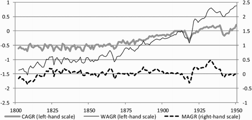
Figure 2. The logarithms of per capita demand of food products, wage deflated by food prices and non-food prices deflated by food prices, 1804–1950 (1913 = 0).

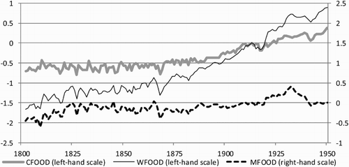
The series of agriculture and food display a similar development, although there is a larger rise over time in the demand for food products than for agricultural products, and likewise in the wage deflated by food prices than by agricultural prices. The deflated cross price was relatively stable during the investigated period, which suggests that various prices followed each other.

The wage deflated by agricultural or food prices reached a low point in the early nineteenth century. It was not until the second half of the nineteenth century that per capita demand and the deflated wage started to grow. Consumption of animal products increased its share in food demand. The sharpest declines in demand and real wage occurred due to the specific circumstances of the harvest failure in 1867 and the World Wars.

During the whole period of investigation Sweden was a net importer of agricultural and food products. r never reached a level above unity. As in UK (Clark, O’Rourke, & Taylor, 2014), over time Sweden even became more dependent on import of foodstuff.

4. Investigating cointegrating relationships

A complicating factor when applying the demand approach is the existence of endogeneity between the variables. For example, causations can go both ways. Estimating the true elasticities of demand may necessitate instrumentations. However, it is likely that the true elasticites fluctuated and changed through time. Knowing the true elasticities therefore does not necessarily yield an appropriate method to construct pre-industrial historical national accounts. The present study does not focus on the causal effects, but on evaluating methods of predicting agricultural and food demand back in time from series of prices and wages.

The method to estimate various coefficients from time series in order to predict per capita demand depends on the nature of these series. If they are stationary the absolute levels of the logarithms can be regressed. However, if they are not stationary other procedures should be used. If they are trend stationary the regression can include a time trend. If the series are stochastic and there is no cointegrating relationships the appropriate method is to regress first differences. If there is a common stochastic trend the variables can be modelled as cointegrated. The problem is that deciding on the nature of the time series is not always straightforward, and is sensitive to various assumptions and the chosen significance levels.

We start to investigate whether the various series are stationary, trend stationary or stochastic. The results concerning tests of unit root depends whether a trend is included or not. Here Table 1 displays the results, when a trend is included. The null of a unit root cannot be rejected for any of the series, except for non-agrarian prices (M_AGR), where the null is rejected in two out of three criteria for the chosen lag length and per capita consumption of agrarian products (C_AGR), where the null is rejected in one of the criterion used.

Table 1. DF-GLS tests of the existence of unit root for different series.

	Lag length selected using opt lag (Ng-Perron seq t)	Lag length selected using min SC	Lag length selected using MAIC
CAGR	9 lags: H0 not rejected	1 lag: H0 rejected at p = 5%	3 lags: H0 not rejected
WAGR	6 lags: H0 not rejected	1 lag: H0 not rejected	3 lags: H0 not rejected
MAGR	10 lags: H0 rejected at p = 5%	1 lag: H0 rejected at p = 1%	3 lags: H0 not rejected
CFOOD	6 lags: H0 not rejected	3 lags: H0 not rejected	9 lags: H0 not rejected
WFOOD	10 lags: H0 not rejected	1 lag: H0 not rejected	10 lags: H0 not rejected
MFOOD	10 lags: H0 not rejected	3 lags: H0 not rejected	3 lags: H0 not rejected

Notes: Based on trend. The null hypothesis assumes there is a unit root.

In practice it is difficult to distinguish between a series containing a unit root and a trend stationary series, especially if the trend is non-linear. One method to estimate the elasticities is to perform regressions, where the logarithm of per capita demand is the dependent variable, while the independent variables are detrended by including time variables. The demand approach must then be combined with other methods to determine changes in the trend for earlier periods, for example, studies on consumption patterns at some benchmark years. Then again, the main research purpose of this paper is to investigate to what extent the demand approach can also yield reasonable results for long-term trends, which is crucial if the approach is to be used for the construction of historical national accounts when no other indicators exists. This study therefore focuses on investing the cointegrating relationships.

To investigate common stochastic trends of the variables, cointegration tests are first performed on demand and the deflated wage, and subsequently also on the deflated cross price. The Johansen test is used. In contrast to the Engle-Granger procedure it does not rest on assuming that one of the variables are causally prior to the other (see Appendix 2 for details).

Testing for the appropriate number of lags, various criteria yield different results, and are sensitive to assumption of constants and trends. Appendix 2 provides the details. Based on that analysis, four different specifications of cointegration are analysed, two for agriculture and two for food. The result is summarised in Table 2. Two of the specifications only include demand and wage, while two of the specifications also include cross price. The specifications are also marked in bold in Table A1 in Appendix 2.

Table 2. Coefficients of the cointegration equations in four different specifications, 1804–1950.

	(1)	(2)	(3)	(4)
	Agriculture	Food	Agriculture	Food
Equation (1), ΔC the dependent variable
Cointegrating vector	−.257*** (.070)	−.287** (.109)	−.323*** (.068)	−.560*** (.121)
ΔCt−1		−.135 (.104)		−.025 (.097)
ΔWt−1		−.176^† (.101)		.396* (.181)
ΔMt−1				−.641*** (.174)
Constant			−.002 (.006)	.001 (.006)
R^2 (p > chi^2)	.0849 (.0002)	.1903 (.0000)	.1386 (.0000)	.3592 (.0000)
Equation (2), ΔW the dependent variable
Cointegrating vector	.065 (.082)	.117 (.110)	−.047 (.081)	−.008 (.125)
ΔCt−1		−.029 (.105)		.027 (.101)
ΔWt−1		.101 (.102)		.813*** (.188)
ΔMt−1				−.840*** (.181)
Constant			.014^† (.007)	.005 (.007)
R^2 (p > chi^2)	.0042 (.4418)	.0227 (.3438)	.0335 (.0824)	.1818 (.0000)
Equation (3), ΔM the dependent variable
Cointegrating vector			−.068 (.068)	−.062 (.129)
ΔCt−1				.064 (.104)
ΔWt−1				.567** (.193)
ΔMt−1				−.599** (.186)
Constant			−.001 (.006)	−.006 (.007)
R^2 (p > chi^2)			.0069 (.6048)	.0800 (.0314)
Cointegrating vector
C	1(default)	1(default)	1(default)	1(default)
W	−.376*** (.026)	−.423*** (.017)	−.270** (.086)	−.588*** (.042)
M			.082 (.135)	.338*** (.083)
Trend			−.002 (.001)	.002** (.001)
Constant	.150*** (.021)	.096*** (.016)	.284 (default)	−.128 (default)
p > chi^2	.0000	.0000	.0046	.0000
Observations	147	147	147	147

***Significant at a 0.1% level.

**Significant at a 1% level.

*Significant at a 5% level.

^†Significant at a 10% level.

In all the four specifications the coefficient of W in the cointegration vector are positive and significant. This entails that there is very likely a cointegration, and that we should not proceed towards regressing first differences.

Model (1) can be written as followed:(7)

The cointegration equation entails an elasticity of per capita demand for agricultural product with respect to deflated wage of 0.376, that is, an increase in wage by 1% tend to increase the demand in the long-term by 0.4%. Changing the period does not change the estimated elasticity to any large degree. An advantage to also include the last decades is that we then can take into account the impact of declining living standards during the two World Wars. The adjustment is, however, quite slow. It is demand that adjusts and not the wage. The speed-of-adjustment coefficient, a measure of how fast the equilibrium relation between the cointegrating variables is restored (see Appendix 2), for ΔC_AGR is −0.257, and significant. It entails that all else being equal, an increase in wage by 1% above equilibrium tend to increase the per capita demand of agricultural products by 0.1% (−0.257 times −0.376) during the first year. The speed-of-adjustment parameter for ΔW_AGR is not significantly different from zero, but of the right sign (i.e. positive), which may suggest that wage is weakly exogenous.

Model (1) encompasses C_FOOD and W_FOOD. The lags of differences are also included on the right-hand side of the equation. The cointegrating vector and the speed-of-adjustment coefficients have almost the same values as in Model (1). None of the lags are significant at a 5% level, although the coefficient of ΔW_{FOOD ,t−1} in Equation (1) is significant at a 10% level.

In Models (3) and (4) the cross price is also included. The most important aspect is that the coefficient of M_t−1 in the cointegrating vector is positive in both models, and of opposite sign of the coefficient of W_t−1. The coefficient of M_FOOD ,_t−1, at +0.338, is strongly positive, entailing a negative cross price elasticity of demand. This suggests that there are no strong empirical reasons to assume a positive cross price elasticity of demand. Furthermore, since a trend is included, these two models are not as relevant to predict changes in long-term trends.

5. Reliability checks

Out-of-sample estimation may serve as a reliability check. To perform out-of-sampling only the specification of the cointegrating vector of Model (1) and Equation (7) is used to predict per capita demand of agricultural products. The cointegrating vector describes the equilibrium condition, which is what is calculated. When there is no deviation from this equilibrium condition, there is no adjustment process. If further lags are included there could be further movements, but the Model (1) does not include any more lags. Figure 3 presents the prediction for the first and last 50 years. For the period 1852–1950, the cointegrating relationship is C_AGR = −0.11 + 0.35W_AGR, which is used to predict demand in 1802–1851, while for the period 1803–1900 the cointegrating relationship is C_AGR = −0.12 + 0.41W_AGR, which is used to predict the demand in 1901–1950.

Figure 3. Per capita consumption of agricultural products in Sweden, predicted (1365–1830) and actual (1802–1950) 1913 = 100. Source: See Appendix 1.

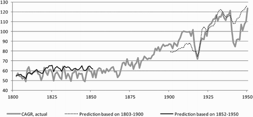
For the period 1802–1851 the root mean square error (RMSE) is calculated to 0.10 natural logarithms and for the period 1901–1950 to 0.11 natural logarithms. The root median square error is smaller, only 0.07 natural logarithms for the period 1802–1851 and 0.08 natural logarithms for the period 1901–1950. It should be considered that the series of agricultural demand estimated from official statistics, although being unbiased, also deviates from the true levels of agricultural demand. This further increases the uncertainty of how reliable the demand approach is. Term the first root means square error as RMSE_DA and the second as RMSE_HNS, while RSME is the root mean square error of the demand approach from the estimate of the historical national accounts that we have been able to calculate. Let a be the error of the historical national accounts relative the error of demand approach (i.e. RMSE_HNS/RMSE_DA), and ρ be the correlation between the two errors. After some rewriting we have:(8)

While a larger error of the historical national accounts compared to the demand approach, that is, a higher a, decreases RMSE_DA compared to RMSE, a higher ρ have the opposite effect. Since we do not know if a² is larger or smaller than 2aρ, we do not know whether RMSE_DA is larger or smaller than RMSE. However, it is likely that the difference is not so large. For example, assume that the RMSE of the historical national accounts series was 50% of the RMSE of the demand approach in 1802–1851 and ρ was 0.25 – quite plausible assumptions. Then the RMSE_DA equals the RMSE for that period. For later periods a should be smaller, but so should also ρ.

Assuming RMSE_DA is close to RMSE, the 90% confidence interval of the estimate of the demand approach should be ±0.16 and ±0.20 natural logarithms, respectively. It can be compared to the grading scale, from A to D, suggested by Feinstein (1972, pp. 20–22) for historical national accounts. He terms grade B a ‘good estimate’, which has a 90% subjective margin of error of ±5–15%. He calls grade C a ‘rough estimate’, which has a per cent subjective margin of error ±15–25%. The prediction resulting from the demand approach yields estimates that according to Feinstein’s terminology is ‘rough’. The fit is far from being perfect, and there are some important deviations. A worrying sign is that some of the annual fluctuations may be underestimated. Since the average error is larger than the median error, we may suspect that the demand approach could produce large errors for some individual years or periods. However, interestingly the deviations after some time seem to return to the estimated equilibrium.

Figure 3 shows that the predictions yield reasonable results. While the prediction displays an increase in per capita demand in the first decades of the nineteenth century, the estimate of historical national accounts declined. An explanation for the lower levels of agricultural demand in the 1830s and 1840s compared to the first decade of the nineteenth century was the expansion of the potato, which allowed a lower per capita volume demand, even if the production of per capita animal products bottomed out around 1800 (Gadd, 2011, p. 145). Such one-off innovation is difficult to model correctly.

The rise in per capita demand in the early twentieth century is underestimated by the prediction in Figure 3. Around 1900 consumption patterns changed dramatically. The consumption of grains and potatoes stagnated, while the consumption of sugar, fats and pork expanded (Morell, 2011, pp. 188–189). For this period the linear model may underestimate the elasticity of agricultural demand.

While the decline in per capita demand during the First World War is well predicted in Figure 3, this is not the case for the sharp decline in per capita demand in the early 1940s. The decline in the early 1940s was due to the particular circumstances of the outbreak of the Second World War. The war affected all branches, not least agriculture, which were dependent on imported supplies (Johansson, 1985, pp. 182–196; Morell, 2001, pp. 182–186). Prices were regulated. From 1940 all basic food products, except potatoes and milk, were rationed. During these years the relation between price and demand was therefore distorted compared to a free market situation. By 1950, the level according to historical national accounts had almost returned to the predicted equilibrium level.

Another reliability check of the demand approach is to use the estimated parameters derived for 1802–1950 to back project the consumption of agrarian products in Sweden. We then use a wage series that goes back to 1365, which is deflated by a price index of agrarian products (see Appendix 1). A problem is that the number of days worked during the year has changed over time. Here an adjustment is made based on the number of holidays, which has been reduced since the Middle Ages following the Reformation. Given that the data on wages have a lower representativity before 1732, we should expect an even wider 90% confidence interval than the one estimated from out-of-sampling.

Previous studies on historical national accounts also present data on the development of agriculture before the nineteenth century. Schön and Krantz (2012) use the demand approach, while Edvinsson (2013b) follows earlier studies on living conditions in assuming a constant consumption pattern in the eighteenth century. However, these data are not comparable to the series of agricultural demand presented here. Instead this study directly compares the demand approach based on actually derived elasticities with earlier studies on consumption patterns and heights.

Figure 4 presents the estimates using the demand approach and the derived cointegration Equation (7). Previous research in Sweden has concluded that food consumption worsened from the sixteenth to the seventeenth century (Morell, 1987), although there are some uncertainties concerning various weight and volume measures, and the representativity of the underlying material. The estimates from the demand approach instead suggest that the deterioration was not so great between those two centuries, although there was a decline between the sixteenth and eighteenth centuries. Figure 4 points towards a sharp deterioration in the early sixteenth century, during the course of just one generation. Between the fifteenth and sixteenth centuries, the median level decreased by 23%. Agricultural consumption in the fifteenth century was according to the estimates of Figure 4 very high, at a level not surpassed until the 1890s. How does this accord with earlier research and other indicators?

Figure 4. Actual level of the logarithm of per capita agricultural demand, and out-of-sample predictions for the first and last 50 years in 1802–1950 based on the cointegration relationship of demand and wage.

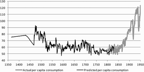
An important indicator of living standards is human height (Öberg, 2014). More animal products in the diet increase the ability of the body to absorb key vitamins and minerals, which in turn improves physiological structure (Logan, 2006, p. 540). The long-term trends in human heights very roughly mirror the picture in Figure 4, that is, good conditions in the Middle Ages, worsening conditions in the eighteenth and early nineteenth centuries and an improvement from the mid-nineteenth century onwards. Earlier studies on Sweden shows that the average height of soldiers did not change between the eighteenth and early nineteenth centuries (Gustafsson, Werdelin, Tullberg, & Lindenfors, 2007, p. 862), staying at between 166 and 168 cm. These sources are reliable, but there are some uncertainty concerning to what extent average heights of soldier’s corresponded to the average heights of males. An archeologic finding for the seventeenth century puts the average height of men at 169.6  cm (Gustafsson et al., 2007, p. 870). In the late Middle Ages, archeologic findings exhibit average heights for men of between 170 and 174 cm (partly reflecting regional differences), which is equivalent to the average heights measured for men born in the 1890s (Öberg, 2014, p. 17), levels that mirrors surprisingly well Figure 4.

We can also compare the result from Figure 4 with studies on consumption patterns. For simplicity, we here assume that the calorie intake per person did not change in the long-term in accordance with the constant calorie approach (Kaneda, 1968, p. 5), and that the volume of per capita food consumption only shifted with changed composition. Before the twentieth century, the calorie intake was at a high level due to hard work, and could not be assumed to be below even present levels.

According to Morell (1987, p. 103), between the sixteenth and eighteenth centuries, among agricultural labourers, the proportion of calories coming from animal products decreased from 25.7% to 13.9% and coming from beer from 15.9% to 6.4%. Assuming that one calorie consumed from animal products increased the per capita volume 4–6 times compared to one calorie consumed from bread, while beer increased the volume 2–2.5 times, entails that the per capita consumption of agrarian products was about 30–40% higher in the sixteenth century than in the eighteenth century. In contrast, the estimate in Figure 4 puts the median level in the sixteenth century only 13% higher. The true level may have been in between those two estimates, which would entail that the result from the demand approach is within the confidence interval of ±20–30%. In contrast, Figure 4 put the median consumption level in the fifteenth century at 47% higher level than in the eighteenth century. A study by Söderberg (2014) on the composition of food consumption in the late Middle Ages shows that the consumption of beer and animal products may indeed have been higher than in the sixteenth century.

Another deviation in Figure 4 from what we know from earlier research is the high estimated levels in the early eighteenth century. The median level in Figure 4 in 1690–1730 was 15% above the median level in the rest of the eighteenth century. In contrast, recruited soldiers that were born in the 1720s were shorter than men in any other period for which there is data. The calorie intake in Swedish ‘hospitals’ was much lower in the period 1690–1730 than in other periods, but stabilised from the 1740s at a higher level (Morell, 1989). To this background, it is likely that the demand approach for this period produces results at the top of a possible ±20–30% confidence interval.

6. Conclusions

This study presents some empirical evidence from the Swedish data that the demand approach, with some caveats, could be used to reconstruct pre-industrial national accounts, but the estimates will at best be rough. A more rigorous time series analysis, including tests of stationarity and (if the variables contain a stochastic trend) cointegration, is necessary, which presupposes reliable annual data for a longer period. The main contribution to the field is that the demand approach is operationalised as a cointegrating relationship, that the agricultural data underpinning this study for the early nineteenth century is more reliable than for other countries and by estimating the margin of error using the approach. This study reformulates the demand approach, by studying the relation between demand and the deflated wage and cross price, where the deflator used is the agrarian or food price. Instead of transferring parameters from other studies, this study also applies the estimated cointegaring relationship to back-project consumption of agricultural products in Sweden back to the Middle Ages.

Since this study finds no strong empirical evidence that the cross price elasticity of demand is positive, the demand approach could be simplified into only using coefficients of the wage deflated by agricultural or food prices. It simplifies the task to collect data in order to apply the demand approach and interpreting the cointegrating relationship.

A problem with the demand approach is that daily wage is not a very reliable indicator of incomes, especially if it only covers a smaller segment of male labour. The present study uses a series of annual incomes back to 1850, while the series of daily wage could be a good indicator of the movements in annual income in the first half of the nineteenth century. There is no evidence of a shift in worked days per year in the first half of the nineteenth century. However, during the early modern period, the industrious revolution must be taken into accounts when applying the demand approach. In this period annual wage probably developed less negatively than daily wage, due to an increase in days worked per year. Adjustments are therefore made to the series of daily wage by taking account of changes in the number of holidays.

Does the demand approach advance our knowledge of the pre-industrial economies? The food puzzle in the British economy between 1770 and 1850 exemplifies why the approach may not yield any reliable results at all (Clark et al., 1995). When no other indicators exist on long-term trends, the present study suggests that the demand approach can yield reasonably rough estimates of agricultural consumption and production. For Sweden, income elasticity is estimated to around +0.4, which is robust to the model applied and in line with earlier international research. Assuming the cross price elasticity was zero, this would entail that price elasticity was −0.4.

Out-of-sampling shows that reasonable predictions can be attained from the demand approach. If the underlying data is reliable we can expect a 90% confidence interval of ±15 to ±25%. However, such large confidence intervals should make us aware of not assuming too much from the data generated by the demand approach, especially if the estimated levels contradict other more direct sources. Previous research has hitherto refrained from using the series derived from the demand approach for econometric analysis, which is wise. When back-projecting it would be preferable to combine the demand approach with other indicators of agricultural and food consumption, both for estimating long-run trends and short-term deviations from these trends. In this study a comparison is made with two other indicators: data on heights and direct sources on the composition of food consumption. All three indicators points towards a decline in per capita food consumption from the late Middle Ages to the eighteenth century. The level in the late Middle Ages as compared to the late nineteenth century according to the demand approach is congruent with the development of human heights. For the Middle Ages the demand approach improves our knowledge of the pre-industrial economy compared to using, for example, the constant per capita consumption approach (Dean & Cole, 1962; Grytten, 2003). However, for the sixteenth century the demand approach may underestimate the actual level in Sweden. For the early eighteenth century it may overestimate the actual Swedish level, a result even inferior to the constant per capita consumption approach. However, such occasional ‘food puzzles’ are to be expected for cointegrated variables if the speed-of-adjustment is slow and if there are medium-term oscillations in the equilibrium relations. The demand approach should therefore preferably be used in combination with other empirical indicators of agricultural consumption.

Disclosure statement

No potential conflict of interest was reported by the author.

Additional information

Funding

The author greatly acknowledges financial support from Riksbankens Jubileumsfond; Swedish Collegium for Advanced Study; Vetenskapsrådet; and Jan Wallanders och Tom Hedelius Stiftelse.

Appendix 1. The data

The series of agricultural and food production after 1802 is explained in earlier studies (Edvinsson, 2013a, 2013b, 2014). In Swedish historical national accounts direct annual data on harvests exists from 1802. Harvests are recorded for the harvest year. Both published and unpublished official sources are used. It is the agricultural output that is investigated and not the value added, since intermediate consumption is not deducted. However, agricultural output is deducted of intermediate consumption coming from agriculture, such as seeds, forage and milk used by calves, as is common in national accounts. Agriculture here includes items not used as food, for example, the production of linen and wool, but excludes forestry.

Direct annual data on animal production (derived from the annual data on the animal stock) can only be calculated from around 1870. For the period before, annual fluctuations in the animal produce are estimated from the lagged fluctuations in the supply of grains. Food industries are similarly derived from the movements in the supply from agriculture.

Food production includes the whole output of food industries. It also includes the part of agricultural output that was consumed directly and not used as intermediate consumption in food industries, mainly, potatoes, peas, milk, fish and horticulture.

Demand is estimated as production plus import less export. The import and export series are from official data and earlier research (Åmark, 1915; Johansson, 1967; Schön & Krantz, 2012; Statistics Sweden, 1972). For simplicity the same price index is used for demand as for output (otherwise, some of the assumptions made in the demand approach must be modified).

Prices from 1802 onwards are from historical national accounts (Edvinsson, 2005, 2014). Agrarian prices are from the end-of-year. Current year’s grain prices, therefore, corresponds with current year’s harvest. The price index of agriculture is the same as the price index of the output of agriculture (including fisheries, but excluding forestry). The non-agrarian and non-food prices are the same, and consists of the Fisher price index of textile and leather industries (100% of output included), stone and clay industries (30%), wood industries (10%), paper industries (10%), chemical industries (10%), engineering (10%), power, gas and waterworks (50%), railways (50%), car transports (70%), sea transports (10%), air transports (50%), animal transports (20%), postal services (20%), telecommunications (30%), hotels and restaurants (100%), housing (100%), paid domestic services (100%) and other private services (100%). The proportions of the outputs included in the price index are roughly derived from assumptions made in Swedish historical national accounts concerning the distribution of output to different uses (Edvinsson, 2005; Schön & Krantz, 2012).

Nominal wage is from 1850s onwards the average annual wage among wage-earners according to Swedish historical national accounts (Edvinsson, 2005). The reliability of the data is lower before 1913 (Bengtsson, 2014). To extrapolate this series backwards, an unweighted geometric average of the daily wage of a male labourer without horses and a male labourer with two horses is used (Jörberg, 1972). The agricultural wage was reported late in the year, so the current year’s wage rate was also used in the subsequent year. It may be assumed that days worked per year did not change in the period 1802–1850, and that a possible industrious revolution took place before 1802.

For the period 1732–1802, the wage series is based on the same source as for the period 1802–1850 (Jörberg, 1972). For the period before 1732, there exist only a series of day workers in Stockholm, with data as far back as 1365 (Söderberg, 2010). The assumption is that the number of days worked was 265 up to 1530, increased linearly to 285 up to 1600, decreased linearly to 283 up to 1620, stayed at 283 up to 1700, increased linearly to 285 up to 1720, stayed at 285 up to 1772 and increased linearly to 300 up to 1802 (Myrdal, 1999, pp. 305–308). Prices for 1732–1802 are based on Jörberg (1972), and before 1732 on the material underpinning the study of Edvinsson and Söderberg (2011).

Appendix 2. Details on the cointegration model

In the Johansen’s test, the specific model in its simplest n-variable form can be written as:(A1) is the vector of the n variables at time t, an vector of constants, an vector of errors and an n · n matrix. If there is cointegration, the matrix can also be written as , where both and are n · r vectors and r is the rank of matrix . The rank of matrix is equivalent to the number of non-zero eigenvalues or the number of cointegration vectors. If the rank of the matrix is zero, it entails that no cointegration relations exists, while if there is full rank (i.e. if r = n) the vector process is stationary. Adding lags, constants and trends, Equation (A1) can be written as a vector-error correction model (where p is the number of lags, and are vectors, and are vectors, and are n · n matrices):(A2)

With only one lag the expression is deleted from the equation. The coefficents of are generally interpreted as the speed-of-adjustment coefficients, while is the cointegrating vector. and expand the cointegrating vector. One of the coefficients of is usually normalised to 1 by default, which also yields specific coefficients of .

Hannan–Quinn information criterion (HQIC) and Schwarz Bayesian information criterion (SBIC) provide the most consistent estimates of the true lag length (Lütkepohl, 2005). However, both for agriculture and food, when only a constant is included in the cointegrating vector, HQIC and SCIC suggest different lags (see Table A1). The chosen models have been decided on whether any of the last lags are significant or not.

Table A1. Test of lag length of the vector-error correction model.

Variables included in the VEC model	No constant, HQIC	No constant, SBIC	Constant included, HQIC	Constant included, SBIC
CAGR, WAGR	2	2	2	1
CFOOD, WFOOD	2	2	3	2
CAGR, WAGR, MAGR	2	2	1	1
CFOOD, WFOOD, MFOOD	2	2	2	1

Table A2 displays the results of the Johansen’s test of the cointegrating rank of a vector-error correction model. The result depends on whether constants and trends are included. λ_trace statistics are calculated, where the number of non-zero eigenvalues are tested. In the first test, the null hypothesis is that r = 0, and the alternative hypothesis is that r > 0. In the second test, the null hypothesis is that r ≤ 1 and the alternative hypothesis that r > 1. In the third test (for the three-variable case), the null hypothesis is that r ≤ 2 and the alternative hypothesis that r > 2.

Table A2. Test of cointegration rank of the vector-error correction model depending on specification.

Variables included	Lags	Unrestric­ted trend	Restricted trend	Unrestric­ted constant	Restricted constant	No trend
CAGR, WAGR	1	r > 1	r > 0 r ≤ 1	r > 0 r ≤ 1	r > 0 r ≤ 1	r = 0
	2	r > 1	r > 0 r ≤ 1	r = 0	r = 0	r = 0
CFOOD, WFOOD	2	r > 1	r > 0 r ≤ 1	r > 0 r ≤ 1	r > 0 r ≤ 1	r > 0 r ≤ 1
	3	r > 0 r ≤ 1	r = 0	r > 0 r ≤ 1	r > 0 r ≤ 1	r > 0 r ≤ 1
CAGR, WAGR, MAGR	1	r > 0 r ≤ 1	r > 0 r ≤ 1	r > 2	r > 2	r > 0 r ≤ 1
	2	r = 0	r = 0	r > 2	r > 2	r > 1 r ≤ 2
CFOOD, WFOOD, MFOOD	1	r > 1 r ≤ 2	r > 1 r ≤ 2	r = 0	r = 0	r > 1 r ≤ 2
	2	r > 0 r ≤ 1	r > 0 r ≤ 1	r > 1 r ≤ 2	r = 0	r > 1 r ≤ 2

Four alternative combinations of variables are investigated, including and excluding cross price, for agriculture and food, respectively. This is done for various lag lengths. In addition, five different specifications are made concerning the inclusion of constants and trends. A problem when testing the rank of matrix is that the result is sensitive to these specifications.

If the purposes of the demand approach is to determine the movements in the trend itself, no trend should be included in the specification, except for a constant in the cointegrating vector. If a time trend is included, we cannot assume that the coefficients for the constants or trends are the same for earlier periods. The demand approach must then be combined with other estimates concerning long-term trends at some benchmark periods.

No specification is chosen with no constant in the cointegrating vector. Such a constant is necessary to include given that the logarithms are set to zero for the year 1913 (and this choice is arbitrary). With C_AGR, W_AGR and a restricted constant only one lag works, since including two lags entails that there is no cointegration. With C_FOOD, W_FOOD and a restricted constant the choice falls on two lags in the specification, since none of the last lags are significant in a specification with three lags.

With three variables, none of the models works that only include a restricted constant, since such specifications would entail zero or full rank of matrix . These models are more difficult to interpret. The choice falls on specification with a restricted trend, and only one cointegrating vector. If there are more than one cointegrating vector the interpretation is not straightforward, since then any linear combination of these vectors is also a cointegrating vector.

References

- Allen, R. (2000). Economic structure and agricultural productivity in Europe, 1300–1800. European Review of Economic History, 4, 1–25. doi: 10.1017/S1361491600000125
- Allen, R. (2005). English and Welsh agriculture, 1300–1850: Output, inputs, and income. Unpublished manuscript.
- Álvarez-Nogal, C., & Prados de la Escosura, L. (2007). The decline of Spain (1500–1850): Conjectural estimates. European Review of Economic History, 11, 319–366. doi: 10.1017/S1361491607002043
- Álvarez-Nogal, C., & Prados de la Escosura, L. (2013). The rise and fall of Spain (1270–1850). The Economic History Review, 66, 1–37. doi: 10.1111/j.1468-0289.2012.00656.x
- Álvarez-Nogal, C., Prados de la Escosura, L., & Santiago-Caballero, C. (2015). Agriculture in Europes little divergence. The case of Spain. EHES Working Papers in Economic History, no. 80.
- Åmark, K. (1915). Spannmålshandel och spannmålspolitik i Sverige 1719–1830. Stockholm: Stockholms högskola.
- Arroyo Abad, L., & van Zanden, J. L. (2014). Growth under extractive institutions? Latin American per capita GDP in colonial times. CGEH Working Paper Series, Middlebury College, no. 61.
- Bassino, J.-P., Broadberry, S., Fukao, K., Gupta, B., & Takashima, M. (2015). Japan and the great divergence, 725–1874. CEPR Discussion Paper Series, no. 10569.
- Bengtsson, E. (2014). Labours share in twentieth-century Sweden: A reinterpretation. Scandinavian Economic History Review, 62, 290–314. doi: 10.1080/03585522.2014.932837
- Berg, B.-Å. (2007). Volatility, integration and the grain banks: Studies in harvests, rye prices and institutional development of Parish Magasins in Sweden in the 18th and 19th centuries. Stockholm: Stockholm School of Economics.
- Broadberry, S., Campbell, B., Klein, A., Overton, M., & van Leeuwen, B. (2010). British economic growth, 1270–1870. London: London School of Economics. Unpublished manuscript.
- Broadberry, S., Custodis, J., & Gupta, B. (2015). India and the great divergence: An Anglo-Indian comparison of GDP per capita, 1600–1871. Explorations in Economic History, 55, 58–75. doi: 10.1016/j.eeh.2014.04.003
- Broadberry, S., Guan, H., & Li, D. D. (2012). China, Europe and the great divergence: A study in historical national accounting. Unpublished manuscript.
- Clark, G. (2010). The macroeconomic aggregates for England, 1209–2008. Research in Economic History, 27, 51–140. doi: 10.1108/S0363-3268(2010)0000027004
- Clark, G., Huberman, M., & Lindert, P. H. (1995). A British food puzzle, 1770–1850. Economic History Review, 48, 215–237.
- Clark, G., O’Rourke, K., & Taylor, A. (2014). The growing dependence of Britain on trade during the industrial revolution. Scandinavian Economic History Review, 62, 109–136. doi: 10.1080/03585522.2014.896285
- Crafts, N. F. R. (1976). English economic growth in the eighteenth century: A re-examination of Deane and Cole’s estimates. The Economic History Review, 29, 226–235. doi: 10.2307/2594312
- Crafts, N. F. R. (1980). Income elasticities of demand and the release of labour by agriculture during the British industrial revolution. Journal of European Economic History, 9, 153–168.
- Crafts, N. F. R. (1985). British economic growth during the industrial revolution. Oxford: Clarendon Press.
- Dean, P., & Cole, W. A. (1962). British economic growth, 1688–1959: Trends and structure. Cambridge: Cambridge University Press.
- Edvinsson, R. (2005). Growth, accumulation, crisis: With new macroeconomic data for Sweden 1800–2000. Stockholm: Almqvist & Wiksell.
- Edvinsson, R. (2009). Swedish harvests 1665–1820: Early modern growth in the periphery of European economy. Scandinavian Economic History Review, 57, 2–25. doi: 10.1080/03585520802631592
- Edvinsson, R. (2013a). Swedish GDP 1620–1800: Stagnation or Growth? Cliometrica, 7, 37–60. doi: 10.1007/s11698-012-0082-y
- Edvinsson, R. (2013b). New annual estimates of Swedish GDP in 1800–2010. The Economic History Review, 66, 1101–1126.
- Edvinsson, R. (2014). The gross domestic product of Sweden within present borders 1620–2012. In R. Edvinsson, T. Jacobson, & D. Waldenström (Eds.), Historical monetary and financial statistics for Sweden, Volume II: House prices, stock returns, national accounts, and the Riksbank balance sheet, 1620–2012 (pp. 101–182). Stockholm: Sveriges Riksbank and Ekerlids.
- Edvinsson, R., & Söderberg, J. (2011). A consumer price index for Sweden 1290–2008. Review of Income and Wealth, 57, 270–292. doi: 10.1111/j.1475-4991.2010.00381.x
- Feinstein, C. (1972). National income, expenditure and output of the United Kingdom 1855–1965. Cambridge: Cambridge University Press.
- Gadd, C.-J. (2011). The agricultural revolution in Sweden, 1700–1870. In M. Morell & J. Myrdal (Eds.), The agrarian history of Sweden: 4000 BC to AD 2000 (pp. 118–164). Lund: Nordic Academic Press.
- Grytten, O. (2003). Output, input and value added in Norwegian agriculture, 1830–1865. In G. Jonsson (Ed.), Nordic historical national accounts: Proceedings of workshop VI Reykjavik 19–20 September 2003 (pp. 47–76). Reykjavik: Institute of History, University of Iceland.
- Gustafsson, A., Werdelin, L., Tullberg, B., & Lindenfors, P. (2007). Stature and sexual stature dimorphism in Sweden, from the 10th to the end of the 20th century. American Journal of Human Biology, 19, 861–870. doi: 10.1002/ajhb.20657
- Humphries, J., & Weisdorf, J. (2014). The wages of women in England, 1260–1850. Retrieved from http://jacobweisdorf.files.wordpress.com/2012/04/womens-wages_humphries-and-weisdorf_feb-20143.pdf
- Jackson, R. V. (1985). Growth and deceleration in English agriculture, 1660–1790. The Economic History Review, XXXVIII, 333–351.
- Johansson, M. (1985). Svensk industri 1930–1950: Produktion, produktivitet, sysselsättning. Lund: Studentlitteratur.
- Johansson, Ö. (1967). The gross domestic product of Sweden and its composition 1861–1955. Stockholm: Almqvist & Wiksell.
- Jörberg, L. (1972). A History of Prices in Sweden 1732–1914. Lund: Gleerup.
- Kaneda, H. (1968). Long-term changes in food consumption patterns in Japan, 1878–1964. Food Research Institute Studies, 8, 3–32.
- Logan, T. (2006). Food, nutrition, and substitution in the late nineteenth century. Explorations in Economic History, 43, 527–545. doi: 10.1016/j.eeh.2005.07.002
- Lütkepohl, H. (2005). New introduction to multiple time series analysis. Oxford: Springer.
- Maddison, A. (2010). Historical statistics of the world economy: 1–2008 AD. Retrieved from http://www.ggdc.net/maddison/Historical_Statistics/horizontal-file_02-2010.xls.
- Malanima, P. (2011). The long decline of a leading economy: GDP in central and northern Italy, 1300–1913. European Review of Economic History, 15, 169–219. doi: 10.1017/S136149161000016X
- Molinas, C., & Prados de la Escosura, L. (1989). Was Spain different? Spanish historical backwardness revisited. Explorations in Economic History, 26, 385–402. doi: 10.1016/0014-4983(89)90015-6
- Morell, M. (1987). Eli F. Heckscher, the ‘food budgets’, and Swedish food consumption from the 16th to the 19th century. Scandinavian Economic History Review, 35, 67–107. doi: 10.1080/03585522.1987.10408082
- Morell, M. (1989). Studier i den svenska livsmedelskonsumtionens historia: hospitalhjonens livsmedelskonsumtion 1621–1872. Uppsala: Uppsala University.
- Morell, M. (2001). Jordbruket i industrisamhället. Lagersberg: Natur och Kultur & LTs Förlag.
- Morell, M. (2011). Agriculture in industrial society, 1870–1945. In M. Morell & J. Myrdal (Eds.), The agrarian history of Sweden: 4000 BC to AD 2000 (pp. 165–213). Lund: Nordic Academic Press.
- Myrdal, J. (1999). Jordbruket under feodalismen 1000–1700. Stockholm: Natur och kultur & LT.
- Nielsen, R. (1997). Storage and English Government intervention in early modern grain markets. The Journal of Economic History, 57, 1–33. doi: 10.1017/S0022050700017903
- Öberg, S. (2014). Social bodies: Family and community level influences on height and weight, southern Sweden 1818–1968. Gothenburg: University of Gothenburg.
- Persson, K.-G. (2010). An economic history of Europe: Knowledge, institutions and growth, 600 to the present. Cambridge: Cambridge University Press.
- Pfister, U. (2011). Economic growth in Germany, 1500–1850. Unpublished manuscript.
- Schön, L., & Krantz, O. (2012). The Swedish economy in the early modern period: Constructing historical national accounts. European Review of Economic History, 16, 529–549. doi: 10.1093/ereh/hes015
- Söderberg, J. (2010). Long-term trends in real wages of labourers. In R. Edvinsson, T. Jacobson, & D. Waldenström (Eds.), Historical monetary and financial statistics for Sweden, Volume I: Exchange rates, prices, and wages, 1277–2008 (pp. 453–478). Stockholm: Sveriges Riksbank and Ekerlids.
- Söderberg, J. (2014). Oceanic thirst? Food consumption in mediaeval Sweden. Scandinavian Economic History Review, 63, 135–153. doi: 10.1080/03585522.2014.987315
- Statistics Sweden. (1972). Historisk statistik för Sverige. D. 3, Utrikeshandel 1732–1970. Stockholm: Author.
- Turner, M. E., Beckett, J. V., & Afton, B. (2001). Farm production in England 1700–1914. Oxford: Oxford University Press.
- Wrigley, E. A. (1967). A simple model of London’s importance in changing English society and economy 1650–1750. Past and Present, 37, 44–70. doi: 10.1093/past/37.1.44
- van Zanden, J. L., & van Leeuwen, B. (2012). Persistent but not consistent: The growth of national income in Holland 1347–1807. Explorations in Economic History, 49, 119–130. doi: 10.1016/j.eeh.2011.11.002