Labour and the ‘law of one price’: regional wage convergence of farm workers in Sweden, 1757–1980

ABSTRACT

Economic theory predicts that differences in wages for workers with similar skills will decline as labour mobility increase. This prediction is reminiscent of the ‘law of one price’, the notion that markets, if unfettered, eliminates price differentials of similar commodities across space. But can we really apply the economic logic of the commodity market to the labour market, governed as it is by institutions and politics as well as market forces? In this paper, we have examined the spread in farm workers’ wages across Swedish counties in 1757–1980. Besides nominal wages, the paper also offers cost of living indices by county. The paper enquires into sigma convergence and beta convergence. Long-run convergence, by both measures, was massive; the coefficient of variation, for instance, declined from about 28 per cent in the mid-eighteenth century to 4 per cent in 1980. Most of the compression, though, occurred in brief episodes rather than continuously. Markets, through labour mobility and trade, and institutions, through collective actions and labour laws, took turns in pushing towards regional convergence. The ‘law of one price’, we conclude, was not singlehandedly responsible for the elimination of regional wage differentials.

KEYWORDS:

• Law of one price
• regional wage convergence
• farm workers
• labour market institutions
• Sweden

JEL CODES:

• N33
• N34
• N93
• N94
• R12

1. Introduction

Mainstream economic theory forecasts that workers that have the same skills will receive equal payments in a fully integrated labour market (Marshall, 1920, book 6, Ch. 3; Hicks, 1932, Ch. 4). This prediction of equalisation in pay differentials is reminiscent of the so-called ‘law of one price’, a metaphor frequently used in research on convergence in commodity prices (Federico, 2012). Studies on price convergence suggest that the law applies so long as information flows freely between market actors and trade costs do not put wedges into price levels across separate locations (Cournot, [1838] 1971). A frequently used illustration of price convergence is when wheat began to be shipped large scaled from Chicago to Liverpool during the latter half of the nineteenth century, which implied that price differentials of similar wheat qualities had almost vanished by the early twentieth century (Harley, 1980; O’Rourke & Williamson, 1999). In a labour market context, the ‘law of one price’ would entail that wages across workers and locations would converge as transports and communication technologies increase labour mobility. But is it feasible to assume that the logic of the commodity market also applies to people, who do not only respond to incentives such as monetary gains?

In empirical terms, the prediction of wage convergence following the ‘law of one price’ should be supported by the elimination of wages differentials for similar workers across space.¹ Yet studies that look into the regional labour markets of the past have seldom found fully equalised wages, probably because workers have not met the mobility criterion, which in turn indicates that the necessary requirements for labour mobility were not satisfied.² Few studies stretch across wide time spans, but they provide evidence that regional wages seem to have converged since pre-industrial times, for the distribution of wages across space in the late twentieth and the early twenty-first century is rather flat (Collin, Lundh, & Prado, 2019). One explanation for the convergence of regional wages is likely to be found in radical improvements in transports and communications that took place in the latter half of the nineteenth century and hence favoured labour mobility.

The market forces commonly associated with the ‘law of one price’ are not the only possible reason for wage compression. Collective actions by workers and employers weaken the forces of the market. Labour unions and employers’ associations often decide the terms and conditions of employment and wages in collective agreements, ironing out market-induced wage differentials owing to skills and other labour characteristics. If wage differentials have decreased because collective agreements established a narrow range within which wages could vary, then convergence cannot be attributed to the ‘law of one price’. Hence, in a labour market context, the attribution of wage convergence to the ‘law of one price’ is not a semantic issue, it carries also an interpretation of the mechanism by which wage convergence is reached.

In order to examine when and where there has been a labour market transition from separation to integration, and what general mechanism that could possibly have caused it – unfettered markets or labour market institutions – we must have regional wage series that are homogeneous with regard to geographical coverage and labour characteristics. In addition, the wage series must also capture a wide time span, otherwise one might detect only brief spells of a convergence process subject to recurrent swings and temporary setbacks. Barring a recent study of manufacturing workers (Collin et al., 2019), researchers have thus far relied on regional wage series that span over half a century at most. As a result of the short time frames of previous studies, our knowledge about the long-term behaviour of regional wages is scanty.

This paper aims to fill the lacuna of long-term studies of regional wage convergence by looking into data for Sweden. We measure regional wage differences by examining data for farm workers in Sweden from a very long-term historical perspective, relying on homogenous wages series for 24 Swedish counties. The sources at our disposal provide an opportunity to establish a set of series beginning in 1757 and ending in 1980. We gathered regional wage series from various publications up to 1945, when the printed tables on county wages of agrarian workers ceased to be published. We extended the data with recourse to the original returns of the official wage statistics in 1950, 1955, 1960, 1970, and 1980. In addition to the prolonged record of nominal farm wages by county, the paper also offers new cost-of-living indices that span the 1757–1980 period in order to account for the potential influence that cost differentials might have had on nominal wage convergence. We want to remove all suspicion that nominal wage convergence is merely the corollary of convergence in cost differentials.

Our analytical strategy adheres to a practice common in convergence studies, enquiring into the spread of wage levels over time, the so-called σ-convergence, and into the tendency of low-wage counties to catch up with high-wage counties, the so-called β-convergence (Barro & Sala-i-Martin, 1991). Both testify to a real wage convergence across the entire period, manifested most significantly through a drop of the coefficient of variation from 28 to 4 percent. The rate of convergence varied over time, however, and convergence took place mostly in brief episodes, rather than continuously. Besides employing the cross-sectional approach, we also illustrate the panel-data design to estimate β-convergence using annual wages from 1757 to 1945 and for sub-periods. The panel-data estimate permits the calculation of different convergence rates to different steady states for each county (Canova & Marcet, 1995; Islam, 1995). Our result shows that the convergence of each county to its own steady-state wage level is at times very fast, but it has not affected the cross-sectional differences.

We end the paper by elaborating on how our results call into question the purported link between wage convergence and the competitive forces attributable to the ‘law of one price’. First, we discuss how the periods of convergence and divergence identified relate to labour mobility and labour market institutions. Second, and more importantly, we conclude that markets, through labour mobility and trade, and institutions, through collective action and labour laws, took turns in pushing towards decline in the spread of farm workers’ wages. In other words, the combined impact of these two forces has shaped our current pattern of regional wages; labour market integration is not only a function of the market forces that generate the ‘law of one price’.

2. Wages and cost of living

This section aims to provide a brief description of the nominal wage and cost-of-living sources of this study.³ An abundant supply of long-term wage series for male farm workers allows us to examine regional wage dispersion. We have striven to secure that our final series meet the requirement of homogeneity with respect to geographical coverage, worker skills, and employment and payment terms. To this end, we searched for average county wages of male unskilled farm workers payed mostly in cash. So-called day workers, hired and paid largely on a day-to-day basis before the mid-twentieth century, belonged to a group of farm workers that met these criteria. Day workers were ubiquitous in Sweden; they performed unskilled manual labour and were largely paid in cash (Utterström, 1957). Besides, they comprised a growing proportion of the rural working class, amounting to 46 percent in 1870–80 and to 50 percent in 1920–30, before declining rapidly in the latter half of the twentieth century (Jungenfelt, 1959, pp. 106–108). Since day workers declined as a share of the labour force in the latter half of the twentieth century, we have resorted to unskilled labels other than day workers after 1945.

We draw on two sources that share important attributes in order to establish county wage series of day workers in agriculture. The first one is Jörberg (1972b), who compiled market price scales (markegångstaxor) for day workers in 1732–1914; the second is the Swedish official wage statistics, which offer county wages for day workers between 1865 and 1945.⁴ Finally, with recourse to the original returns of the official wage statistics, we established the five benchmarks of 1950, 1955, 1960, 1970, and 1980.

Jörberg's wage data set begins with six counties in 1732 and gradually increases the number of counties until 1813, when the 24-county sample is complete. We start our study in 1757, when the number of county wage series is 16. The period 1865–1914 is covered by both Jörberg and the official statistics.⁵ We employ the official wage statistics instead of Jörberg's market price scales for that period, because the official wage statistics beginning in 1865 give more plausible levels and variation of nominal wages.⁶ This discontinuity in the wage levels owing to different sources will affect our assessments of growth rates for all time spans that include 1865 (see sections 4–5 on β-convergence). We have solved this problem by extrapolating from the wage levels of the official statistics in 1865 backwards to 1757 using the annual growth rates of Jörberg's series of wages. When we compute the spread of wages over time by the coefficient of variation, however, we use the set of raw series comprising the discontinuity in 1865, since the coefficient of variation is a standardised measure of dispersion.

In order to extend the series of farm workers beyond 1945, when the official wage statistics cease to offer county wages of farm workers, we use the original returns of the official wage statistics in the five benchmark years 1950, 1955, 1960, 1970, and 1980. Each return pertains to a particular farm and contains information on, for instance, location, labour characteristics, kinds of remuneration, and working hours. This information forms the basis of our county-specific wages at each benchmark year. The selected workers meet two requirements: they are rather unskilled and common throughout Sweden. We have eliminated observations at both ends of the distribution until our nationwide mean came very close to that of the official wage statistics.

On the issue of inter-regional cost differentials, we have established annual cost-of-living indices across all 24 counties from 1757 to 1980. The indices reflect the county-specific prices of food. We gathered county-wise information on prices of different food items and estimated the weighted average food cost.⁷ The final cost-of-living index covering the whole period is the result of splicing seven different but overlapping sub-periods together.

The supply of price data by county until 1959 is reasonably good. For the period 1757–1860, we draw on Jörberg's (1972b) county-specific prices of eight different food items and on budget weights from Myrdal and Bouvin (1933, Budget a).⁸ The indices for 1860–1913, which build on the previous effort of Enflo, Lundh, and Prado (2014), are based on county-specific prices of eleven different food items (Jörberg, 1972b) and on budget weights from Myrdal and Bouvin (1933, Budget b). The post-1913 indices draw on the two publications of the Social Board on prices and consumption: the period 1913–1930 is based on prices and budget weights from Detaljpriser och indexberäkningar åren 1913–1930 (1933), which reports food, fuel, and lighting prices for 53 towns and the consumed quantities of 31 items; the period 1930–1946 is based on prices and budget weights from Konsumentpriser och indexberäkningar 1931–1959 (1961), which reports household budget weights for 45 food items. We also draw on prices reported in Sociala meddelanden for 49 cities until 1946 and additionally 11 cities from 1943 to 1946. The sub-period of 1946–1959 is based on the prices for eight regions reported in Konsumentpriser och indexberäkningar 1931–1959 (1961) every fifth year beginning in 1945, and on the same household budget used in the previous period.

Regional price evidence becomes scarce after 1959. We circumvent the dearth of food price by constructing several benchmarks of food consumption. Our first benchmark is based on the Household Budget Enquiries of 1969, which report average food expenditure in municipalities grouped into seven classes according to population size (kommunstorlek). We solve the inconsistency between municipality and county by calculating population shares of the seven classes of municipalities in each county, and we weight the food expenditure based on these shares.⁹ The post-1969 benchmarks are based on the Household Budget Enquiries of 1978 and 1989, which report food expenditure for eight regions. Linear interpolation between benchmark years provides annual observations.

The weighting scheme used to establish average price levels for each county is reminiscent of the Laspeyres index. Consumed quantities in physical units that pertain to a base year are multiplied by the given year's prices. The penultimate step of the index accounting procedure splices the seven sub-periods together, which results in 24 county indices that capture the period from 1757 to 1980. The last step scales each county relative to the nationwide mean in 1935, so that the indices capture differences in changes and levels.

3. Sigma convergence

In the wake of Barro and Sala-i-Martin (1991), research on regional convergence has focused on two statistical measures, σ-convergence and β-convergence. The first of these, σ-convergence, denotes a decline in the spread of wages across space and over time. A commonly used measure of σ-convergence is the coefficient of variation, a ratio showing the standard deviation in relation to the arithmetic mean. Figure 1 shows what our measure of σ-convergence, the coefficient of variation, reveals.¹⁰

Figure 1. The coefficient of variation for nominal and real county wages of male farm workers 1757–1980.

Sources: Nominal wages: 1757–1865: Jörberg (1972b, pp. 588–600); 1865–1910: Hushållningssällskapens berättelser; 1911–1928: Arbetaretillgång, arbetstid och arbetslön inom Sveriges jordbruk; 1929–1945: Lönestatistisk årsbok. Benchmarks of 1950, 1955 and 1960: Riksarkivet, Socialstyrelsens 5:e byrån. H3AA Lantarbetarnas löneförhållanden 1919–1961; Benchmarks of 1970 and 1980: Riksarkivet, avdelningen för företagsstatistik, enheten för arbetsmarknadsstatistik, sekt för årlig lönestat inom jordbruk mm 037. Cost-of-living: 1757–1860: Eight price series from Jörberg (1972b, pp. 119–338) and budget weights from Myrdal and Bouvin (1933, p. 119, Table 16, Budget a); 1860–1913: 11 price series from Myrdal and Bouvin (1933, pp. 206–238) and budget weights from Myrdal and Bouvin (1933, p. 119, Table 16, Budget b); 1913–1930: 31 price series and budget weights from Detaljpriser och indexberäkningar åren 1913–1930 (1933); 1930–1946: 45 price series from Sociala meddelanden (1931–1947) and budget weights from Konsumentpriser och indexberäkningar 1931–1959 (1961); 1946–1959: 42 price series and budget weights from Konsumentpriser och indexberäkningar 1931–1959 (1961) for eight broad regions; 1960–1980: Hushållsbudgetundersökningen 1969. Statistiska meddelanden P1971:9, Table 29; Hushållsbudgetundersökningen 1978, Table 20a; Hushållens livsmedelsutgifter 1989, Table 7.

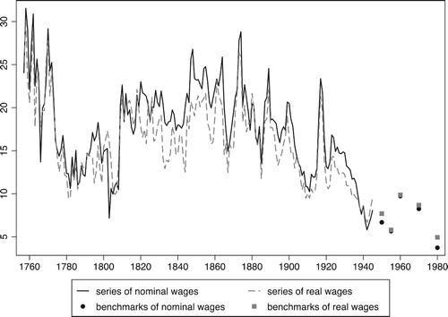
Whether we place the focus on nominal or real wages, the overall decline in the spread of wages across counties is quite remarkable. As Figure 1 shows, the coefficient of variation of nominal wages declined from about 19 in 1813 to 4 in 1980 (24 counties). The fall in the coefficient of variation was even larger if we examine the change starting in 1757, when the coefficient of variation stood at 28 (17 counties).¹¹ The real-wage measure of wage dispersion is somewhat lower throughout and confirms the downward trajectory from the beginning to the end; to remove cost-of-living differentials from nominal wage differentials does not affect our judgement of the long-term record of convergence.

By visual inspections, we may distinguish three distinct periods of wage convergence: from the late 1750s to the end of the Napoleonic wars, from the 1860s to the First World War, and during the 1930s and 1940s. The first and last convergence waves were followed by periods of quite stable wage dispersion, while the convergence wave in the late nineteenth and early twentieth century was followed by the turmoil during the First World War and the economic depression in the early 1920s.¹²

In Tables 1–5 that present the result of our statistical analysis of convergence, we have, beside the long run, several sub-periods that are justified largely by exogenous factors, such as considerations of the quality of the data, institutional changes affecting the spread of county wages, and the received wisdom about Swedish economic history. A more thorough discussion of these institutional factors appears in section 6 of this paper, and in Appendix 1 we offer further details of data considerations. In short, the first break point of 1776 was chosen because of the three institutional changes in the mid-1770s that might have affected the movement of county wages: (i) the minting reform; (ii) an amendment in the price setting of market price scales, whereby, besides the price level in towns, prices in rural areas would also influence the market price scales; and (iii) the repeal of the import restrictions on the domestic grain trade. The choice of the second break point of 1813 is justified upon data considerations. It is the first year that has the entire sample of county wages. The next one, that of 1865, is also related to data considerations. This is the year in which we change from Jörbergs market price scales to the official wage statistics, implying a discontinuity in the wage levels. We share the third break point of 1913 with several other studies of convergence (Table 6); in addition, this year implies the beginning of the macro-economic disturbances of World War I (Figure 1). The fourth break point of 1932 is motivated by important political and institutional changes in Sweden that affected the conditions for farm workers (Lundh & Prado, 2015). The fifth break point of 1955 is justified by the introduction of the solidaristic wage policy.

Table 1. Sigma-convergence.

Period	Nominal wages		Real wages
	Time coeff.	R^2	Time coeff.	R^2
	SE	P > |t|	SE	P > |t|
The long run
1757–1980 (a)	−0.0027	0.19	−0.0028	0.25
	0.0004	0.000	0.000	0.000
1813–1980 (c)	−0.0065	0.55	−0.0057	0.53
	0.0005	0.000	0.000	0.000
1865–1980 (c)	−0.0116	0.64	−0.0101	0.64
	0.0009	0.000	0.001	0.000
Sub-periods
1757–1776 (d)	−0.0250	0.36	−0.0235	0.37
	0.0079	0.005	0.007	0.004
1776–1813 (b)	0.0043	0.23	0.0095	0.25
	0.0035	0.232	0.003	0.001
1813–1864 (c)	0.0040	0.27	0.0013	0.02
	0.0009	0.000	0.001	0.354
1865–1913 (c)	−0.0105	0.41	−0.0108	0.39
	0.0018	0.000	0.002	0.000
1913–1932 (c)	−0.0041	0.02	−0.0077	0.05
	0.0072	0.578	0.008	0.344
1932–1955 (c)	−0.0385	0.73	−0.0226	0.64
	0.0063	0.000	0.005	0.000
1955–1980 (c)	−0.0214	0.31	−0.0112	0.14
	0.0227	0.444	0.020	0.625

Note: Following formula 1.

(a) 17–24 counties; (b) 20–24 counties; (c) 24 counties; (d) 17–20 counties.

Table 2. Beta-convergence: nominal wages.

Period	Model	Conv. rate	S.E.	P > |t|	R^2	Prob > F
The long run
1757–1980 (a)	UC	0.019	0.00014	0.000	0.99	0.000
	C1	0.019	0.00012	0.000	0.99	0.000
	C2	0.020	0.00014	0.000	0.99	0.000
	C4	0.019	0.00012	0.000	0.99	0.000
1813–1980 (c)	UC	0.032	0.00026	0.000	0.96	0.000
	C1	0.019	0.00027	0.000	0.97	0.000
	C2	0.034	0.00027	0.000	0.96	0.000
	C4	0.019	0.00028	0.000	0.97	0.000
1865–1980 (c)	UC	0.026	0.00035	0.000	0.96	0.000
	C1	0.032	0.00056	0.000	0.97	0.000
	C3	0.027	0.00036	0.000	0.97	0.000
	C5	0.030	0.00075	0.000	0.97	0.000
Moran’s I (1865–1980)	UC	Chi 2=	0.32	Prob. HO	0.5729
	C1	Chi 2=	0.28	Prob. HO	0.5988
	C3	Chi 2=	0.42	Prob. HO	0.5193
	C5	Chi 2=	0.28	Prob. HO	0.5988
Sub-period
1757–1776 (a)	UC	0.088	0.00475	0.000	0.84	0.000
	C1	0.105	0.00611	0.000	0.82	0.000
	C2	0.107	0.00656	0.000	0.78	0.000
	C4	0.105	0.00646	0.000	0.82	0.002
1776–1813 (b)	UC	0.098	0.00713	0.002	0.43	0.002
	C1	0.024	0.00692	0.034	0.64	0.001
	C2	0.120	0.00717	0.002	0.46	0.006
	C4	0.024	0.00672	0.031	0.68	0.001
1813–1864 (c)	UC	0.019	0.00513	0.027	0.20	0.027
	C1	0.018	0.00326	0.002	0.75	0.000
	C2	0.019	0.00524	0.031	0.21	0.083
	C4	0.020	0.00338	0.002	0.76	0.000
1865–1913 (c)	UC	0.021	0.00197	0.000	0.67	0.000
	C1	0.034	0.00201	0.000	0.87	0.000
	C3	0.027	0.00281	0.000	0.80	0.000
	C5	0.039	0.00263	0.000	0.88	0.000
1913–1932 (c)	UC	0.000	0.00536	0.998	0.00	0.998
	C1	0.028	0.00879	0.023	0.32	0.051
	C3	0.000	0.00644	0.996	0.20	0.353
	C5	0.023	0.00948	0.066	0.41	0.122
1932–1955 (c)	UC	0.069	0.00388	0.000	0.78	0.000
	C1	0.071	0.00870	0.001	0.80	0.000
	C3	0.057	0.00423	0.000	0.83	0.000
	C5	0.069	0.00845	0.001	0.84	0.000
1955–1980 (c)	UC	0.095	0.00554	0.000	0.66	0.000
	C1	0.135	0.00604	0.000	0.71	0.000
	C3	0.103	0.00616	0.000	0.67	0.000
	C5	0.115	0.00691	0.000	0.71	0.001

Note: Following formulas 2 and 3. (a) 17 counties; (b) 20 counties; (c) 24 counties. UC = Unconditional model; C1 = Conditional model 1: NUTS; Conditional model 2: the relative size of the urban population; C3 = Conditional model 3: the relative size of the urban population + the relative size of the industrial labour force + total migration rate; Conditional model 4: C1 + C2; Conditional model 5: C1 + C3.

Table 3. Beta-convergence: real wages.

Period	Model	Conv. rate	S.E.	P > |t|	R^2	Prob > F
The long run
1757–1980 (a)	UC	0.0143	0.00015	0.000	0.98	0.000
	C1	0.0141	0.00015	0.000	0.98	0.000
	C2	0.0137	0.00015	0.000	0.98	0.000
	C4	0.0131	0.00015	0.004	0.99	0.000
1813–1980 (c)	UC	0.0382	0.00033	0.000	0.94	0.000
	C1	0.0283	0.00035	0.000	0.95	0.000
	C2	0.0339	0.00034	0.000	0.94	0.000
	C4	0.0219	0.00036	0.000	0.95	0.000
1865–1980 (c)	UC	0.0412	0.00063	0.000	0.90	0.000
	C1	0.0274	0.00077	0.000	0.91	0.000
	C3	0.0270	0.00057	0.000	0.95	0.000
	C5	0.0216	0.00095	0.000	0.92	0.000
Moran’s I (1865–1980)	UC	Chi 2=	0.00	Prob. HO	0.9493
	C1	Chi 2=	0.30	Prob. HO	0.5854
	C3	Chi 2=	0.81	Prob. HO	0.3677
	C5	Chi 2=	0.28	Prob. HO	0.3804
Sub-period
1757–1776 (a)	UC	0.1098	0.00504	0.000	0.85	0.000
	C1	0.1083	0.00582	0.000	0.84	0.000
	C2	0.1086	0.00576	0.000	0.82	0.000
	C4	0.1120	0.00616	0.000	0.84	0.000
1776–1813 (b)	UC	0.0150	0.00748	0.141	0.12	0.141
	C1	0.0190	0.00678	0.061	0.44	0.023
	C2	0.0206	0.00758	0.074	0.21	0.138
	C4	0.0256	0.00621	0.018	0.58	0.008
1813–1864 (c)	UC	0.0213	0.00371	0.002	0.26	0.002
	C1	0.0147	0.00298	0.000	0.68	0.000
	C2	0.0207	0.00384	0.003	0.36	0.009
	C4	0.0148	0.00319	0.004	0.68	0.000
1865–1913 (c)	UC	0.0285	0.00267	0.000	0.61	0.000
	C1	0.0327	0.00221	0.000	0.84	0.000
	C3	0.0386	0.00301	0.000	0.80	0.000
	C5	0.0342	0.00267	0.000	0.87	0.000
1913–1932 (c)	UC	0.0042	0.00648	0.542	0.02	0.542
	C1	0.0310	0.00877	0.015	0.35	0.033
	C3	0.0064	0.00834	0.479	0.24	0.238
	C5	0.0297	0.00967	0.031	0.47	0.060
1932–1955 (c)	UC	0.0875	0.00511	0.000	0.71	0.000
	C1	0.0417	0.00951	0.011	0.74	0.000
	C3	0.0749	0.00611	0.000	0.78	0.000
	C5	0.0446	0.00989	0.012	0.79	0.000
1955–1980 (c)	UC	0.0479	0.00669	0.000	0.44	0.000
	C1	0.0466	0.00645	0.000	0.53	0.002
	C3	0.0548	0.00755	0.001	0.46	0.014
	C5	0.0496	0.00715	0.001	0.57	0.014

Note: See Table 2.

Table 4. Beta convergence from panel regressions: annual nominal wages.

	(1)	(2)	(3)	(4)	(5)	(6)
	1757–1945	1757–1776	1776–1813	1813–1864	1865–1913	1913–1932
Fixed effects
Lagged ln nominal wage	0.820***	0.593***	0.653***	0.770***	0.611***	0.583***
	(0.0226)	(0.0531)	(0.0367)	(0.0279)	(0.0352)	(0.0373)
Constant	0.392***	0.830***	0.904***	1.054***	1.794***	2.304***
	(0.0718)	(0.136)	(0.0942)	(0.118)	(0.167)	(0.203)
Convergence rate (%)	20	52	43	26	49	54
County FE	YES	YES	YES	YES	YES	YES
Year FE	YES	YES	YES	YES	YES	YES
R-squared	0.995	0.727	0.961	0.898	0.926	0.988
System GMM
Lagged ln nominal wage	0.809***	0.787***	0.771***	0.775***	0.906***	0.970***
	(0.0456)	(0.0932)	(0.0493)	(0.0383)	(0.0171)	(0.00749)
Constant	0.378***	0.422**	0.637***	1.030***	0.470***	0.178***
	(0.0915)	(0.183)	(0.126)	(0.158)	(0.0903)	(0.0406)
Convergence rate (%)	21	24	26	25	10	3
Wages instrumented	Lag 2	Lag 2	Lag 2	Lag 2	Lag 2	Lag 2
Year FE	YES	YES	YES	YES	YES	YES
Observations	4,282	334	799	1,247	1,176	480
Number of county	24	19	23	24	24	24

Note: Robust standard errors. Second lags of the levels and differences used as instruments. One-step estimates are reported.

***p < 0.01, **p < 0.05, * p < 0.1.

Table 5. Beta convergence from panel regressions: annual real wages.

	(1)	(2)	(3)	(4)	(5)	(6)
	1757–1945	1757–1776	1776–1813	1813–1864	1865–1913	1913–1932
Fixed effects
Lagged ln nominal wage	0.786***	0.529***	0.561***	0.715***	0.579***	0.597***
	(0.0273)	(0.0636)	(0.0298)	(0.0359)	(0.0362)	(0.0421)
Constant	0.987***	2.230***	2.284***	1.549***	2.270***	2.424***
	(0.155)	(0.347)	(0.152)	(0.175)	(0.197)	(0.245)
Convergence rate (%)	24	64	58	34	55	52
County FE	YES	YES	YES	YES	YES	YES
Year FE	YES	YES	YES	YES	YES	YES
R-squared	0.955	0.599	0.722	0.752	0.895	0.786
System GMM
Lagged ln nominal wage	0.731***	0.768***	0.607***	0.707***	0.821***	0.963***
	(0.0530)	(0.0812)	(0.0587)	(0.0577)	(0.0247)	(0.00917)
Constant	1.183***	1.039**	2.008***	1.483***	1.016***	0.174***
	(0.267)	(0.417)	(0.297)	(0.287)	(0.131)	(0.0565)
Convergence rate (%)	31	26	50	35	20	4
Wages instrumented	Lag 2	Lag 2	Lag 2	Lag 2	Lag 2	Lag 2
Year FE	YES	YES	YES	YES	YES	YES
Number of county	24	19	23	24	24	24
Observations	4,282	334	799	1,247	1,176	480

Note: Robust standard errors. Second lags of the levels and differences used as instruments. One-step estimates are reported.

***p < 0.01, **p < 0.05, *p < 0.1.

Table 6. Periods of convergence and divergence of regional wages in agriculture.

Study	Country	Convergence	Stable/divergence
Hunt (1973)	Britain	1867/70–1898
Jörberg and Bengtsson (1981)	Sweden		1835/44–1890/99
Söderberg (1985)	Sweden		1840–1910
	Britain	1840–1910
Boyer and Hatton (1997)	Britain		1855–1903
Heikkinen (1997)	Finland	1886–1913
Enflo et al. (2014)	Sweden	1860–1913	1913–1930
		1930–1940
This study	Sweden	1757–1813	1813–1864
		1865–1913	1913–1932
		1932–1980

We begin with the statistical test of σ-convergence, which takes the shape of a log-linear regression formula, as (1)(1) $\ln \left(\mathrm{C}{\mathrm{V}}_t\right)=\alpha +\text{β}\left(\mathrm{T}\mathrm{I}\mathrm{M}{\mathrm{E}}_t\right)+{\epsilon }_t$(1)

in which $CV$ is the coefficient of variation at $t$, $\mathrm{T}\mathrm{I}\mathrm{M}\mathrm{E}$ is the order of time at $t$ _, and $\epsilon$ is the error term at $t$. Sigma convergence occurs if the cross-sectional dispersion in wages declines over time. A negative and statistically significant coefficient for time indicates σ-convergence (Federico, 2012).¹³

Table 1 displays the test for σ-convergence in the long run and for sub-periods. The long-run tendency is clearly one of diminishing wage differentials, since the coefficient for time is negative and statistically significant, both for nominal and real wages. Typically, wage dispersion is larger in nominal than in real terms, indicating that regional variation in cost of living accounts for some of the dispersion in nominal wages. For the entire period (1757–1980), the coefficient of variation in nominal wages declined at an average rate of 0.3 percent annually. The rate of decline was faster, about 1.2 percent on average, during the industrial period (1865–1980).

Although the general trend was one of wage convergence, some periods showed another pattern. In 1776–1813, regional wage dispersion tended to increase from 13–14 percent to about 20 percent. In 1813–1864, it was quite stable until the end of the 1840s, when wage spread started to increase again. Another deviant period was in 1913–1932, during which differences in agrarian county wages first increased around the beginning of the First World War, second declined, and then increased anew during the economic depression in 1920–1922. Thereafter, differences stabilised in the early 1930s at the pre-war level, before declining in the 1930s and 1940s. Moreover, the rate of convergence ranged widely between periods and was faster in 1757–1776 (2.5 percent per year for nominal wages), in 1865–1913 (1.1 percent per year), in 1932–1955 (3.9 percent per year), and in 1955–1980 (2.1 percent per year).¹⁴ The period 1932–1955 stands out with the highest rate of convergence.

4. Beta convergence by cross-sectional design

Besides σ-convergence, we also enquired into the magnitude of β-convergence, a regression coefficient that establishes the speed at which low-wage regions outgrow high-wage regions. In the parlance of the convergence literature, we seek a negative correlation between high level of initial income and growth potential – the benefits of backwardness, so to speak (Abramovitz, 1986). The great advantage of the method is that it only requires data for benchmark years. It has therefore been widely used in studies of regional wage convergence, which in turn facilitates international comparisons.

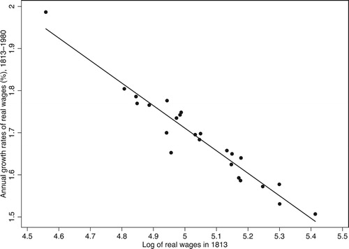
Figures 2 and 3 illustrate the strength of β-convergence. They show scatter plots of the negative relationship between growth rates of county-specific wages in 1813–1980, as well as the log of the wage levels in 1813, the first year hosting all the 24 counties. Figure 2 plots wages in nominal terms and Figure 3 plots wages in real terms. With few exceptions, relatively low wage levels in 1813 were associated with faster than average growth rates in the period as a whole. The benefits of backwardness translated into higher than average growth rates for low-wage regions and lower than average for high-wage regions.

Figure 2. Annual growth rates of nominal county wages in 1813–1980 vs. the log of nominal county wages in 1813.

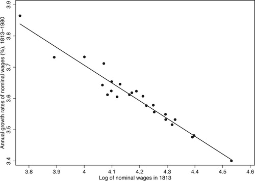
Figure 3. Annual growth rates of real county wages in 1813–1980 vs. the log of real county wages in 1813.

The statistical test of β-convergence, which has been frequently used in research on regional wage convergence since Baumol (1986), proceeds in two steps. The first is defined as (2):(2) $\frac{1}{T}\ln \left(\frac{\mathrm{W}\mathrm{a}\mathrm{g}{\mathrm{e}}_{c,\mathrm{f}\mathrm{i}\mathrm{n}\mathrm{a}\mathrm{l}}}{\mathrm{W}\mathrm{a}\mathrm{g}{\mathrm{e}}_{c,\mathrm{i}\mathrm{n}\mathrm{i}\mathrm{t}\mathrm{i}\mathrm{a}\mathrm{l}}}\right)=\alpha +\theta \ln \left(\mathrm{W}\mathrm{a}\mathrm{g}{\mathrm{e}}_{c,\mathrm{i}\mathrm{n}\mathrm{i}\mathrm{t}\mathrm{i}\mathrm{a}\mathrm{l}}\right)+{\epsilon }_c$(2) in which T is the number of years in each period, and $\mathrm{W}\mathrm{a}\mathrm{g}{\mathrm{e}}_{c,\mathrm{i}\mathrm{n}\mathrm{i}\mathrm{t}\mathrm{i}\mathrm{a}\mathrm{l}}$and $\mathrm{W}\mathrm{a}\mathrm{g}{\mathrm{e}}_{c,\mathrm{f}\mathrm{i}\mathrm{n}\mathrm{a}\mathrm{l}}$ are the wages of day workers in county c in the initial and final years of the period, respectively. The estimated regression coefficient ($\theta$) expresses the relationship between growth rates and the level of the first year in a natural logarithm. The Unconditional Convergence model predicts convergence without controlling for any county-specific characteristics. It thus assesses the joint effects of within- and between-county convergence (Barro & Sala-i-Martin, 1991; Rosés & Sánchez-Alonso, 2004).

Formula (2) may be transformed from an unconditional to a conditional convergence model by the inclusion of additional control variables, $\gamma X_c$, as in the specifications of models C1–C5 in Tables 2 and 3. The test for conditional β-convergence follows the formula (3):(3) $\frac{1}{T}\ln \left(\frac{\mathrm{W}\mathrm{a}\mathrm{g}{\mathrm{e}}_{c,\mathrm{f}\mathrm{i}\mathrm{n}\mathrm{a}\mathrm{l}}}{\mathrm{W}\mathrm{a}\mathrm{g}{\mathrm{e}}_{c,\mathrm{i}\mathrm{n}\mathrm{i}\mathrm{t}\mathrm{i}\mathrm{a}\mathrm{l}}}\right)=\alpha +\theta \ln \left(\mathrm{W}\mathrm{a}\mathrm{g}{\mathrm{e}}_{c,\mathrm{i}\mathrm{n}\mathrm{i}\mathrm{t}\mathrm{i}\mathrm{a}\mathrm{l}}\right)+\gamma X_c+{\epsilon }_c$(3) The conditional model makes it possible to determine how the introduction of controls affects the estimated rate of convergence. If including a control variable entails a reduction in the size of $\theta$ relative to the unconditional model, we conclude that the control variables add to convergence. In this case, the unconditional model has over estimated the rate of convergence. If, in contrast, including control variables entails an expansion in the size of $\theta$ relative to the unconditional model, the control variables add to divergence. In that case, the unconditional model has under estimated the rate of convergence.

In the second step, the annual speed of convergence, $\text{β}$, is defined as (4):(4) $\mathrm{A}\mathrm{n}\mathrm{n}\mathrm{u}\mathrm{a}\mathrm{l}\mathrm{s}\mathrm{p}\mathrm{e}\mathrm{e}\mathrm{d}\mathrm{o}\mathrm{f}\mathrm{c}\mathrm{o}\mathrm{n}\mathrm{v}\mathrm{e}\mathrm{r}\mathrm{g}\mathrm{e}\mathrm{n}\mathrm{c}\mathrm{e}\left(\text{β}\right)=-\left(\frac{1}{T}\right)\ln (\theta T+1)$(4) in which $\theta$ is the regression coefficient from (2) or (3) and, thus defined, the coefficient is a positive value expressing the annual speed of convergence (Barro & Sala-i-Martin, 1991).¹⁵

Our model of conditional β-convergence includes three specifications. Conditional model 1 controls for county differences in geographic location. We classified counties as East, North or South according to level 1 of the classification scheme employed by Nomenclature des Unités Territoriales Statistiques (NUTS). The North sample includes counties in Northern and Central Sweden, where the mining, wood, and paper and pulp industries are common. The East and South samples include counties that have a more diversified industrial structure, barring the predominance of metal industries in the East. They also differ from the North with regard to the presence of large cities, such as Stockholm (East), and Gothenburg and Malmö (South).

Conditional model 2 controls for the degree of urbanisation. Urbanisation is measured as the share of people residing in urban areas in the period 1757–1960. In the period 1960–1980, it is represented by the percentage of those living in densely populated areas (tätorter).¹⁶

Conditional model 3 controls for county differences in the degree of urbanisation, the degree of industrialisation, and the level of net total migration. Industrialisation in the period 1865–1913 is measured as the proportion of the population who earned their living from industry; in the period 1920–1980, it is represented by the percentage of industrial workers among those who were employed.¹⁷ Migration is represented by the net total immigration per 1,000 in the mean county population, which is the difference between the internal and external in-migration minus the difference between the internal and external out-migration divided by the county population times 1,000.¹⁸

Conditional model 4 includes the control variables of models 1 and 2: geographic location and the relative size of the urban population. Conditional model 5 includes all variables of models 1 and 3: geographic location, the relative size of the urban population, the relative size of the industrial labour force, and the net total migration rate.

Tables 2 and 3 set out the regression results for nominal wages and real wages. They also include the i-Moran test that controls for spatial dependence. We have performed the test for the longest sub-period covering all 24 counties using an inverse-distance weighing matrix. The test fails to detect any spatial dependence of the residuals. Spatial correlation by wages may be low because the counties are fairly large.

Overall, the long-run path conforms to β-convergence whether examining nominal or real wages. Beginning with nominal wages, for the industrial period (1865–1980), the rate of convergence was 2.6–3.2 percent per year depending on the model, which indicates that the average annual convergence rate was about 3 percent. For the very long-term period 1757–1980, the annual convergence rate was somewhat lower, about 2 percent per year.¹⁹ For the period 1813–1980, including all 24 counties, the point estimate of β varied between 2 and 3 percent per year.

Turning to the regression results for real wages, displayed in Table 3, we find a similar pattern. The convergence rate was 2.2–4.1 percent per year (depending on model) in the industrial period 1865–1980, and lower for periods starting earlier. Since the estimated convergence rates were lower for all conditional models compared to the unconditional model, we conclude that geographic location, urbanisation, industrialisation, and migration were related to long-run real wage convergence of real county wages of farm workers. The unconditional model hence overestimates the rate of convergence.

These long-term rates of annual convergence can be interpreted in light of the findings of previous research on regional GDP per capita. Studies have concluded that β-estimates cluster around two percent (Barro & Sala-i-Martin, 1995). Our long-term estimates are somewhat lower, but since they begin in the eighteenth or early nineteenth century it is reasonable to assume that they would show different magnitudes. With an annual convergence rate of two percent, it takes about 35 years to eliminate half of the dispersion, according to the half-life formula: −ln0.5/β. Meanwhile, the long-term estimates conceal a great deal of inter-temporal variations that provide important information on the progression of labour market integration.

We now turn to the lower panel of Table 2, which reports the estimates of the convergence rates of nominal wages for shorter sub-periods. It is clear that the β-coefficient was positive and statistically significant, indicating β-convergence for all sub-periods but the one between 1913 and 1932. Yet the annual rate of convergence varied across sub-periods: it ranged between 2.1 and 3.9 percent in 1865–1913, 5.7 and 7.1 percent in 1932–1955, and 9.5 and 13.5 in 1955–1980 (depending on the model used). We can also see a substantial rate of β-convergence for the period 1813–1865, characterised either by low levels of σ-convergence or no convergence at all. The patterns formed by the estimated rates of convergence across periods are similar for real wages and nominal wages. The annual rate for real wages varied between 2.9 and 3.9 percent in 1865–1913, 4.2 and 8.8 percent in 1932–1955, and 4.7 and 5.5 percent in 1955–1980.

Our results so far show that the tests for σ-convergence and β-convergence reported in Tables 1–3 match the graphical representation of long-term wage convergence in Figures 1–3. Catching-up growth among low-wage counties was a major driver of convergence in the entire period, barring the years between 1913 and 1932, when β-convergence did not manifest itself.

5. Beta convergence by panel-data design

Even though the cross-sectional design of β-convergence has useful attributes in historical research – for instance, it does not require annual data – recent developments in econometrics have shown that its simplicity may come at a price. Islam (1995) criticises the cross-sectional specification because it gives rise to a systematic downward bias in the estimated magnitude of β-convergence. The cross-sectional specification fails to control for unobserved regional characteristics that influence the long-run steady state of each region. The potential influence of unobserved characteristics explains why panel data models have gained ground in convergence studies. Panel models enable researchers to control for time-invariant heterogeneity by using fixed effects.

The interpretation of the convergence coefficient with panel data is different. With the cross-sectional design, the estimated coefficient indicates all counties’ average speed of convergence towards the sample mean; in contrast, with the panel data design, the estimated coefficient indicates the average speed of convergence towards the long-run equilibrium, taking other unobserved regional differences into account. Typically, the estimated β-coefficient in panel data models is larger, indicating faster convergence than the standard rate of 2 percent a year suggested by Barro and Sala-i-Martins (1991, 1995). de la Fuente (2002), for instance, estimates that the speed of convergence was about 12 per cent per annum in Spanish regions for the post-war period. Canova and Marcet (1995) report that the convergence rate was 23 percent per annum when each Spanish region was allowed to converge to its own steady state growth rate in the post-World War II era.

Since we have annual data for most of the period under consideration in this study (1757–1945), we have designed a complementary test of convergence using panel data. Thus, in order to buttress the view that Swedish regional wage convergence was substantial since 1757, established by the cross-sectional specification, we have examined the rate of convergence by means of a panel-data model of conditional β-convergence, using the same time spans of the previous section. We have created a panel-data model of conditional β-convergence in regional wages as in Formula (5),(5) $\mathrm{\Delta }{w}_{i,t}=\left(\text{β}-1\right)w_{i,t-1}+{\eta }_i+{\lambda }_t+{\epsilon }_{i,t}$(5) where $\mathrm{\Delta }$ is the difference operator between $t$ and $t-1$, $w$ is the log of real or nominal wage in county $i$ at time $t$, $\eta$ are regional fixed effects, and $\lambda$ are time-specific dummies. The time-specific dummies are included to control for period-specific trends in wage growth that might otherwise generate spurious results. The convergence parameter of interest is $\left(\text{β}-1\right)$, which measures the relationship between the changes in wages from $t$ to $t-1$ on the left hand side of the equation, and the lagged wage rate on the right hand side.

The estimated coefficient, $\text{β}$, indicates the speed of convergence, and is calculated as(6) $\mathrm{A}\mathrm{n}\mathrm{n}\mathrm{u}\mathrm{a}\mathrm{l}\mathrm{s}\mathrm{p}\mathrm{e}\mathrm{e}\mathrm{d}\mathrm{o}\mathrm{f}\mathrm{c}\mathrm{o}\mathrm{n}\mathrm{v}\mathrm{e}\mathrm{r}\mathrm{g}\mathrm{e}\mathrm{n}\mathrm{c}\mathrm{e}\left(\text{β}\right)=-\ln \left(\text{β}\right)$(6) Panel data models with fixed effects might give rise to biased estimates of convergence rates. The reason is that the lagged dependent variable on the right-hand side of Formula (5) could be endogenous in the presence of first order auto-correlation in the residuals. To remedy this problem, we follow Enflo et al. (2014), and provide estimates that are based on system GMM with lags in levels and differences in order to instrument for the potentially endogenous wage variable.

Tables 4 and 5 display the results of panel regressions based on annual county wages of male farm workers. The upper part of the panel shows the results based on panel data with fixed effects; and the lower part of the panel shows the same regressions using system GMM. The tables show that the fixed-effect model yields convergence rates that are somewhat over-estimated. The model that applies system GMM modifies the estimated rates somewhat, but these rates are still much larger compared to the rates of the cross-sectional estimates (Tables 3 and 4).

The first column (1) of the two tables records the longest possible time span with annual data (1757–1945), while the following ones (2–6) record the same sub-periods as for the cross-sectional design. In general, we found that the implied yearly rate of convergence, defined as in Formula (6), was faster than in the cross-sectional specification (unconditional and conditional model). The difference between nominal and real terms is negligible. For the longest period possible with annual data (1757–1945), we estimated an annual convergence rate of 20 percent for nominal wages and of 24 percent for real wages (fixed effects). There are some noteworthy differences, however, in particular for the 1913–1932 period. The cross-sectional design estimated no convergence for this period; the panel data design with fixed effect estimated very rapid convergence rates; and the system GMM design estimated rates that are somewhere in between. To understand this incongruence among the three measures, we must recall that the panel-data approach permits the estimation of different convergence rates to different steady-state growth rates for each county. Convergence of each county to its own steady-state wage level may be very fast despite invariant cross-sectional differences. In addition, the fixed effects estimator could have an upward bias in the presence of autocorrelation. Once we have corrected for autocorrelation, the system GMM design suggests a modest convergence rate at 3 per cent annually.

The panel-data design does not reveal anything about cross-sectional differences. Between 1913 and 1932, cross-sectional differences persisted because macro-economic disturbances were unfavourable to convergence. Yet each county quickly reverted to its own steady-state growth path. Thus, it is reasonable to assume that regional differentials in human and social capital, geography or factor endowments explain much of the variety in regional-specific growth rates.

6. Discussion of convergence regimes

Our empirical analysis so far, based on several measures of convergence, has identified three waves of regional wage convergence among agrarian workers, 1757–1813, 1865–1913, and 1932–1980, along with spells of stability or divergence between these periods. Since our study is unique in regard to the first and third convergence waves, only the second wave of convergence can be compared with previous studies. The converging wages that stretched from the industrial breakthrough to the First World War, shown in Table 6, correspond with the results of previous studies on Finland (Heikkinen, 1997), Sweden (Enflo et al., 2014), and Britain (Hunt, 1973; Söderberg, 1985). Furthermore, the pattern of wage dispersion among agrarian workers found in our study corresponds well with what we found in a previous study of manufacturing workers in Sweden: convergence in 1860–1912 and 1931–1983, and divergence in 1912–1931 (Collin et al., 2019). For the rest of this section, we delve into the historical context of the regional wage spread of farm workers, especially in relation to markets and institutions.

6.1. Convergence: mid eighteenth to early nineteenth century

Convergence and volatility mark the evolution of regional wages from mid eighteenth century to early nineteenth century.²⁰ Migration can be ruled out as a possible factor behind this convergence for two reasons: the transport revolution had not taken place yet; most internal migration was circular and local, and not long distance or across county borders. A possible factor propelling regional wage convergence is market integration of grain, which affected wages indirectly. According to the theorem of factor price equalisation, convergence of commodity prices will also lead to convergence in wages. It is thus worthwhile to list the forces that might have propelled commodity price integration. The first one, as various authors have pointed out, is the 1775 repeal of import restrictions on domestic grain trade (Ahlström, 1974; Utterström, 1957). Second, imports of grain from foreign countries might also have played an important role, since the various ports along the Swedish coast facilitated grain imports. It is therefore likely that the Swedish price integration has adjusted to international prices (Berg, 2007; Olsson, 2002; Rantanen, 1997, p. 217). Third, if the tax burden of peasants increased, they would have had to buy more grain in order to pay taxes, which in turn would have increased the flow of grain from surplus to deficit areas. The tax burden generally decreased between 1735 and 1765 (Herlitz, 1974, p. 255), and there is some evidence that it might have increased thereafter (Olsson, 2005). In sum, the regional integration of grain markets made the regional spread in costs of living and product prices decrease; as a result, the regional real wage dispersion in agriculture diminished.

6.2. Stability: from first to third quarter of the nineteenth century

The period following the drastic decline in wage differentials, coinciding largely with the first three quarters of the nineteenth century, is not subject to wide swings in either direction. Instead, low volatility and stability in the size of the coefficient of variation are distinguishing features of the development of regional labour market integration during this period. Between 1813 and 1872, the coefficient of variation fluctuated at an average of 20 percent. During the nineteenth century, changes in labour market institutions paved the way for a modern labour market in agriculture. Individual employment contracts between two equal parties replaced older forms of coercive labour relations on the manors, and cash wages and short-term notice replaced payments in kind and yearly employment periods (Lundh, 2010). Sweden was still overwhelmingly rural, and the impact of manufacturing on the wages of farm workers was negligible at least until the 1850s, when the sawmills along the Northern Baltic coast began to grow. The rapid growth of the manufacturing sector in the fourth quarter of the nineteenth century marks the end of the period of stability and the beginning of the second period of convergence.

6.3. Convergence: from 1860s to World War I

The second wave of regional wage convergence stretched from the 1860s to the First World War. Regional wage convergence in agriculture was driven mainly by internal migration and emigration up to the First World War (Enflo et al., 2014). Besides, internal migration affected the demand for and supply of labour in the industrial and agricultural labour markets, leading to a decline in the industrial-agrarian wage gap. By the 1910s, industrial wages were somewhat higher because of the higher unemployment risk in industry (Lundh & Prado, 2015). A long-term perspective on the wage gap shows that a state of equilibrium had been achieved before the outbreak of World War I. Another sign of the growing interconnection between the industrial and agrarian labour markets was the greater volatility in agrarian wages. This volatility stemmed from industrial business cycles, manifested most notably in the buoyant market for the saw mill industry during the mid 1870s. Saw mills competed with agriculture for day workers, which raised day workers’ wages (Bagge, Lundberg, & Svennilson, 1935, pp. 357–60; Cornell, 1982, pp. 168–9). Collin (2016, paper 3) has assessed the degree of correlation between farm wages and manufacturing wages across the 24 counties in 1860–1945. The correlation in the level of real and nominal wages of farm workers and manufacturing workers was subject to ups and downs, but it reached relatively high magnitudes at the outbreak of World War I and remained so until the late 1930s, testifying to an emerging market integration with recurrent backlashes.

The most discernible force underlying the levelling of wages was the large Swedish emigration. Sweden ranked second in per capita emigration in the late nineteenth and early twentieth century (Bohlin & Eurenius, 2010). Emigration had an impact on the regional wage structure by shifting the supply of workers across counties. Outmigration occurred mostly from low wage counties, which made wages grow faster in these counties than one would expect in the absence of migration. Sweden also had large internal migration rates. These internal flows of labour seeking pecuniary advantages occurred both within and between urban and rural areas. In addition, because of the slow rate of Swedish urbanisation, the so-called agglomeration forces were not yet sufficiently powerful to offset the levelling force of migration. As a result, migration served to even out inter-county wage differentials (Enflo et al., 2014).

6.4. Divergence: from World War I to the great depression

The outbreak of the First World War and the disorder that followed in its wake brought forth a dramatic, if short-term, increase in inter-regional wage differentials, manifested by σ-divergence and β-divergence. The coefficients of variation rose rapidly, and then bounced back immediately. In rural areas, the corollary of an economic shock – in this case, war-induced scarcity of food that raised food prices in favour of grain producing counties – was, once again, regional wage divergence on a large scale. It is likely that World War I and the macroeconomic – mostly monetary – disturbances in its aftermath delayed by a decade the process of wage convergence that was well under way since at least the turn of the century. The mid-1920s ended bouts of significant divergence owing to demand and supply imbalances, marking the beginning of the third and lasting sub-period in which most of the volatility and remaining differences disappeared. Notwithstanding the lack of σ-convergence and β-convergence according to our cross-sectional design, our panel-data estimate of β-convergence for this period indicates that the distribution of unobserved county-specific characteristics allowed each county to resume its own steady-state growth path quickly.

6.5. Convergence: from the early 1930s to 1980

The third wave of regional wage convergence in agriculture occurred from the 1930s to the end of mid-1950s. Apart from a brief interlude of divergence in the 1960s, convergence continued, implying that the coefficient of variation stood at an all-time low of 4–5 percent by the 1980s. Migration was substantial during this period, but it played a different role in convergence because the Swedish net out-migration was replaced by net immigration in the post-World War II era. In the 1940s, 1950s and 1960s, the Swedish Labour Board (Arbetsmarknadsstyrelsen, AMS) directed immigrating foreign workers and refugees mainly to the industrial sector, and only in rare cases to agriculture. Most of the asylum seekers of the 1970s were urban, and they seldom took up jobs in agriculture. Internal migration increased, but its direction was predominantly from rural to urban areas, as well as from agriculture to industry. The unambiguous drift towards urbanisation and depopulation of the countryside put pressure on agrarian employers to pay competitive wages in relation to industrial wages. Thus, both regional wages in industry and in agriculture converged from the early 1930s to the 1980s.

An important feature of the Swedish labour market is the high level of union density and collective bargaining coverage. Trade unions and collective agreements were established in the industrial sector in the late nineteenth and early twentieth century. Unionisation of rural workers progressed slowly but steadily during the interwar period. The late 1920s witnessed the first steps towards the creation of a national labour union for rural workers. Even though unionisation in agriculture never comprised the majority of workers and never came close to the coverage of the industrial sector, the increase in the 1930s and 1940s strengthened the bargaining power of rural workers and levelled the growth of wages across counties. Because collective agreements covered a growing share of workers, the wages of rural workers were no longer entirely defined by fluctuations in product markets.

Institutional arrangements affected wage convergence during World War II. Fear of galloping inflation compelled the Swedish Trade Union Confederation (LO) and the Swedish Employers’ Confederation (SAF) to negotiate terms and conditions for workers and employers during World War II. The result of these negotiations gave an additional boost to farm workers’ wages. In order to curb mounting inflation during the war, both confederations agreed to allow nominal wages to increase by 0.4 percentage points if the cost of living increased by 1 percent (Treslow, 1996, p. 57). In other words, they subscribed to a real wage drop during the war. However, the low-paid status of farm workers made them the subject of special treatment; SAF and LO agreed to refrain from imposing a cap on farm workers’ wages during the war. In addition, agricultural workers also received a fixed supplement to their cash wages between 1941 and 1944 (Casparsson, 1943, p. 22; Lönestatistisk årsbok för Sverige 1945, p. 32). These negotiations, Prado and Waara (2018) argue, constituted a deliberate attempt to favour the growth of wages for low-wage workers, and they anticipated the so-called solidaristic wage policy that would be put into practice in the 1950s. These institutional arrangements probably contributed to the decrease in regional wage differences of farm workers. A similar tendency of regional convergence is also visible for manufacturing workers as a whole (Collin et al., 2019).

Institutional arrangements also compressed the wage structure during the post-World War II period. The centralised wage negotiations between LO and SAF aiming at wage compression, which began during the Second World War, consolidated into a stable labour market institution between 1956 and 1982. This particular institutional arrangement, commonly described as a solidaristic wage policy, aimed at the compression of industrial wages by allowing a larger rise in payments to low-wage groups. The coordinated central wage bargaining had a significant geographical component. Low-wage groups were not randomly distributed among industrial branches, and industrial branches were not equally represented across counties. As a result, the policy increased the rate of convergence of regional wages in industry. Agriculture was not included in the system of coordinated collective wage bargaining, but it was indirectly influenced via the industrial sector. As regional wages in industry tended to converge, the convergence rate increased in agriculture.

The growing political clout of the agricultural sector since the 1930s affected regional wages of farm workers. The catalyst for change was the inferior social status of farm workers in the interwar period and the early post-World War II era, when manufacturing and urbanisation were adopted as political creeds, industrial workers were paid higher wages, urban life was celebrated, and social reforms benefitted mainly industrial workers. The demoralising effect of modernisation upon farm workers provides, somewhat unexpectedly, the backdrop to the formation of a counter-movement engaged in promoting the status of agriculture and the countryside. Rural organisations rallied to raise awareness about the problems that affected agriculture in general and the increasing income gap between their members and other worker groups in particular (Lundh & Prado, 2015). Farmers’ representatives succeeded very well in their quest for tight price controls and protection against foreign competition. Several regulations benefitting the agricultural sector were adopted between 1930 and 1935. Some of these benefits accrued to the peasant party for the support it gave to the Social Democrats in the agreement of 1933, popularly known as the Horse Trade deal (kohandeln) (Morell, 2001, p. 78 f.; Nyman, 1944). In 1936, the Swedish parliament passed a bill that reduced the weekly working time in agriculture to 52 hours. Farm workers had thereby received compensation for being sidestepped in 1919, when manufacturing workers benefitted from substantial reductions in working hours. The reduction applied to large farms but it also affected farms not covered by the collective bargaining system (Lundh & Prado, 2015, p. 74). The working hours reduction was responsible for a third of the hourly wage increase of 30–50 percent between 1934 and 1937 (Nyström, 1938; SOU, 1938:15, p. 158).

In summary, the post-war period witnessed the integration of labour markets for industrial and agrarian workers. Regional wages of manufacturing workers converged, partly because of the highly centralised collective bargaining system, and it is likely that this wage convergence in manufacturing, promoted by the solidaristic wage policy, affected regional wages of farm workers.

7. Conclusion: labour and the ‘law of one price’

We have compiled the longest series of nominal and real wages across regions so far, a necessary requisite for our assessment of regional labour market integration. The change in the magnitude of wage dispersion is quite remarkable. Regional wage differentials were a great deal larger in the third quarter of the eighteenth century than they were in 1980: the coefficient of variation declined from about 28 to 4 percent. In itself, this precipitous drop in the spread of wages across space marks one of the most profound changes in the function of the labour markets, with a lasting impact on income distribution and regional GDP per capita.

Research on price convergence often resorts to the metaphor of the ‘law of one price’ to describe how market forces, if unfettered, always eliminate price differentials of identical commodities across space. Given the almost complete elimination of regional wage differentials for farm workers revealed by our investigation, it is instructive to consider to what extent this metaphor is also applicable to labour markets. First, workers may simply disobey the rules of the market because they give preference to motives other than searching for pecuniary gains, which restrains labour mobility. Second, and most important for our investigation, wage convergence may just as well be the result of political and institutional arrangements: if the demand and supply forces of the market do not reign supreme, the metaphor loses its explanatory power.

Our study finds that the convergence in county wages was not caused by the mechanism attributable to ‘the law of one price’ alone. Rather, it was caused by markets and institutions interchangeably. Convergence occurred above all in three periods: in the late eighteenth century, the late nineteenth and early twentieth century, and in the 1940s. We have identified two sets of factors each of which propelled convergence in these three episodes. On the one hand, the early convergence episodes were driven largely by market factors, price integration of grain markets and emigration, which chimes in with the notion of convergence as a corollary to market forces. On the other hand, the final convergence episode was driven largely by politics and institutions, above all through unionisation in agriculture and centralised agreements in the industrial sector that indirectly affected agriculture. Hence, it was the combined force of both markets and institutions that drove wage convergence across the entire period, which calls into question the purported, straightforward link between labour market integration and the competitive forces associated with the ‘law of one price’.

Acknowledgements

A draft version of this paper was presented at the Swedish Economic History Meeting in Umeå, 2015. We appreciate the suggestions from the participants. A revised version was included as paper 2 in Kristoffer Collin's dissertation (Collin, 2016). The present version of the paper takes precedence over the previous versions. Moreover, we have received invaluable comments by Jakob Molinder, Sakari Heikkinen, Rodney Edvinsson, Stefan Öberg, Jan Bohlin, Martti Rantanen, Mats Olsson and three anonymous referees. We also thank Evelyn Prado for proof reading. We would like to acknowledge the financial support from Riksbankens Jubileumsfond and Jan Wallanders och Tom Hedelius Stiftelse/Tore Browaldhs Stiftelse, for the research projects ‘Swedish Wages in Comparative Perspective, 1860–2008’ (P09-0500:11-E) and ‘Swedish Wages 1860–2010 in labour economics perspective’ (P2011-0182:1). Kristoffer Collin and Svante Prado would also like to acknowledge individual financial support provided by Jan Wallanders och Tom Hedelius Stiftelse (W17-0032; W2009-0161:1).

Disclosure statement

No potential conflict of interest was reported by the author(s).

Additional information

Funding

This work was supported by Jan Wallanders och Tom Hedelius Stiftelse samt Tore Browaldhs Stiftelse: [Grant Number P2011-0182:1,W17-0032,W2009-0161:1]; Riksbankens Jubileumsfond: [Grant Number P09-0500:11-E].

Notes

1 At least since Todaro (1969) and Harris and Todaro (1970), the literature on rural to urban migration has recognized that rural workers base their migration decision on the expected incomes, hence future incomes conditioned on the risk of unemployment. Elimination of urban to rural wage differentials may therefore never occur. The literature on regional wage convergence strives instead to compare homogenous workers categories that might meet similar risks of unemployment.

2 For Sweden, see: Jörberg (1972a); Jörberg and Bengtsson (1981); Bengtsson (1990); Lundh, Schon, and Svensson (2005); Enflo et al. (2014). On wage convergence across regions, see for instance: Verma (1973); Rosenbloom (1990, 1998); Sicsic (1995); Boyer and Hatton (1997); Heikkinen (1997); Collins (1999); Margo (2004); Rosés and Sánchez-Alonso (2004). On convergence across countries and continents, see for instance: Allen (1994, 2001); Söderberg (1985); Williamson (1995); Curtis and Fitz Gerald (1996); Bértola and Williamson (2006); Prado (2010); Caruana Galizia (2015).

3 Supplementary materials can be found in Appendices 1 and 2, published online.

4 We use the label ‘official statistics’ to denote wage statistics published by Statistics Sweden (Statistiska Centralbyrån, SCB) or the Social Board (Socialstyrelsen) in the series Sweden's Official Statistics (SOS).

5 Between 1865 and 1936, daily wages for agricultural workers in the official statistics are classified by winter or summer wages. After 1936, the inter-temporal classification is more detailed. In addition, daily wages also specify whether the employment contract is permanent or temporary and whether rest and meal breaks counted as work hours. The wage series of day workers used here refer to day workers who brought their own food. Furthermore, the wage level is an average of winter and summer wages and an average of permanent and temporary day workers. A detailed account of the official wage statistics for farm workers appears in Lundh and Prado (2015, supplementary material).

6 For about half of the sample, the wage level is higher in Jörberg than in the official statistics. On average, however, wages are about 5 percent higher in Jörberg, driven by some counties where the wage level was much higher in Jörberg compared to the official statistics: Norrbotten, Västerbotten, Göteborg and Bohus, and Jämtland. A third source, Bagge et al. (1935), who also offer market price scales with important modifications, corroborates that Jörberg's wage levels are generally too high and imply too much variation. The ground for this assumption is Jörberg's inclusion of casual labour in urban areas for some of the 24 counties. Casual labour in towns probably earned a wage premium relative to casual labour in the countryside (see appendix 1 for further discussion).

7 In a similar study on manufacturing workers (Collin et al., 2019), the cost-of-living index was based on food prices and housing costs. We chose not to include the series on housing cost here because it is based mainly on city prices that would not be representative of the levels and the variation in rural housing costs.

8 Market price scales have been considered indicative of market transactions, at least after the 1760s, see Fridlizius (1957); Montelius, Utterström, and Söderlund (1959); Lindgren (1971); Ahlström (1974).

9 Population: Statistical Database of Sweden Statistics (BE0101N1).

10 Another measure of sigma convergence is the standard deviation of the log of wages. This has also been used by the previous literature on convergence, and has sometimes produced results that deviate from the coefficients of variation in quite dramatic ways, as Dalgaard and Vastrup (2001) have noted. We have, therefore, as a robustness check, computed the standard deviation of the log of nominal wages in order to see if the results would change significantly. For the whole period between 1757 and 1980, the difference is very small. If we set the two measures to 100 in 1857, the coefficient of variation arrives at 15.5 and the standard deviation of the log of wages at 12.7. There are some differences across the different sub periods but the pattern of convergence and divergence episodes would not be altered by changing measures.

11 In order to check the robustness of the calculations prior to the full-sample period (1813–1980), we estimated the coefficient of variation for the 17 counties included in 1957 and the 20 counties included in 1776, and compared it with the full-sample coefficient of variation that refers to the period 1813–1980 (not shown here). On average, the deviation from the full-sample coefficient of variation for the period 1813–1980 was about 4 percentage points for both samples, mostly because the high-level northern counties are included in the full sample. The long-term pattern of convergence and stability was similar. Hence, it seems reasonable to conclude that the gradual inclusion of counties completed in 1813 was not responsible for the overall downward tendency or for the reduced spread of wages after the 1750s.

12 As a check for the robustness of the national sigma convergence, we have computed sigma convergence for each of the three NUTS regions that we have used as controls in the beta convergence regressions (Tables 2 and 3). Largely, the movement of sigma convergence in the three regions followed the national pattern, but yearly fluctuations were larger since the number of counties included in each region was small (6, 7 and 11 respectively).

13 To check the robustness of the standard test of sigma convergence proposed by Federico (equation 1), we used another specification, Δ ln CV=α+β TIME+ψ ln CVt−1+ ϕ Δ ln CVt−1+εit, in which CV is the coefficient of variation at t, TIME is the order of time at t and ε is the error term at t. The change in the natural logarithm of CV at t is regressed on TIME at t, the natural logarithm of CV the previous year, and the change in the natural logarithm of CV the previous year. As for equation 1, a negative and statistically significant coefficient for time indicates σ-convergence. We ran the regressions using both models and found no difference in the characteristics of periods (not shown here).

14 All percentages refer to nominal wages; the convergence rate for real wages was typically, but not always, somewhat smaller.

15 According to Barro and Sala-i-Martin (1995, p. 387), the average growth rate over a period of T years for region i can be written as follows: $\left(1/T\right)\ln \left(Y_{iT}/Y_{i0}\right)=a-\left[(1-e^{-\text{β}T})/T\right]\ln Y_{i0}+u_i$, where Y is income per capita, a is a constant, β is the convergence rate, and u is an error term.

16 Urban population: Lilja (1996); Statistics Sweden: Historisk statistik, 1, Table 7; Tätorter 1960–2005. Statistiska Meddelanden MI 38 SM 0703. County population: Statistics Sweden: Historisk statistik, 1, Table 5 (1860–1967) and Statistical Database (1968–1995).

17 Industry population: Statistics Sweden: Folkräkningen (BiSOS A, 1860; SOS, 1910–1970), Folk- och bostadsräkningen (SOS, 1965–1970), and Statistical Database (1968–1995).

18 1860–1968: Hofsten and Lundström (1976, Table 8.2, p. 142); 1983 and 1995: Statistics Sweden, Statistical Database.

19 The regression was based on 17 counties.

20 Estimates based on fewer county wage series (6–17 series) for 1732–1957 indicate that the wave of convergence started earlier (Collin, 2016). For a discussion of the institutional factors affecting the measurement of market price scales, see appendix 1.

References

Archival sources
- National Archive (Riksarkivet), Stockholm:
- Avdelningen för företagsstatistik, enheten för arbetsmarknadsstatistik, sekt för årlig lönestat inom jordbruk mm 037. Access from Born Digital: Statistiska Centralbyrån (SCB); Enhetskod: 037, Sektionen för lönestatistik för jordbruk och transport; Systemets namn: Löner för lantbrukare (1970 and 1980); Archive code: 037 M2.
- Socialstyrelsens 5:e byrån. H3AA Lantarbetarnas löneförhållanden 1919–1961; vol. 124–128 (1950), vol. 175–179 (1955), vol. 202–205 (1960); Ref. code: SE/RA/420267/420267.06.
Official publications
- Arbetaretillgång, arbetstid och arbetslön inom Sveriges jordbruk. (1913–1929). Stockholm: Kungl. Socialstyrelsen.
- Betänkande angående ‘landsbygdens avfolkning’ avgivet av Befolkningskommissionen. SOU 1938:15. Stockholm: Socialdepartementet.
- Detaljpriser och indexberäkningar åren 1913–1930. Stockholm: Socialstyrelsen, 1933.
- Folkräkningen 1860. Bidrag till Sveriges Officiella Statistik [Contributions to the Swedish Official Statistics] (BiSOS) A. Stockholm: SCB.
- Folkräkningen 1910–1970. SOS. Stockholm: SCB.
- Historisk statistik för Sverige. Del 1. Befolkning. Andra upplagan 1720–1967. Stockholm: SCB, 1969.
- Hofsten, E., & Lundström, H. (1976). Swedish population history. Main trends from 1750 to 1970. Urval, no. 8. Stockholm: SCB.
- Hushållningssällskapens berättelser för år … jämte sammandrag. (1867–1912). Stockholm: SCB. (BiSOS. N, Jordbruk och boskapsskötsel.).
- Konsumentpriser och indexberäkningar 1931–1959. Stockholm: Socialstyrelsen, 1961.
- Lönestatistisk årsbok för Sverige. (1931–1947). Stockholm: Socialstyrelsen.
- Sociala meddelanden. (1931–1947). Stockholm: Socialstyrelsen.
- SOU 1938:15, Betänkande angående landsbygdens avfolkning.
- Statistiska Meddelanden MI 38 SM 0703.
- Hushållsbudgetundersökningen 1969, 1978.
- Hushållens livsmedelsutgifter 1989.
- Folk- och bostadsräkningen (SOS, 1965–1970).
Digital sources
- Historical Labour Database (HILD) [Historiska lönedatabasen] Retrieved from http://es.handels.gu.se/avdelningar/avdelningen-for-ekonomisk-historia/historiska-lonedatabasen-hild
- Statistics Sweden: Statistical Database [Statistikdatabasen. SCB] Retrieved from www.statistikdatabasen.scb.se
Books and articles
- Abramovitz, M. (1986). Catching up, forging ahead, and falling behind. Journal of Economic History, 46(2), 385–406. doi: 10.1017/S0022050700046209
- Ahlström, G. (1974). Svensk ekonomisk politik och prisutveckling 1776–1802. Lund: Studentlitteratur.
- Allen, R. C. (1994). Real incomes in the English speaking world, 1879–1913. London: Routledge.
- Allen, R. C. (2001). The great divergence in European wages and prices from the middle ages to the First World War. Explorations in Economic History, 38, 411–447. doi: 10.1006/exeh.2001.0775
- Bagge, G., Lundberg, E., & Svennilson, I. (1935). Wages in Sweden 1860–1930. Part two. Stockholm: Stockholm Economic Studies.
- Barro, R., & Sala-i-Martin, X. (1995). Economic growth. New York: McGrawHill.
- Barro, R. J., & Sala-i-Martin, X. (1991). Convergence across states and regions. Brookings Papers on Economic Activity, 22, 107–182. doi: 10.2307/2534639
- Baumol, W. (1986). Productivity growth, convergence and welfare: What the long-run data show. American Economic Review, 76, 1072–1085.
- Bengtsson, T. (1990). Migration, wages, and urbanization in Sweden in the nineteenth century. Oxford: Clarendon Press.
- Berg, B-Å. (2007). Volatility, integration and grain Banks: Studies in harvests, rye prices and institutional development of the Parish Magasins in Sweden in the 18th and 19th centuries. Stockholm: Economic Research Institute, Stockholm School of Economics.
- Bértola, L., & Williamson, J. G. (2006). Globalisation in Latin America before 1940. Cambridge: Cambridge University Press.
- Bohlin, J., & Eurenius, A.-M. (2010). Why they moved – emigration from the Swedish countryside to the United States, 1881–1910. Explorations in Economic History, 47, 533–551. doi: 10.1016/j.eeh.2010.07.001
- Boyer, G. R., & Hatton, T. J. (1997). Migration and labour market integration in late nineteenth-century England and Wales. Economic History Review, 50, 697–734. doi: 10.1111/1468-0289.00075
- Canova, F., & Marcet, A. (1995). The poor stay poor: Non-convergence across countries and regions. CEPR Discussion Paper No. 1265.
- Caruana Galizia, P. (2015). Mediterranean labor markets in the first age of globalization: An economic history of real wages and market integration. New York City: Palgrave Macmillan.
- Casparsson, R. (1943). Krig – löner: fyra ramavtal. Stockholm: Landsorganisationen.
- Collin, K. (2016). Regional wages and labour market integration in Sweden, 1732–2009. Gothenburg: University of Gothenburg.
- Collin, K., Lundh, C., & Prado, S. (2019). Exploring regional wage dispersion in Swedish manufacturing, 1860–2009. Scandinavian Economic History Review, 67(3), 249–268. doi: 10.1080/03585522.2018.1551242
- Collins, W. J. (1999). Labour mobility, market integration, and wage convergence in late 19th century India. Explorations in Economic History, 36, 246–277. doi: 10.1006/exeh.1999.0718
- Cornell, L. (1982). Sundsvallsdistriktets sågverksarbetare 1860–1913: arbete, levnadsförhållanden, rekrytering. Göteborg: Ekonomisk-historiska institutionen, Göteborgs universitet.
- Cournot, A. (1971). Mathematical principles of the theory of wealth. New York: Macmillan.
- Curtis, J., & Fitz Gerald, J. D. (1996). Real wage convergence in an open labour market. Economic and Social Review, 27, 321–340.
- Dalgaard, C.-J., & Vastrup, J. (2001). On the measurement of sigma-convergence. Economics Letters, 70, 283–287. doi: 10.1016/S0165-1765(00)00368-2
- de la Fuente, A. (2002). On the sources of convergence: A close look at the Spanish regions. European Economic Review, 46, 569–599. doi: 10.1016/S0014-2921(01)00161-1
- Enflo, K., Lundh, C., & Prado, S. (2014). The role of migration in regional wage convergence: Evidence from Sweden 1860–1940. Explorations in Economic History, 52, 93–110. doi: 10.1016/j.eeh.2013.12.001
- Federico, G. (2012). How much do we know about market integration in Europe. Economic History Review, 65, 470–497. doi: 10.1111/j.1468-0289.2011.00608.x
- Fridlizius, G. (1957). Markegång och marknadspris vid 1800-talets mitt. Lund: Ekonomisk-historiska föreningen i Lund.
- Harley, C. K. (1980). Transportation, the world wheat trade, and the Kuznets Cycle, 1850–1913. Explorations in Economic History, 17, 218–250. doi: 10.1016/0014-4983(80)90011-X
- Harris, J. R., & Todaro, M. P. (1970). Migration, unemployment and development: A two-sector analysis. American Economic Review, 60, 126–142.
- Heikkinen, S. (1997). Labour and the market. Workers, wages and living standards in Finland, 1850–1913. Helsinki: The Finnish Society of Sciences and Letters.
- Herlitz, L. (1974). Jordegendom och ränta: omfördelningen av jordbrukets merprodukt i Skaraborgs län under frihetstiden. Göteborg: Ekonomisk-historiska institutionen, Göteborgs universitet.
- Hicks, J. R. (1932). The theory of wages (1st ed.). London: Macmillan.
- Hofsten, E. and H. Lundström (1976). Swedish Population History. Main trends from 1750 to 1970. Urval, no. 8. Stockholm: SCB.
- Hunt, E. H. (1973). Regional wage variations in Britain 1850–1914. Oxford: Oxford University Press.
- Islam, N. (1995). Growth empirics: A panel data approach. Quarterly Journal of Economics, 110, 1127–1170. doi: 10.2307/2946651
- Jörberg, L. (1972a). The development of real wages for agricultural workers in Sweden during the 18th and 19th centuries. Economy and History, XV, 41–57.
- Jörberg, L. (1972b). A history of prices in Sweden 1732–1914. Volume 1. Sources, methods, tables. Lund: Gleerup.
- Jörberg, L., & Bengtsson, T. (1981). Regional wages in Sweden during the nineteenth century. London: The Macmillan Press.
- Jungenfelt, K. G. (1959). Lönernas andel av nationalinkomsten: En studie över vissa sidor av inkomstfördelningens utveckling i Sverige. Uppsala: Uppsala University.
- Lilja, Sven. (1996). Historisk tätortsstatistik D. 2 Städernas folkmängd och tillväxt: Sverige (med Finland) ca 1570-tal till 1810-tal. Stockholm: Norstedt.
- Lindgren, H. (1971). Spannmålshandel och priser vid Uppsala akademi 1720–1789: en prövning av markegångstaxornas källvärde. Uppsala: Uppsala universitet.
- Lundh, C. (2010). Spelets regler: institutioner och lönebildning på den svenska arbetsmarknaden 1850–2000. Andra uppl. Stockholm: SNS.
- Lundh, C., & Prado, P. (2015). Markets and politics: The Swedish urban-rural wage gap, 1865–1985. European Review of Economic History, 19, 67–87. doi: 10.1093/ereh/heu022
- Lundh, C., Schon, L., & Svensson, L. (2005). Regional wages in industry and labour market integration in Sweden, 1861–1913. Scandinavian Economic History Review, 53, 71–84. doi: 10.1080/03585522.2005.10414260
- Margo, R. (2004). The north-south wage gap, before and after the civil war. Cambridge: Cambridge University Press.
- Marshall, A. (1920). Principles of economics (8 repr. ed.). London: Macmillan.
- Montelius, S., Utterström, G., & Söderlund, E. (1959). Fagerstabrukens historia: arbetare och arbetarförhållanden. Uppsala: Almqvist & Wiksell.
- Morell, M. (2001). Jordbruket i industrisamhället. Stockholm: Natur och kultur.
- Myrdal, G., & Bouvin, S. (1933). The cost of living in Sweden, 1830–1933. London: P. S. King & Son.
- Nyman, O. (1944). Krisuppgörelsen mellan socialdemokraterna och bondeförbundet 1933. Stockholm: Almqvist & Wicksell.
- Nyström, B. (1938). Lantarbetarlönernas variationer och orsakerna därtill. Kungl. Landtbruks-akademiens handlingar och tidskrift, 77, 263–275.
- Olsson, M. (2002). Storgodsdrift: godsekonomi och arbetsorganisation i Skåne från dansk tid till mitten av 1800-talet. Lund: Almqvist & Wiksell International.
- Olsson, M. (2005). Skatta dig lycklig: Jordränta och jordbruk i Skåne 1660–1900. Hedemora: Gidlunds förlag.
- O’Rourke, K. H., & Williamson, J. G. (1999). Globalization and history the evolution of a nineteenth-century Atlantic economy. Cambridge, MA: MIT Press.
- Prado, S. (2010). Fallacious convergence? Williamson’s real wage comparisons under scrutiny. Cliometrica, 4, 171–205. doi: 10.1007/s11698-009-0040-5
- Prado, S., & Waara, J. (2018). Missed the starting gun! Wage compression and the rise of the Swedish model in the labour market. Scandinavian Economic History Review, 66, 34–53. doi: 10.1080/03585522.2017.1405275
- Rantanen, M. (1997). Tillväxt i periferin: befolkning och jordbruk i södra Österbotten 1750–1890. Göteborg: Ekonomisk-historiska institutionen, Göteborgs universitet.
- Rosenbloom, J. L. (1990). One market or many? Labor market integration in the late nineteenth-century United States. Journal of Economic History, 50, 85–107. doi: 10.1017/S0022050700035737
- Rosenbloom, J. L. (1998). The extent of the labor market in the United States, 1870–1914. Social Science History, 22, 287–318.
- Rosés, J., & Sánchez-Alonso, B. (2004). Regional wage convergence in Spain 1850–1930. Explorations in Economic History, 41, 404–425. doi: 10.1016/j.eeh.2004.03.002
- Sicsic, P. (1995). Wage dispersion in France, 1850–1930. Aldershot: Elgar.
- Söderberg, J. (1985). Regional economic disparity and dynamics, 1840–1914: A comparison between France, Great Britain, Prussia, and Sweden. The Journal of European Economic History, 14, 273–296.
- Todaro, M. P. (1969). A model of labor migration and urban unemployment in less developed countries. American Economic Review, 59, 138–148.
- Treslow, K. (1996). Sveriges verkstadsförening 1896–1996: en krönika. Stockholm: Sveriges verkstadsförening.
- Utterström, G. (1957). Jordbrukets arbetare: levnadsvillkor och arbetsliv på landsbygden från frihetstiden till mitten av 1800-talet. Stockholm: Tiden.
- Verma, P. (1973). Regional wages and economic development: A case study of manufacturing wages in India, 1950–1960. Journal of Development Studies, 10, 16–32. doi: 10.1080/00220387308421473
- Williamson, J. G. (1995). The evolution of global labour markets since 1830: Background evidence and hypotheses. Explorations in Economic History, 32, 141–196. doi: 10.1006/exeh.1995.1006