A real estate price index for Stockholm, Sweden 1818–2018: putting the last decades housing price boom in a historical perspective

ABSTRACT

Earlier research describes the development of real housing prices as a ‘hockey stick’, i.e. of long stagnation followed by a sharp upturn in recent decades. A problem is that there are very few indices of residential property covering longer periods. Using a database of around 10,900 sales, this study presents a historical housing price index for Stockholm 1818–1875, which extend a previous index by 57 years, one of the longest for any city. A so-called repeated sales index is compared to a sales price appraisals ratio index. We show that in real terms there have been two long upswings, in 1855–1887 and 1993–2018. In other periods, real prices were stagnant or even slightly declining. The nineteenth century upturn did not end in a crash, but was followed by stagnation for a century. There are many similarities between the two upturns. For example, both coincided with the demographic expansion and were preceded by deregulations. During both periods, properties became more expensive relative income levels. Our new data, available at http://historia.se/StockholmResidentialPrices1818_1875.xlsx, reveals that the pattern of a ‘hockey stick’ between 1870 and 2012 is complemented by another hockey stick when the index is expanded.

KEYWORDS:

• Price index
• real estate
• housing
• Stockholm
• Sweden
• SPAR
• RS

JEL:

• Codes: N90
• N93
• N94
• R31
• R33

1. Introduction

The formation and collapse of real estate bubbles have a major impact on economic and political trajectories. The bursting of the property bubble in Japan in the early 1990s led to long-term economic stagnation. A major cause of the Great Recession was the collapse of property prices, but since then prices have been on the rise again. Will the continued upturn end with another great crash? A problem for any prediction of the future is that at present there are very few long-term indices of real estate prices. Are there any earlier historical examples of a similar upturn as today, and what happened afterward?

Knoll, Schularick, and Steger (2017) compare housing price development for 14 advanced economies since 1870. They find almost no long-run real price growth in the first 90 years, but a sharp rise after 1960, resembling a ‘hockey stick pattern’. However, the question remains whether the hockey stick pattern would hold with data covering a longer period.

In this paper, we put the recent increase in property prices in a longer historical perspective by presenting an index of housing prices in Stockholm over a period of 200 years, from 1818 to 2018. This index is one of the longest unbroken annual series for a city. We extend a previously existing series by 57 years reconstructed by Söderberg, Blöndal and Edvinsson (2014).

Sweden is a useful case, because of its abundant historical data. Sweden has not actively taken part in any war since 1814, which entails that an index of property prices since then is not affected by war destructions. We show that there have been two upturns of similar magnitude and duration, in 1855–1887 and 1993–2017. This complements the single ‘hockey stick’ pattern in Knoll, Schularick and Stegel (2017) with another hockey stick. Both upturns were accompanied by population growth. The upturn in 1855–1887 was not followed by a crash, but by stagnation in real housing prices for a whole century.

One important reason for reconstructing more long-term indices of real estate properties is to evaluate various methods. We argue that the methods have to be adjusted to the available data. We use and discuss two methods in this paper, namely the repeated sales (RS) method and the sales price appraisal ratio (SPAR) method.

In the next section, Stockholm is situated in a historical context, which is followed by a discussion of previous research. In the section on the theory and methods we discuss the RS and SPAR methods, which is followed by a comparison of various index constructions for Stockholm 1818–1875. Next follows an analysis of long-term trends and short-term downturns in 1818–2018 based on the splicing of our new index with existing series. In the following section, we compare the developments in the cities of Sweden, France, Netherlands, and Norway, which all display similarities despite the methodological challenges. In the conclusions, we summarise the main results.

2. Historical context

1818–2018 is a long and eventful period. During these 200 years, Stockholm went from a poor, backward, and unhygienic town to one of the most prosperous cities in the world. In 1818, Jean Baptiste Bernadotte – also known as Charles XIV John of Sweden – a former high official in Napoleons’ First French Empire was crowned King of Sweden. His coronation marked a new political era in Sweden and serves as a starting point for the Bernadotte dynasties on the Swedish throne, which is still intact today.

In the first half of the nineteenth century, death rates exceeded birth rates, and the population growth of Stockholm was dependent on immigration from the countryside (Ahlberg, 1958). Few new buildings had been built since the eighteenth century (Råberg, 1976). Stockholm then consisted of the present inner city. In the early nineteenth century, the ratio of wealth to income was less than half of the level in the UK and France (Piketty & Zucman, 2014; Waldenström, 2016).

In 1850 there were only 3500 industrial workers in Stockholm (Råberg, 1976). Average life expectancy was 20 years for men and 26 for women, as opposed to 40 for men and 45 for women in Sweden as a whole (including infant deaths). The bad sanitary conditions, especially the dirty water from the city wells, caused several epidemics of cholera. One of them caused, for example, the death of 3665 people (approximately 4 percent of Stockholm population at the time) in 1834 (Johnson, 2017).

The industrialisation of Sweden took off around 1870 and Stockholm became a center for Swedish economic growth. During the first two decades of the twentieth century, the Stockholm municipality expanded.

During the latter half of the nineteenth century new regulations for housing construction and sanitary condition were introduced as well as city plans for ‘Malmarna’ (Östermalm, Norrmalm, Södermalm, and Kungsholmen), which at this time had a partly rural character (Johnson, 2017).

The world wars were accompanied by increased volatility in economic activity and prices. Sweden's first rent control was implemented during the First World War, but it was abolished shortly after the peace. In 1942 rent control was introduced again. However, this time the rent control was not abolished after the war, and it is, despite revisions, still in force (Lindbeck, 2016).¹

In Sweden, the post-war period was associated with the increased price and land regulation, especially in the inner city, and active state policy for the construction of subsidised apartment houses, mainly in the suburbs (Englund, 1993). The severe crisis that hit Sweden 1990 was triggered by a price collapse on the real estate market. After a few stagnating years in the early 1990s, the trend has been a fast pace in real price increases for real estate in Stockholm (Jonung, 2008).

3. Previous research

There are numerous studies of Stockholm analysing real estate and housing in a historical perspective. See for instance (Jacobsson, 1996; Johnson, 2017; Lind & Lundström, 2011; Mörner, 1997; Perlinge, 2012; Sheiban, 2002). However, the focus of most of these studies is not on the actual long-term price index.

Internationally, there are strikingly few studies that analyze real estate prices over longer periods. A prominent exception is Eichholtz’s (1997) examination of housing prices in Amsterdam's Herengracht district 1628–1973. The Herengracht series is constructed using a hedonic repeated sales method. An interesting finding for the post-war period is that although nominal prices have increased with 3.2 percent every year, on average, the real price was only twice as high in 1973 as in 1628.

Eichholtz's index has recently been revised by Matthijs Korevaar (2018). Instead of focusing on only one district, Korevaar has used all documented transactions in Amsterdam between 1582 and 1811 to estimate a repeated sales index. A short-coming of Eichholtz’s index was the low number of observation (on average 12.3 per year). The new index does not revise the long run trend compared to Eichholtz’s index, but more cycles are studied in greater detail.

A major problem when constructing long run house price indices is how to control for changes in the qualitative characteristics of houses. Both Eichholtz (1997) and Korevaar (2018) use a RS method where quality are assumed to be constant. Eichholtz controls transformations of residential property into commercial. Eichholtz, Korevaar, and Lindenthal (2019) point out that quality-controlled market rent indices and measures of housing quality are barly available even today, less so historically. However, given the data availability they contruct an average quality estimate of internal quality – pluming, technical improvements, bathrooms, kitchens etc (external quality, like parks and services is not part of the mesure) – through the indexed ratio of the mean rent index to the quality-controlled rent index. This works as long as there are market prices. When rent control is implemented in the twentieth century they use census data. This, of couse, produces only a hint of the quality changes.

The procedure of focusing on specific blocks or streets of a city is also employed in Lyons (2015) for Dublin 1900–2005 and Deeter, Duffy, and Quinn (2016) for Dublin 1708–1949. Lyons investigates all transactions of 66 different streets, and Deeter et al. of 10 streets. They both end up with a sample consisting of roughly 30 transactions per year that are used in hedonic regressions. Lyons also shows that assumptions concerning depreciation rates can have large repurcussions on the interpretation of the long run trend.

Raff, Wachter, and Yan (2013) also use a hedonic regression method to construct an index for Beijing 1644–1840. Unlike other studies mentioned in this section, they had access to information about many qualitative aspects of the houses that were sold, including number of rooms, geographical location, number of courtyards (indicating size of residence), construction materials and if the house had its own well.

Swedish and Norwegian researchers have reconstructed historical real estate price indices in projects commissioned by the central bank of the respective country. Bohlin (2014) examines real estate prices in the city of Gothenburg, which is the second-largest city in Sweden, applying the repeated sales and the sales price ratio methods using a database containing almost 7000 transactions. Similar indices are presented for Stockholm, based on 13,800 transactions.

Eitrheim and Erlandsen (2005) present long-term housing prices using the weighted repeat sales method in four of Norway's five largest cities, namely Oslo, Bergen, Trondheim, and Kristiansand. They have not controlled for other changes in the quality of properties, and assume that depreciation and changes in preferences are offset by renovation and rebuilding. One of their findings is that house prices typically soar during economic booms. In both Norway and Sweden, the indicies show a positive trend in the late 1800s, followed by a stagnation.

Franzén and Söderberg (2018) reconstruct an annual housing price index for Stockholm and Arboga 1300–1600. The authors have not identified individual properties and their method is to calculate the yearly median of all documented real estate transactions. Their material allows them to separate stone houses from wooden house, and calculate the plot sizes. They conclude that there was a long-term stagnation in real property prices.

Other notable long-run housing price indices are Friggit (2009) for Paris 1840–2008 and Shiller (2016) for the United States since 1890. The Shiller index is one of the most famous, but also criticised. Lyons (2015) discusses some of the critiques, including that the index before the 1970s rests on the compilation of different indices which use questionable data and outdated methods.

To conclude, one can say that house prices are assumed to be affected by a quality component. Almost all studies on long run housing prices struggle with the problem of how to handle unobserved changes in qualitative characteristics in the housing stock.

Studies on the evolution of wealth also rest on estimates of the development in real estate prices. The ratio of wealth to income is affected both by the volume change and the relative price of wealth. Real estate constitutes a large part of wealth and housing price changes have therefore a potentially large impact on measured wealth. Several critics of Piketty's Capital in the Twenty-First Century noted that change in the real price of properties correspond to the changes in the relative price of wealth since 1970, see for instance Bonnet, Bono, Chapelle, and Wasmer (2014) and Rognlie (2016) . Piketty and Zucman argue that there is data limitation when decomposing wealth accumulation in the very long run. They, therefore, urge for more research on the historical dynamic of asset prices (Piketty & Zucman, 2014).

For Sweden, Daniel Waldenström has reconstructed a series of wealth for the period 1810–2010. He shows that the ratio of wealth to income was lower in Sweden than in other Western European countries in the nineteenth century, although his study lacks data on the movement of market property prices before 1875, which makes his estimates more uncertain for the pre-industrial period (Waldenström, 2015). The ratio increased during the industrial take-off 1870–1910 but then declined up to the 1980s (Waldenström, 2016). The increase in the ratio during the last decades is strongly related to the unprecedented rise in housing prices.

4. Index theory and method

The price of a residential property can be decomposed into a structural and a land component. The structural component is largely affected by the costs of material goods. The land component is largely affected by demand, including income. Dmographic can also change demand: for instance average family size may alter the demand for living space.

Constructing a residential property price index is challenging both theoretically and empirically (Eurostat, 2013). The dwellings are heterogenous, and even the same dwelling is heterogeneous over time. On the one hand, a house becomes older, and the value therefore depreciates. This is called the depreciation problem. On the other hand, renovations and additional constructions may increase its value, which is the renovation problem. These two problems, however, only pertain to the structural component of the property price. The land component of the price is also affected by preferences. A property may have constant physical characteristics over time, but if it is first located in a city of 100,000 and subsequently in a city of one million, following population growth, is quality really held constant? There are many different purposes with a residential property, and different purposes may require different index constructions. The reconstruction of a long-term price index adds additional challenges.

There are two main methods to construct a housing index: the repeated sales (RS) and the sales price appraisals ratio (SPAR) methods; while a third alternative is to take the median price of the sold properties (Bourassa, 2012). The repeated sales method uses information on the price of a property sold at different points in time. A property has then to be be sold at least twice. The SPAR method starts with the calculation of the ratio between the sales price and the taxation value. Data on taxation values and how they change over time is then needed.

The repeated sale method was first adopted by Bailey, Muth, and Nourse (1963). The advantage of this method – in relation to the SPAR method – is that no data on the tax assessment value is necessary for its application. The only information that is necessary is the price, sales date and address of the property. Disadvantages are that only properties sold more than one time are included and, newly built houses can only be counted if they change owner when the construction process is finished.

A problem with all methods is their inability to distinguish price movements from changes in the qualitative composition of houses (Bourassa, Hoesli, & Sun, 2006).

When lacking data on qualitative properties of houses sold, one usually assumes that individual properties do not undergo any qualitative changes over the period investigated. This assumption may be questioned. Ideally, there would exist some data on the objective properties of the residential house, which would make it possible to hold quality constant. In this study, we have not been able to gather such data. Instead, following other studies, for example, Eitrheim and Erlandsen (2005), we assume that the depreciation effect is matched by the renovation effect. For the robustness check, we present indices based on various assumptions and compare the development in different countries.

Englund, Quigley, and Redfearn show that price indices estimated with data that does not correct for changes in properties overestimate price increases (Englund, Quigley, & Redfearn, 1999). If houses that have undergone changes are sorted out, this might reduce the sample, making it less representative of the total house stock.

The SPAR method is generally regarded as better equipped to control for quality changes than the RS method if appraisals due to improvements occurring between years of taxation valuations can be separated out (Eurostat, 2013). Another advantage of the SPAR method is that it usually can include more data.

Several studies compare different methods to reconstruct housing price indices. Normally, the results from RS methods and SPAR are similar. Söderberg, Blöndal, and Edvinsson (2014) find that a repeated sales method with an intercept in the regression shows the same trend as the sales appraisal ratio method. The constant is estimated to 0.21, meaning that each sale adds a value of over 20 percent. Without the intercept, the repeated sales index displays a stronger trend than the SPAR method. Goetzmann and Spiegel propose that the intercept should be included in repeated sales analyses (Goetzmann & Spiegel, 1995). They show that each sale adds 2–4 percent to the price. The low estimate of the intercept may partly be explained by their dataset being cleaned from homes that have been altered or modernised.

A majority of studies have found that the RS method reports slower growth rates in house prices than does the SPAR method. For instance, Bohlin (2014) applies both procedures to construct a housing price index for Gothenburg 1875–1952. Other studies also reports that repeated sales indices display a slower price growth than other methods, for example, Mark and Goldberg (1984); Gatzlaff and Ling (1994); and Case, Pollakowski, and Wachter (1991). Results are, however, not unequivocal. Bourassa et al. (2006) find in a study on New Zeeland house prices, that that the RS methods yields an index that is close to the index constructed with the SPAR method.

5. The index of the present study

The primary sources for our price index are protocols of legal sales (‘Lagfartsprotokoll’) which are to be found in Stockholm's magistrate court (‘Rådhusrätten’). From them, we have gathered information on around 10,900 sales during the period 1818–1874. The primary sources provide information about the location of the traded real estate, the seller, the buyer, the price, the date when the sale was registered, and whether the ground was free or unfree. The label ‘unfree ground’ entailed that the ground belonged to the city whereas the label ‘free ground’ entailed that the property entirely belonged to the private owner. Free properties were significantly more expensive.

To construct this index, sales prices and the taxation values for the years 1861 and 1874 have been gathered. The taxation values are from Stockholms Adresskalender (Stockholms Stad, 1856–1974)

Some of the properties investigated in this study had undergone profound increases in their value during a very short period due to construction activities. For Stockholm, there exist information on permits to construct and reconstruct buildings, which may be used in future studies to sort out properties that have undergone substantial changes. As an example, there was a permit from 1850 to construct a new building on the property named Oxen Större 3 located in northern Stockholm. In 1848 the property was sold for 22,950 SEK, and only three years later for 60,000 SEK. Nevertheless, many of the building plans only involved minor repairs, and we cannot be sure that the total value of construction and reconstruction was higher than the value lost from the depreciation of buildings.

The regression for a repeated sales index can be expressed as following, where the period of investigation starts with year T and is of length L years (intercept may be set to zero):(1) $\begin{array}{rl}& LN\left(p_{t+k}/p_t\right)=a+\sum _{j=1}^L{b}_j{D}_j+u;\\ & D_j=1ift-T<j\le t+k-T;D_j=0\mathrm{o}\mathrm{t}\mathrm{h}\mathrm{e}\mathrm{r}\mathrm{w}\mathrm{i}\mathrm{s}\mathrm{e};\mathrm{k}>0\end{array}$(1) Case and Shiller (1987) claim that the variance increases with the time between sales, which is why the assumption of homoscedasticity does not hold. To control for this, they proposed that one should take the squared residuals from the initial regression and regress them on an intercept and the time interval between the sales. The result is then used as weights in a Weighted Least Squares regression. They call their method Weighted Repeat Sales method (WRS).

Figure 1 compares the WRS and SPAR indices. It presents two indices when applying the WRS method, the first index includes an intercept in the regression and the second does not. Since at least two sales of the same property must exist for a property to be included in the analysis, a lot of data is wasted.

Figure 1. The nominal Housing Price Index 1818–1875 according to the WRS and SPAR methods, 1818 = 100.

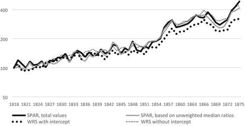
The original dataset consists of around 10,900 individual sales between the years 1818 and 1875. The total number of distinct properties (indentified by property name) is 5129. Out of this, 7758 transaction pairs could be constructed. This new dataset has 2811 distinct properties.

The WRS index constructed without an intercept displays a growth rate of 330 percent for the whole period, while the index with an intercept displays a growth rate of 215 percent. The intercept is estimated at 0.156. An interpretation is that each sale, on average, added 16 percent to the property value.

The SPAR method’ is used by Söderberg et al. (2014) for the period back to 1875, entailing that a ratio between the sales price and the tax assessment value is first constructed. Secondly, an index of the tax assessment value is reconstructed for the whole period under investigation. The tax assessment value only changes after a few years, which entails it is constant for periods of several years. Thirdly to arrive at a market price index, the ratio of the sale price, and tax assessment value is multiplied by the tax assessment value index.

To estimate the Housing Price Index in year t using the SPAR method, linking up to the Housing Price Index (HPI) from 1875 onwards, we use the following formula, where p_i,t is the price of object i in year t and T_i,X is the taxation value of object i in year X:(2) $HP{I}_t=HP{I}_{1875}\frac{{\sum }_i{p}_{i,t}}{{\sum }_i{T}_{i,X}}/\frac{{\sum }_j{p}_{j,1875}}{{\sum }_j{T}_{j,X}}$(2) Properties i are the ones sold in year t, and properties j are the ones sold in the year 1875, which entails that the estimated index may be spuriously affected by the composition of the sales in the actual year. For example, during some years larger properties may have been sold, which may not reflect the price level of the total stock.

An alternative method to estimate the Housing Price Index is based on the unweighted central measure (median, arithmetic average, geometric average, etc.), CM, of the ratios of market price to the taxation value:(3) $HP{I}_t=HP{I}_{1875}\mathrm{C}{\mathrm{M}}_{i,t}\left(\frac{p_{i,t}}{T_{i,X}}\right)/\mathrm{C}{\mathrm{M}}_{j,t}\left(\frac{p_{j,1875}}{T_{j,X}}\right)$(3) A problem with giving equal weight to each sale is that properties of lower value would then have a too large impact on the index. Giving equal weight may also be ad hoc since sometimes one sale consists of the sales of several properties. Using equal weights is also more sensitive to extreme values, when using just one taxation year, instead of applying several consecutive taxations. Therefore, when using formula (3), either the outliers should be deleted when using the arithmetic average, as is done in Söderberg et al. (2014), or an alternative central measure, such as the median or the geometric average, should be used, which are less sensitive to outliers. Although formula (2) is the appropriate formula to use if all properties would be sold every year, since they are not, various variants of formula (3) may be less sensitive for high valued properties being sold representing a large share of the total value sold in a given year.

For the period 1818–1875, the present study uses two different taxation values, 1861 and 1874, which generates two different nominal indices of property prices. Between 1861 and 1874, the taxation values increased substantially. However, the increase in the prices of properties was not uniform, some properties increased more than the average, probably due to building activities, while the value of other properties fell.

The difference between the two series in Figure 2 arises because the taxation values between 1861 and 1874 for the stock of sales in one year developed differently from the stock of sales in another year. A difference also occurs due to different coverage of the two indices, of different matching between sales prices and taxation values.

Figure 2. The nominal Housing Price Index 1818–1875 according to the SPAR method using two different taxation assessments, 1818 = 100.

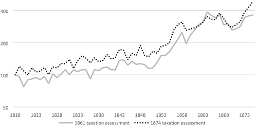
As can be seen from Figure 2 the two different series displayed almost the same average growth rate between 1818 and 1875. However, for the 1860s the two series display different levels. Using the taxation values of 1861 display higher property prices for the 1860s. The largest difference is for the year 1864. The ratio of the 1874 taxation value to the 1861 taxation value reached a top in this year, i.e. the sample of 1864 contained properties that tended to be valued exceptionally high in the 1874 taxation compared to the taxation of 1861. This condition may indicate that in 1864 more properties were sold that were affected by building activity. While according to the series using 1861 taxation values property prices on average grew by 99 percent between 1859 and 1864, according to the series using 1874 taxation values the growth was only 35 percent. Between 1864 and 1875 the opposite effect can be observed. Since it is difficult to judge which of the two indices is the most appropriate one, our final index is the geometric average of the two indices based on the two taxation values.

As Figure 1 shows, there are some differences between the SPAR index and the WRS index with an intercept. The initial SPAR index is similar to the WRS index without an intercept. The SPAR method may, therefore, catch some of the building activities rather than reflecting genuine price change. On the other hand, it is also possible that the WRS index with an intercept underestimates price changes due to the depreciation of the housing stock.

Figure 1 also compares the Housing Price Index when using formula (3), applying the median as the central measure. The alternative method yields a similar index as we had from formula (2).

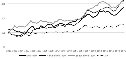
One way to determine the robustness of the indices is to compare the development of different geographical areas. Figure 3 presents the SPAR index for the Old Town (the parish of Nikolai), northern Stockholm (Östermalm, Norrmalm, and Kungsholmen) and southern Stockholm (Södermalm). The Old Town did not undergo the same transformation as the rest of the inner city, and the quality of building therefore probably remained unchanged. The comparison shows that the growth of the index in the Old Town was slower than in other parts of Stockholm. Prices in northern Stockholm tended to increase fast especially in the 1850s and 1870s, which, however, could reflect increases in land prices (an example is discussed below) rather the construction activity. The development in the Old Town is similar to the WRS index for the whole city using an intercept. All indices increased much faster than the Consumer Price Index.

Figure 3. The estimated nominal Housing Price Index of Stockholm 1818–1875 (1818 = 100), geometric 3-year moving average, in different geographical areas in Stockholm, using SPAR and the taxation values of 1874.

6. Long-run trends

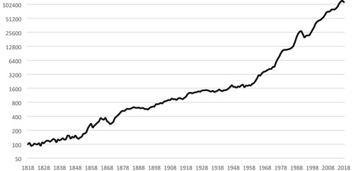
To analyze long-term trends, our series using SPAR is linked up to the series from 1875 to 2012 (Söderberg et al., 2014). The SPAR method is, therefore, applied for the whole period up to 1957. The index published in 2014 consists of several different series. In the period after 1957, the index only includes small houses, which better reflect the actual market prices of properties than apartment buildings, since the prices of the latter were suppressed due to rent regulation. The geopgrahical area of the index is expanded to reflect the growth of Stockholm. Up to 1957, our index covers the inner city, from 1957 to 1969 the City of Stockholm, in 1969–70 the urban area of Stockholm County, and from 1970 the Stockholm County. For the period 2012–2018, we extend the index using data on the value of small houses in Stockholm County from Svensk Mäklarstatistik (2018).

Figure 4 presents the nominal Housing Price Index, setting 1818 to 100. Between 1818 and 2018, the nominal index increased by 3.6 percent per year on average, while the inflation was on average 2.2 percent per year.

Figure 4. The nominal Housing Price Index 1818–2018, 1818 = 100.

In Figure 5 our index is deflated by the Consumer Price Index and by nominal GDP per capita, respectively. Although both deflators pertain to Sweden as a whole, property prices in Stockholm can be related to prices and incomes in other parts of the country as well. For example, if incomes fell in other parts of Sweden, fewer people would afford to move into Stockholm if property prices would remain the same.

Figure 5. Stockholm Housing prices, deflated by the CPI and the GDP per capita, 1818–2018, 1818 = 100. Source: Our data and Söderberg et al. (2014).

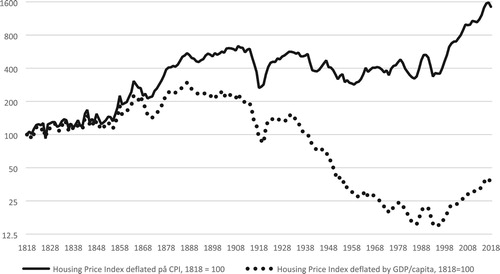
Our newly collected data for 1818–1874 indicates that Stockholm experienced another sharp growth in real prices during the second half of the nineteenth century, which complement the ‘hockey stick pattern’ in Knoll et al. (2017) with another hockey stick earlier in time. While they find almost no long-run real price growth in the first 90 years, but a sharp rise after 1960, we show that an increase started around 1855, accelerated in 1870–1886, and ended in 1887. In total, housing prices increased by 315 percent in real terms during this period, an increase only exceeded by our present-day increase from 1993 to 2017, when real prices increased by 370 percent. Using the WRS index with an intercept up to 1875 for robustness check entails that real prices between 1855 and 1887 only increased by 220 percent, which still was a substantial upturn.

The second ratio displayed in Figure 5 compares the index to the income levels (measured in GDP per capita). If the price of a property is divided into a structure and land component, technological development should cause a falling ratio if the structure component dominates price. However, if the land component is dominant, population pressure could cause the ratio to stagnate or even increase. A falling ratio should indicate that people afford more space, despite increasing real prices. Figure 5 shows that the level in the 1930s was about the same as in the 1820s. In 1858–1915 buying a property was most expensive, while after the 1930s, properties fell in value relative income, with a rebound after the 1990s. The long-term evolution of the residential property price deflated by GDP per capita is similar to the development of the wealth to income ratio (Waldenström, 2016).

The long-run movements in housing prices deflated by consumer prices and the GDP per capita can be related to long-run movements in economic and demographic conditions. Figure 6 displays the population of Stockholm municipality and the inner city, with somewhat different trajectories.

Figure 6. Population of Stockholm municipality and inner city 1800–2017. Source: Ström (2005) and www.scb.se

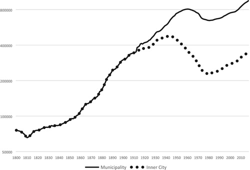
The real prices of residential properties were stagnating up to the mid-1850s. Stockholm had then been a modestly growing town for more than a century. The city had a population of around 75,000 in 1818 compared to around 60,000 in 1685.

The 1870s and 1880s were exceptional decades in Stockholm, of economic and demographic growth, which were accompanied by increases in real estate prices. The population increased by 20 percent (from 136,000 to 169,000 inhabitants) in the 1870s and by 46 percent (from 169000 to 246000 inhabitants) in the 1880s – which is the fastest relative increase in population ever in Stockholm (Johnson, 2017; Ström, 2005). Stockholm's population grew about half as much in relative terms between 1993 and 2017 as between 1855 and 1987 (Ahlberg, 1958; Johnson, 2017). Population growth most likely contributed to increases in land prices.

During the latter half of the nineteenth-century housing and real estate had become a lucrative business for capital investment. According to one source, the land north of Humlegården (in Östermalm) was worth only around 35 öre per square foot in 1878, but 1885 the value had risen to 5–6 kronor (Stockholms Intecknings Garanti Aktiebolag, 1919).

The new ‘hypoteksinstituten’, a sort of loan institute for real estate investment (which had been established in 1860), made investment possible for larger parts of the population. The house price deflated by GDP per capita reached a peak in 1887. Housing shortage was severe and solving it was not regarded as a task for the public service but for private investors who in the 1870s constructed 900 buildings and over 2000 buildings in the 1880s – which was more than had been built during the whole previous part of the nineteenth century. City planning and building laws were also introduced with ‘The Building and Fire Charter’ in 1874 which for instance stipulated that no new buildings were allowed to have more than five floors. However, these regulations did not have full legal status, which was known by many building contractors. The regulations were therefore often neglected in practice (Berglund, 2008). Their possible moderating effect on the expansion is thus uncertain.

After the mid-1880s there was, instead, a housing surplus as indicated by the decrease in the housing prices. Already in 1882, concerns of over-speculation had risen in political circles in Stockholm. When Hantverksbanken, a bank mainly involved in real estate loans, collapsed in 1885 a crisis spread with bankruptcies among builders and a decline in construction as a result (Hammarström, 1979, pp. 1860–1920).

Between 1885 and 1894 nominal prices decreased by 11 percent. Also, there were demands for specific professional qualifications for building contractors which since the freedom of trade reform in 1864 had been a profession without any requirements on formal education or qualifications; anybody could call themselves a building contractor between 1864 and 1888 (Råberg, 1976). From 1894 property prices started to increase again. Between 1894 and 1914 nominal prices increased by 78 percent, although real prices increased only 24 percent, given that inflation eroded some of the nominal gains. Also, both the ratio of wealth and financial debt to income increased all the way up to the First World War (Waldenström, 2016).

By 1900 the population in Stockholm had grown to 300,500 inhabitants. However, increases in population in different parts of Stockholm have often been followed by a local decline. The inner city, for instance – consisting of Nikolai, Klara, and Jakob, – grew between 1850 and 1880, but started to decrease afterward. The population in Johannes began to decrease in 1920, Södermalm in 1935 and Östermalm and Kungsholmen in 1945. However, Stockholm County as a whole (not displayed in Figure 6), including its expanding suburban areas, had a constantly growing population after 1850 (Ahlberg, 1958).

Housing prices continued to increase until 1909 when they reached a peak. In the long-term, it was followed by a negative price trend. The peak in real prices in 1909 was not surpassed until 2001. As Piketty and Zucman (2014) note, while before the First World War capital markets in the rich world ran unfettered, afterward a number of anti-capital policies depressed asset prices, causing the ratio of wealth to income to decline. Also, the price stagnation after approximately 1900, despite continuing rapid population increase in Stockholm inner city until the 1940s (in Stockholm municipality until the 1950s), can largely be explained by the innovations of infrastructure; with automobiles, busses and trains replacing horse and carriges. The so-called second industrial revolution (1870–1914) with the cumbustion engine as its main technological innovation revolutionalized travelling, commuting and infrastructure which of course increased the supply of land (by making it more accessible).

Between 1959 and 1981 the population of the municipality of Stockholm declined from 806,722 to 647,115. Between 1944 and 1980 the population of the inner city was more than halved, from 479,845 to 225,940 (Ström, 2005).

From 1957 we can separate prices of small houses from prices of apartment buildings. Interestingly, the two indices show different trends. While the real prices of apartment buildings fell, prices of small houses stagnated. The causes of the two different trends are not fully clarified but rent regulations and subsidises to rental apartment are likely explanations (Söderberg et al., 2014). Roine and Waldenström have studied the wealth effect of this divergence. They claim that decreasing inequality during this period can partly be explained by a combination of rising prices for small houses, a spread of ownership of small houses to a larger part of the population, and the decrease of apartment building prices (Roine & Waldenström, 2009).

In the 1960s, the ‘Miljonprogrammet’ (the Million programme) was launched, during which around 100,000 houses and apartments were constructed annually for ten years and a large part of the old building stock was demolished. The massive increase in supply had a major negative impact on real estate prices. Although this programme weakened the rationale for private wealth accumulation of housing, during the 1960s and 1970s, Stockholm was partly depopulated in favour of villas (‘egna hems-boenden’) in the suburbs.

The increase in real estate prices in the second half of the 1980s coincided with the deregulation of Swedish financial markets and an increase in private indebtedness (Ahnland, 2015). Similarly, the ratio of wealth and debt to income turned upwards (Waldenström, 2016). In 1985–90 real housing prices in Stockholm increased by 64 percent, reaching the highest level in half a century.

Since the early 1990s, there has been a rebound in the housing prices deflated by GDP per capita, indicating that housing has become less affordable. There is probably a combination of factors contributing to this development. The population has started to increase, while building activity has not increased to meet the demand. Nevertheless prices deflated by GDP per capita today are still at the same level as in the 1950s, and it is the low levels in the 1970s and 1980s, following the ‘Miljonprogrammet’ and the depopulation of the inner city, that could be viewed as exceptional.

7. Short term downturns in housing prices

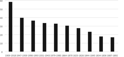
Figure 7 displays the ten largest downturns in nominal housing prices (during a period of maximum of 15 years), while Figure 8 displays the ten sharpest declines in real prices. A similar analysis could be made of upturns, which we leave out here. While declines in real prices by more than 25 percent occurred at several periods, declines of that magnitude were unusual for the nominal series; after 1875 it only happened once, in 1991–1993. Our new extended series shows that there was another nominal decline of that magnitude, occurring in 1864–1870; interestingly both periods were temporary dips during a longer upturn. Both declines in nominal prices also experienced sharp declines in real prices.

Figure 7. The ten sharpest falls in nominal housing prices in Stockholm 1818–2018 during a period of maximum 15 years that do not overlap.

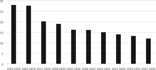
Figure 8. The ten sharpest falls in real housing prices in Stockholm 1818–2018 during a period of maximum 15 years that do not overlap.

The declines in nominal and real prices often followed crises in the real economy (Söderberg et al., 2014). During the pre-industrial era fluctuations in property prices were sometimes related to the agrarian cycles rather than the financial markets. The decrease in the late 1860s followed the harvest failures in 1865 and 1867, and the decrease in 1826 followed the harvest failure the same year. The declines in real prices during the world wars were accompanied by the sharpest declines in GDP during the twentieth century. However, some real economic crises were not followed by sharp declines in property prices. Some sharp real prices were the consequence of inflation rather than nominal decline.

With rising wealth and debt levels relative to income, Sweden became more prone to financial crises. The crisis of 1907, triggered by the San Francisco earthquake, had disastrous consequences for the Stockholm housing market. Construction came to a standstill and was worsened by labour market conflicts.

Turbulent trajectories, during and after the First World War, associated with high inflation or deflation, increased the volatility of real prices. The high inflation period during World War One was accompanied by a decline in real housing prices. Between 1909 and 1918 real prices dropped by a staggering 58 percent, the largest fall that we have recorded, but nominal prices increased by 9 percent. Since the deflation crisis at the beginning of the 1920s was not followed by a fall in nominal housing prices, the real house values rebounded sharply. In 1920–23 nominal housing prices increased by one percent; but since consumer prices dropped, real prices increased sharply. Nominal and real prices continued to increase during the 1920s, but the peak in real prices reached in 1931 was still 11 percent below the peak in 1909. Surprisingly, the 1929 depression and the Kruger crash did not lead to a severe drop. Both nominal and real prices decreased only by 9 percent between 1931 and 1936.

The largest fall in nominal housing prices, in the early 1990s, was accompanied by negative GDP growth during three consecutive years, the only time this occurred since the 1830s. In Stockholm nominal prices fell by 28 percent, the largest fall recorded since 1818.

Nominal declines tended to be counteracted by a floating exchange rate. Both the declines in the 1860s and 1990s occurred in periods of fixed exchange rates. During the 1860s, Sweden was on a silver standard, and the amount of silver in the riksdaler riksmynt was fixed. In 1873, when Sweden switched to the gold standard, the riksdaler riksmynt became the krona (Söderberg et al., 2014). Following the Great Depression, Sweden left the gold standard in 1931, which ameliorated the decline in property prices. In the early 1990s, the krona was fixed to the ECU. Since 1992 the krona is freely floating against the euro. The burst of the international housing bubble during the recent Great Recession did not impact on Stockholm housing prices. While the Swedish GDP fell by six percent in 2007–2009, nominal housing prices increased by three percent.

8. International comparison

Most long-run housing price indices start around 1900 or later and only a few stretches as far back as ours. Indices exist for the Norwegian towns of Oslo, Bergen, and Kristiansand (Eitrheim & Erlandsen, 2005, pp. 1819–1989). Eichholtz's Herengracht index is biannual covering the period of 1628–1973 (Eichholtz, 1997). Friggit presents data for Paris 1840–2015, a series that can be linked to Gaston Duons stretching from 1790 to 1840 (Friggit, 2009). The real housing price indices are depicted in Figure 9. Strikingly, all of them show a similar trend over the whole period.

Figure 9. Real Housing prices 1818–2017; Stockholm, Norway, Paris, and Herengracht. Indices in natural logarithms.

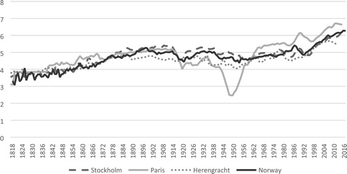
In Table 1, the growth rates for the different cities in different periods are compared. Herengracht sticks out in the period 1840–59 as the only town with a negative trend, which was generated by the price fall in the 1840s. In all our indices, growth is in general stronger in the early decades and fades out towards the end of the nineteenth century. Subsequently, housing prices entered some decades of stagnation, with turbulence around the two world wars, and started to pick up pace from around the 1960s. All countries have experienced booming housing prices the last 20 years.

Table 1. Mean percentage real housing price growth 1818–2017.

	Stockholm	Paris	Herengracht	Norway
1818–1839	6.1	23.8	6.5	10.0^a
1840–1859	8.5	15.1	−1.8	24.9
1860–1879	17.7	3.6	16.1	14.5
1880–1900	5.3	5.4	0.9	8.8
1900–1913	2.0	0.5	−3.6	−1.2
1914–1918	−15.3	−12.4	−2.1	−9.7
1919–1938	14.3	−3.0	−5.8	8.2
1939–1945	−5.0	−15.8	7.2	−6.6
1946–1959	−8.8	34.2	3.0	−2.2
1960–1979	10.3	24.2	12.9	5.8
1980–1999	3.1	3.4	8.1	11.3
2000–2017	17.2	13.6^b	0.0^c	13.6

^aThe index start 1819.

^bThe index end 2015.

^cThe index end 2012.

Most other longer housing price series only stretches back to around 1900. By extending the series to 1818 we show that the strong price growth that most advanced countries have experienced since the 1960s is not historically unique. Actually our index suggests that the indexes going back to 1900 start at the end of another period of steep growth, as is the case with the four examples presented here. Data collection for more towns would bring further light over this interesting issue.

As we can see in Figure 9 the evolution of the real house prices in 1818–2018 are similar in Stockholm, Paris, Herengracht and the cities of Norway, not least during the late nineteenth century and late twentieth early twenty-first-century boom in prices. The common trends in those cities could be explained by similar economic, geographical and institutional conditions. In Sweden and Norway the two long upturns in real prices were preceded by deregulation reforms, namely the freedom of trade reform in 1864 and credit deregulation reform in mid-1980s. The Netherlands and France introduced similar reforms during the same periods.

Sweden and Norway were in a political union between 1814 and 1905. The demographic expansion was more extreme in Norway's capital Oslo; between 1845 and 1890 its population increased 7-fold. Both in Sweden and Norway suburbanisation made the inner cities decrease radically between 1940 and 1980. Population growth became positive again in the late 1980s. Just like in Stockholm price regulations existed for all kinds of multifamily housing in Norway between 1940 and 1969, followed by some deregulations. As in Sweden, a municipality reform in the 1970s occurred in Norway, and credit deregulation took place in the 1980s. Important differences between Sweden and Norway exist of course. In 1940 rent control was introduced in Norway (Eitrheim & Erlandsen, 2004), but since 1982 it has been significantly reduced in Oslo, in contrast to Stockholm (Oust, 2017). Events like the 1916 Bergen fire, the invasion of the German army in World War Two and the discovery of oil reserves in the North Sea back in the late 1960s, making the country one of the richest in the world, are distinctive. Furthermore, Norway is not a member of the European Union.

Even though Amsterdam was a financial centre during the ‘Golden period’ of the seventeenth and eighteen centuries, by the nineteenth century the city was marked by military defeat and economic stagnation. The Netherlands lost Belgium in the revolt of 1830. In 1848 several liberal reforms were launched similar to the 1864 freedom of trade reform in Sweden. Just like in Stockholm, industrialisation was unleashed in Amsterdam in the late nineteenth century, accompanied by high population growth and housing price increases. Between 1849 and 1880 the population in Amsterdam increased from 224,000 to 320,000 (Eichholtz, 1997; Wielenga, 2015). Just as Sweden, Netherlands was and is a small open economy, belonging to the northern Europe-version of welfare capitalism (Esping-Andersen, 1990). Just like Sweden, Netherlands is part of the EU, but contrary to Sweden it has also adopted the Euro currency, which might explain why prices in Herengracht, but not in Stockholm, decreased during the financial crises of 2008.

Stockholm is least similar to Paris. During most of the period, 1818–2018, Paris has been either the largest or the second-largest city of Europe (Fierro, 1998). Already in the first half of the nineteenth century Paris was industrialised. Such differences may explain why the upturn in the late nineteenth century prices was not as distinct in Paris as in Stockholm, which started as one of the most impoverished towns in Europe in the nineteenth century. The revolts in 1848 and the Franco-Prussian war in 1870–71, when Paris was partly occupied, followed by the Paris Commune, might have contributed to the relatively modest growth in prices. Political events during the twentieth century, like the world wars, when Paris was occupied, naturally impacted on prices.

9. Conclusions

This study demonstrates the importance of having a longer time series of housing prices, which can put light on the recent upturn. Are we now experiencing a new housing bubble internationally, which will soon burst, or are the present levels of property prices sustainable in the long-run? Will the increase in the ratio of wealth to income continue in the future? May there be a reversal in the trend of increasing inequality? We do not know that now, but history can provide us with periods that are comparable. History can make us more open to several possible outcomes.

Reconstructing a historical housing price index is methodologically challenging. The main validity question is to what extent an index measures a constant quality over time, a problem that is aggravated in historical studies due to the limitation of the source material. We show that even if our index can be questioned, alternative estimates display similar results, although there are some differences. Further historical studies are necessary to consider quality changes. From an international perspective, Sweden has very rich sources that could be invaluable to studies on historical methodology. The main aim of the present study is not to present a final index, but to take the first step in analysing the development of historical housing prices for Sweden back to the pre-industrial era.

While the study of Knoll et al. (2017) indicates a ‘hockey stick’ development, with stagnation in real prices up to the 1960s, followed by a rapid increase, we show that the rise in the last decades had precedence in the second half of the nineteenth century. This rise was not immediately followed by a burst of a bubble back to the level before the rise, although there was a sharp decline in the 1860s, followed by a new rise. However, after the 1880s, there was a century of stagnant, or even slightly declining real prices. The real price in 1993 was 39 percent below the level in 1887. This period of secular decline was accompanied by a decline in the inner-city population during the post-war period.

The movement in real housing prices follows a similar pattern as the ratio of wealth to income. Through our historical analysis, we demonstrate how these long-term trends are related to institutional changes, which supports similar arguments made by Piketty and Zucman (2014). Extreme institutional chocks, such as wars, also depressed property prices. The two periods of market deregulation, in the third quarter of the nineteenth century and the late twentieth century, were accompanied by real capital gains, but also rising debt. During the pre-industrial period and the long period of increased regulation in the twentieth-century real housing prices were stagnating and the ratio of wealth to income declined. This pattern may suggest that more regulation and government intervention in the future most likely would curb real housing prices.

Disclosure statement

No potential conflict of interest was reported by the author(s).

Additional information

Funding

This paper has been written within a project financed by Torsten Söderbergs Stiftelse. For support we are also grateful to Sveriges Riksbank and Jan Wallanders och Tom Hedelius Stiftelse.

Notes

1 Swedish rents are today regulated through a collective bargaining system between landlords and tenants.

References

- Ahlberg, G. (1958). Stockholms Befolkningsutveckling Efter 1850. Monografier / Utgivna Av Stockholms Kommunalförvaltning, 0346-6035; 22:1. Stockholm.
- Ahnland, L. (2015). Private debt in Sweden in 1900–2013 and the risk of financial crisis. Scandinavian Economic History Review, 63(3), 302–323. doi: 10.1080/03585522.2015.1084946
- Bailey, M. J., Muth, R. F., & Nourse, H. O. (1963). A regression method for real estate price index construction. Journal of the American Statistical Association, 58(304), 933–942. doi: 10.1080/01621459.1963.10480679
- Berglund, K. (2008). Plan För Byggd Miljö: Förr Och Nu. In Bo Lundström & Ulf Jansson (Eds.), Bebyggelsehistorisk Tidskrift (Vol. 55, pp. 72–86). Uppsala: Bebyggelsehistorisk tidskrift.
- Bohlin, J. (2014). A price index for residential property in Göteborg, 1875–2010. In R. Edvinsson, T. Jacobson, & D. Waldenström (Eds.), Volume II: House prices, stock returns, national accounts, and the Riksbank balance sheet, 1620–2012 (pp. 26–62) Historical Monetary and Financial Statistics for Sweden 2. Stockholm: Ekerlids.
- Bonnet, O., Bono, P.-H., Chapelle, G., & Wasmer, É. (2014). Does housing capital contribute to inequality? A comment on thomas piketty’s capital in the 21st century. Sciences Po Economics Discussion Papers. Economics Department, Sciences Po and LIEPP.
- Bourassa, S. C. (2012). House price indexes. In S. J. Smith (Ed.), International encyclopedia of housing and home (pp. 247–251). San Diego: Elsevier. doi: 10.1016/B978-0-08-047163-1.00116-8
- Bourassa, S. C., Hoesli, M., & Sun, J. (2006). A simple alternative house price index method. Journal of Housing Economics, 15(1), 80–97. doi: 10.1016/j.jhe.2006.03.001
- Case, B., Pollakowski, H. O., & Wachter, S. M. (1991). On choosing among house price index methodologies. Real Estate Economics, 19(3), 286–307. doi: 10.1111/1540-6229.00554
- Case, K. E., & Shiller, R. J. (1987). Prices of single family homes since 1970: New indexes for four cities [Working Paper]. National Bureau of Economic Research. doi: 10.3386/w2393
- Deeter, K., Duffy, D., & Quinn, F. (2016). Dublin house prices: A history of booms and busts from 1708–1949. Journal of Statistical and Social Inquiry Society of Ireland, XLVI, 1–17.
- Eichholtz, P., Korevaar, M., & Lindenthal, T. (2019, July 11). 500 years of housing rents, quality and affordability [Paper presentation].
- Eichholtz, P. M. A. (1997). A long run house price index: The herengracht index, 1628–1973. Real Estate Economics, 25(2), 175–192. doi: 10.1111/1540-6229.00711
- Eitrheim, Ø., & Erlandsen, S. K. (2004). House price indices for Norway 1819–2003. In J. T. Klovland, Ø. Eitrheim, & J. F. Qvigstad (Eds.), Historical monetary statistics for Norway (pp. 349–376). Oslo: Norges Bank.
- Eitrheim, Ø., & Erlandsen, S. K. (2005). House prices in Norway, 1819–1989. Scandinavian Economic History Review, 53(3), 7–33. doi: 10.1080/03585522.2005.10414257
- Englund, P. (1993). Bostadsfinansieringen och penningpolitiken. In L. Werin (Ed.), Från räntereglering till inflationsnorm. Det finansiella systemet och Riksbankens politik 1945–1990 (pp. 155–193). SNS.
- Englund, P., Quigley, J. M., & Redfearn, C. L. (1999). The choice of methodology for computing housing price indexes: Comparisons of temporal aggregation and sample definition. The Journal of Real Estate Finance and Economics, 19(2), 91–112. doi: 10.1023/A:1007846404582
- Esping-Andersen, G. (1990). The three worlds of welfare capitalism. Cambridge: Polity.
- Eurostat. (2013). Handbook on residential property prices indices (RPPIs). Methodologies and Working Papers. European Commission.
- Fierro, A. (1998). Historical Dictionary of Paris. Lanham, MD: Scarecrow Press.
- Franzén, B., & Söderberg, J. (2018). Hus, Gårdar Och Gatubodar. Fastighetspriser i Stockholm Och Arboga 1300–1600. Historisk Tidskrift, 138(2), 2–29.
- Friggit, J. (2009). Le prix des logements sur longue période. Informations Sociales, 155(5), 26–33. Retrieved from https://www.cairn.info/revue-informations-sociales-2009-5-page-26.htm doi: 10.3917/inso.155.0026
- Gatzlaff, D. H., & Ling, D. C. (1994). Measuring changes in local house prices: An empirical investigation of alternative methodologies. Journal of Urban Economics, 35(2), 221–244. doi: 10.1006/juec.1994.1014
- Goetzmann, W. N., & Spiegel, M. (1995). Non-temporal components of residential real estate appreciation. The Review of Economics and Statistics, 77(1), 199–206. doi: 10.2307/2110007
- Hammarström, I. (1979). Urban growth and building fluctuations. Stockholm 1860–1920. In T. Hall (Ed.), Growth and transformation of the modern city: The Stockholm conference, September 1978, University of Stockholm (pp. 27–49). Stockholm: Swedish council for building research [Statens råd för byggnadsforskning]. Document / Swedish Council for Building Research, 0347-0962; 1979:17.
- Jacobsson, E. (1996). -Och Mödan Gav Sin Lön: Om Bostadspolitik Och Bostadskooperation i Stockholm 1870–1930. Stockholm: Univ., Ekonomisk-historiska institutionen.
- Johnson, A. (2017). Hela Stockholms Isaak Hirsch: Grosshandlare, Byggherre, donator 1843–1917.
- Jonung, L. (2008). Lessons from financial liberalisation in Scandinavia. Comparative Economic Studies, 50(4), 564–598. doi: 10.1057/ces.2008.34
- Knoll, K., Schularick, M., & Steger, T. (2017). No price like home: Global house prices, 1870–2012. American Economic Review, 107(2), 331–353. doi: 10.1257/aer.20150501
- Korevaar, M. (2018, December 8). The first housing bubble? House prices and turnover in Amsterdam, 1528–1810 [Paper].
- Lind, H., & Lundström, S. (2011). Kommersiella Fastigheter i Samhällsbyggandet. Stockholm: SNS förlag.
- Lindbeck, A. (2016). Hur Avveckla Hyreskontrollen? [Elektronisk Resurs]. In Ekonomisk Debatt. Ekonomisk Debatt. Retrieved from http://urn.kb.se/resolve?urn=urn:nbn:se:su:diva-140914
- Lyons, R. C. (2015). Measuring house prices in the long run: Insights from Dublin,1900–2015. Retrieved from http://eh.net/eha/wp-content/uploads/2015/05/Lyons.pdf
- Mark, J. H., & Goldberg, M. A. (1984). Alternative housing price indices: An evaluation. Real Estate Economics, 12(1), 30–49. doi: 10.1111/1540-6229.00309
- Mörner, G. (1997). Ljus Och Luft: Herman Ygberg – Stadsingenjör Och Stadsplanerare: 1844–1917. Stockholm: Stockholmia.
- Oust, A. (2017). The removal of rent control and its impact on search and mismatching costs: Evidence from Oslo. International Journal of Housing Policy, 1–21. doi: 10.1080/19491247.2017.1336876
- Perlinge, A. (2012). Bubblan Som Sprack. Byggboomen i Stockholm 1896–1908. Stockholm: Stockholmia förlag.
- Piketty, T., & Zucman, G. (2014). Capital is back: Wealth-income ratios in rich countries, 1700–2010. Quarterly Journal of Economics, 129(3), 1255–1310. doi: 10.1093/qje/qju018
- Råberg, M. (1976). En Framtid För 1800-Talets Stockholm?: Storstadens Framväxt Underindustrialismen: Aktuella Bevarande- Och Saneringsplaner. In Stadsvandringar (Vol. 1, pp. 7–27). Stockholm: Stockholms stadsmuseum.
- Raff, D., Wachter, S., & Yan, S. (2013). Real estate prices in Beijing, 1644 to 1840. Explorations in Economic History, 50(3), 368–386. doi: 10.1016/j.eeh.2012.10.003
- Rognlie, M. (2016). Deciphering the fall and rise in the net capital share: Accumulation or scarcity? Brookings Papers on Economic Activity, 2015(1), 1–69. doi: 10.1353/eca.2016.0002
- Roine, J., & Waldenström, D. (2009). Wealth concentration over the path of development: Sweden, 1873–2006. Scandinavian Journal of Economics, 111(1), 151–187. doi: 10.1111/j.1467-9442.2008.01558.x
- Sheiban, H. (2002). Den Ekonomiska Staden: Stadsplanering i Stockholm under Senare Hälften Av 1800-Talet. Arkiv Avhandlingsserie, 0347-4909; 56. Lund: Arkiv.
- Shiller, R. J. (2016). Irrational exuberance. Princeton: Princeton University Press.
- Söderberg, J., Blöndal, S., & Edvinsson, R. (2014). A price index for residential property in Stockholm, 1875–2011. In R. Edvinsson, T. Jacobson, & D. Waldenström (Eds.), Historical monetary and financial statistics for Sweden, vol. 2: House prices, stock returns, national accounts and the Riksbank balance sheet 1620–2012 (pp. 63–100). Stockholm: Sveriges Riksbank and Ekerlids.
- Stockholms intecknings garanti aktiebolag (1919). “Stockholms intecknings garanti aktiebolag 1869–1919.” Stockholm.
- Ström, S. (2005). “Befolkningen i Stockholm 1252–2005: Från 1721 Enligt Stadens Statistiska Årsböcker.” Stockholms stad, Utrednings- och statistikkontoret. Stockholm.
- Waldenström, D. (2015). Swedish National Wealth Database (SNWD): Appendix [Working Paper]. Uppsala University.
- Waldenström, D. (2016). The national wealth of Sweden, 1810–2014. Scandinavian Economic History Review, 64(1), 36–54. doi: 10.1080/03585522.2015.1132759
- Wielenga, F. (2015). A history of the Netherlands. London: Bloomsbury Publishing.
- Official publications
Physical sources
- Stockholms magistrat- och rådhusrätt, A 6 a Lagfarts-, uppbuds-, protokoll, vol. 71–85.
- Stockholms magistrat- och rådhusrätt, D4, Förteckning över uppbundna fastigheter, vol. 1–2.
- Stockholms rådhusrätt, Avdelning 1, A 1 A Lagfartsprotokoll, vol. 1–12.
- Stockholms Stad (1856–1974). Stockholms Adresskalender.
Electronic sources
- Svensk Mäklarstatistik. (2018).
- Statistiska centralbyrån (2018). https://www.scb.se/
- Stockholms stad (2018). http://statistik.stockholm.se
- Stockholmskällan (2018). http://www.stockholmskallan.se