Scraping the bottom of the barrel? Evidence on social mobility and internal migration from rural areas in nineteenth-century Norway

ABSTRACT

We aim to answer whether expected occupational gains motivated rural-urban and rural-rural migration in nineteenth-century Norway. Human capital theory indicates that the higher expected gains, the more prone an individual will be to migrate. We use a micro-level data set of over 42,000 rural sons linked to their fathers based on 1865 and 1900 Norwegian censuses and employ a switching endogenous regression model controlling for the endogeneity of migration decisions. Our main finding is that the effect of expected occupational gain on the probability of rural-urban migration differs according to the rural sons’ destination and parental occupational status: the sons from low status families were migrating motivated by expected occupational advancement. Sons from families with higher occupational status were motivated by expected occupational gains only in the case of rural-urban migration.

KEYWORDS:

• Regional migration
• migration decision
• expected occupational gains
• self-selection

JEL CODES:

• R23
• N33
• N93

1. Introduction

The population in Norway increased from 1.7 million in 1865 to over 2.2 million in 1900. The rural population increased in the same period, from 1.4 to 1.6 million (Statistisk Sentralbyrå, 1969). Although many people moved from rural to urban areas, consistent with what we would expect in an era of industrial and urban revolutions, a substantial number of internal migrants moved to other rural areas (Østrem, 2014). We may ask: Who went where, who stayed, what background did they all have, and, even more importantly, why did they choose to stay or move?

To shed light on these questions and the surprising stability of the rural population, historians and other scholars have interestingly pointed to the importance of attractive rural opportunities compared to urban opportunities. This contrasts with what seems to have been the case in other parts of Europe (Brox, 2013; Gjerdåker, 1981). These suggestions are consistent with a human capital approach to migration (Sjaastad, 1962), positing that rural individuals would prefer moving to another rural destination rather than staying provided the expected benefits exceed the costs. The argument has been substantiated through historical microstudies and anecdotal evidence, but these narratives’ generality beyond the local context is not clear. Before taking on this task, we may ask ourselves if there is any reason beyond pure curiosity. One answer is that we need to understand what was going on in the rural communities in this period. This is so we may be cognisant of the great social and economic transformations that led to the egalitarian society often associated with the Nordic model (see, e.g. Brox, 2000).

We take advantage of relatively recently available digitised and linked full count census data from 1865 and 1900, applying modern microeconometric techniques to control for potentially confounding factors and selection bias. The data allow us to trace sons from rural families over time and between geographical locations. More precisely, we ask whether sons from rural families moved based on expected occupational gains. Given the relative stability of the rural population overall, we consider rural-rural and rural-urban migration as alternatives to staying and allow for potential differences in selection bias and expected occupational advancement between these two outside options. We also look at how socioeconomic backgrounds influenced migration decisions through its effect on opportunities in the source municipality and the destination. The third option also available during this period was emigration to the New World. Although we concentrate on the two outside options open through internal migration, we also control for emigration in the empirical analysis.

The same source of data (in combination with other data) has been used in some recent studies focusing on emigration (Abramitzky, Boustan, & Eriksson, 2012; Abramitzky, Boustan, & Eriksson, 2013) and intergenerational social mobility (Modalsli, 2017). Approaches resembling ours, based on historical data, can be found in Long (2005) and Stewart (2006). More specifically, our study uses the endogenous switching regression (ESR) model – an extension of the well-known Heckman sample selection technique (Heckman, 1974). The ESR model corrects for sample selection bias and is sufficiently flexible to allow for endogenous self-selection related to migration. This approach is rather demanding in terms of sample size, but this is not a problem as our study includes more than 42,000 individuals.

We find that most rural sons chose to stay in their home municipalities. Cotters’ sons moved more than farmers’ sons to both rural and urban destinations. We find that expected occupational advancement was a stronger motive for migration for sons of low social status families. Migrants were not random samples. Cotters’ sons moving were negatively selected (‘the bottom of the barrel’), whereas farmers’ sons were positively selected (‘the cream of the crop’).

Abramitzky et al. (2013) and Modalsli (2017) also speak to rural-rural and rural-urban internal migration in Norway in the same period based on the same data source. However, we are addressing different questions. Abramitzky et al. (2013) study migration outcomes explained by proximate causes at the origin. We focus on labour market opportunities as a fundamental cause for the migration choice, measured by expected occupational gains estimated at the destination as well as the origin. Moreover, we account for selection bias, ignored by Abramitzky et al. (2013). Modalsli (2017) focuses on intergenerational social mobility but touches en passant on issues relevant for us from a very different methodological angle. More specifically, he suggests that internal migrants were negatively selected, consistent with what we find for rural sons from low-status families. However, we also find that this is not the case for rural sons from high-status families. These matters will be discussed in much more detail later.

The rest of this article is organised as follows. The details on the data and the matching procedure linking the 1865 and 1900 censuses are presented in Section 2. The Norwegian historical context is discussed in Section 3. The statistical model is presented in Section 4, and the estimation procedure is described in Section 5. The results are presented in Section 6, followed by a concluding discussion in Section 7.

2. Data and matching

We use 1865 and 1900 Norwegian census data sets linked by the Norwegian Historical Data Centre (NHDC) and provided by the North Atlantic Population Project (NAPP) (Minnesota Population Center, 2020). Both censuses are complete counts of the entire Norwegian population.

The NHDC linking procedure is based on the Integrated Public Use Microdata Series (IPUMS) linked representative samples approach (Goeken, Huynh, Lynch, & Vick, 2011; Ruggles, Roberts, Sarkar, & Sobek, 2011; Ruggles, Fitch, & Roberts, 2018). The procedure relies on four variables that would (theoretically) be stable over time: birth year, municipality of birth, given name, and surname. The method starts by identifying a set of potential matches for each record and then creates age and name similarity scores for each pair of potential links.

The linked sets were constructed to match a census sample to a complete census enumeration. In the linking process, census records were only compared if they exactly matched the municipality of birth. On the other hand, the age and name variables were allowed to vary slightly. The variation in age was allowed to be up to three years higher or lower than expected. Due to patronyms, NHDC truncated surnames prior to the patronymic suffix (for example Jespersen to Jesper) to minimise inconsistencies in the spelling of suffixes. The individuals in the linked sample had to match on first, middle, and surname. The linked male files represent all men (with information about their households) in Norway in both census years. To identify potential links, NHDC used scripts that contained the Jaro-Winkler name similarity algorithm.¹ From this linked set, we then constructed our data set where sons were linked to their fathers.

Table 1 shows the match rate for our sample. To reduce so-called life cycle bias (see for example, Bhashkar & Miguel, 2015), we include only sons aged 35–70 years in 1900 in our sample (whose fathers in 1865 were also between 35–70 years). First, we have to estimate the matchable population: In the 1900 census, we initially found 263,038 males between 35 and 70 born in Norway's rural municipalities. The second column shows that 83,690 of the rural sons aged 0–35 in 1865 were still residing in Norway in 1900. The match rate calculated this way is 31.8%. We know the identity of the father for 50,610 rural sons in this age group in 1865.

Table 1. Match rates.

Estimated matchable population in 1900	Share found in 1865	The share of the matched population that were registered as sons, and for which we have the identity of the father in 1865	Matched population	Father's age 35–70 and both father and son have HISCAM status	Final sample
263,038	31.8% (83,690)	60.4%	50,610	84.0%	42,219

Our study's matched population is comparable with other studies using data from the Norwegian 1865 and 1900 censuses. Abramitzky et al. (2013) use the iterative matching strategy by Ferrie (1996) and achieve a match rate of 26%. In his seminal paper on intergenerational mobility in Norway, Modalsli (2017) reports a match rate of 36.9%. Regarding other linked data sets of similar scope as those above, Long and Ferrie (2013) have match rates of 20% for Britain and 22% for the U.S. in the period 1850/51–1880/81. The same British linked data set with the same linkage is also used in Long (2005) and Long (2013).

We also check and confirm that our matched sample is representative of the population (see Table A1 in the Appendix). There is a slight over-representation of older sons and sons that lived in their municipality of birth in 1865. This likely occurs because the linked data over-represent established people, especially on farms (Thorvaldsen, 2011).

We include only sons defined as biological sons in our data set. More importantly, we also observe the characteristics of the childhood households in 1865. Our analysable data set contains information on occupational status for 42,219 sons in 1900, who in 1865 resided in their father's household in a rural municipality and whose father had a known occupation. By 1900, 5,355 of these sons had moved to urban municipalities, and 6,790 had migrated to rural municipalities.

Our data set has some limitations, e.g. it does not include information about overseas migration. Instead of urban migration, migration overseas may have been a real alternative for many rural residents. In addition, urban migration could have been only a first step of a migration process whereby rural residents first went to cities within Norway and then to destinations overseas. The selection process of emigration is an important part of the story but cannot be addressed with these data. However, we do have information on emigration rates at the municipal level that can be used as control variables. Neither are we able to identify return migration, only permanent moves. Those rural sons who returned to their municipality of origin before 1900 are registered as rural persisters. It is not possible to address this limitation in our data.²

We define rural-urban migration as a movement from a rural childhood municipality to an urban municipality between 1865 and 1900. Similarly, rural-rural migration is a movement from a rural childhood municipality to another rural municipality. To correct for municipality splits and amalgamations in Norway in this period, we also used 1865 municipality borders for municipalities in 1900. To categorise municipalities, we use the same classification as Norwegian authorities used in the 1800s. Urban municipalities were classified as either administrative cities (kjøpsted) or cities with more limited city rights (ladested). A kjøpsted was a town with privileges that gave its citizens a monopoly on trade and other industries. A ladested was historically subordinated to the nearest kjøpsted. A ladested generally had the same commercial rights as a kjøpsted but fewer public services and was considered a ‘candidate city’ with lower status and prestige than a kjøpsted.

Our occupational data are based on the HISCAM scale (Lambert, Zijdeman, Van Leeuwen, Maas, & Prandy, 2013). This scale combines HISCO (see Van Leeuwen, Maas, & Miles, 2004) and data on social interaction. The scale is developed by using patterns of intergenerational occupational connections. Lambert et al. (2013) used marriage records and similar data for seven (now developed) economies in the period 1800–1890 to gather the occupations for pairs of persons with a social connection (a so-called method of ‘social interaction distance’). In the absence of a Norwegian version of HISCAM, we use the Swedish version, as Norway was in union with Sweden in the study period. Our study uses all available information by applying the HISCAM scale, without sacrificing either tractability or standardisation. This means that we have an approximate continuous scale (417 different occupational categories in 1900). Using this continuous scale allows for flexibility concerning modelling and provides more intuitive estimates than using HISCO.

In our analysis, we divide our sample into two groups according to the father's occupational status in 1865, as we know that parental wealth and resources affect migration decisions (Abramitzky et al., 2013; McKenzie & Rapoport, 2010). In Norway, the social groups in rural areas that were clearly worse off in wealth and resources were cotters and lower social groups (such as unskilled workers and day labourers) (Semmingsen, 1977). Therefore, to study whether the role of expected occupational advancement in migration decisions differed by socioeconomic background, we split our sample into households with a HISCAM code in 1865 equal to or lower than 52.18 (cotters with land) and households with a HISCAM code higher than 52.18. We call the groups ‘lower occupational status’ and ‘higher occupational status’, respectively.

3. Description of the sample

Regarding the second half of the nineteenth century, Norwegian historians talk about two major domestic migration flows (Gjerdåker, 1981; Helle, 2006). One flow went from rural areas to towns and cities. Often, it was an instance of short-distance movement to a nearby centre. The large cities, especially the capital Christiania, attracted immigrants from a larger area and parts of the entire country. People also often came from far away to new industrial sites, such as Rjukan or Odda. The second type of migration took place regionally between rural municipalities. Because Northern Norway had vacant land and many fish to offer, a significant number moved north from more or less overpopulated areas in southern Norway (e.g. Voss, Gudbrandsdalen, Østerdalen, and Trøndelag).

By far, most rural-urban migrants moved to a town or city within their own province (see Table 2).

Table 2. Origin and destination provinces for rural-to-urban migrants. Row = 100%.

		Destination
		Capital area	Eastern inland	South-east Norway	South-west Norway	Western Norway	Central Norway	Northern Norway	N
Origin	Capital area	89%	1%	7%	2%	1%	1%	0%	872
	Eastern inland	63%	20%	10%	1%	1%	2%	2%	555
	South-east Norway	36%	0%	62%	1%	1%	0%	0%	1948
	South-west Norway	8%	0%	3%	85%	3%	0%	0%	688
	Western Norway	6%	0%	2%	9%	78%	3%	2%	763
	Central Norway	14%	2%	3%	2%	10%	59%	10%	313
	Northern Norway	16%	1%	3%	2%	12%	9%	57%	316
	N	2019	135	1372	712	705	266	246	5455

The same goes for the rural-rural migrants. Intraprovincial moves were even more common in this category (see Table 3). High long-distance migration costs were obviously very important in terms of mobility decisions. Transportation by sea along the coast could be the only practical option in many long-distance migration cases. However, to the extent that interprovincial moves took place, it is apparent from Tables 2 and 3 that the capital area was the most important destination for rural-urban movers, and most of them arrived from nearby provinces in eastern inland and southeastern Norway. We also observe that the eastern inland area is the only province where intraprovincial rural-urban moves were less important than interprovincial moves. Moreover, more than 60 per cent of the rural-urban migration from the eastern inland area went to the capital area. Interestingly, Table 3 shows that long-distance rural-rural migration to Northern Norway was widespread, not only from neighbouring Central Norway but also from the more distant provinces of Western Norway and inland Eastern Norway. Northern Norway was often an alternative to emigration abroad for poor households (Østrem, 2014); as in America, the province still had unexploited resources and thinly settled areas with vacant land.

Table 3. Origin and destination provinces for rural-to-rural migrants. Row = 100%.

	Destination
	Capital area	Eastern inland	South-east Norway	South-west Norway	Western Norway	Central Norway	Northern Norway	N
Capital area	69%	7%	21%	1%	1%	1%	1%	496
Eastern inland	16%	62%	10%	1%	2%	3%	7%	875
South-east Norway	10%	2%	84%	3%	0%	0%	1%	1846
South-west Norway	1%	1%	4%	90%	4%	0%	1%	852
Western Norway	1%	2%	2%	4%	73%	5%	14%	1174
Central Norway	1%	2%	1%	0%	4%	67%	25%	577
Northern Norway	1%	1%	1%	0%	1%	2%	95%	1086
N	686	661	1809	884	959	493	1414	6906

Most rural-rural and rural-urban migration was directed to nearby municipalities, and 80 per cent of migration in both categories went to destinations under 100 kilometres from the origin municipality (see Table 4).

Table 4. Distribution of rural-rural and rural-urban migration flows by distance.

Rural-rural migration	%	Rural-urban migration	%
Less than 50 km	62%	Less than 50 km	55%
50–100 km	18%	50–100 km	23%
100–500 km	15%	100–500 km	18%
500–1000 km	4%	500–1000 km	3%
Above 1000 km	1%	Above 1000 km	1%
Average distance	104 km	Average distance	101 km

The municipality characteristics show that rural-urban migration often took place in the near vicinity of urban municipalities, see Table A2 in Appendix. The average distance from home municipality to the nearest urban municipality for urban migrants was 26 km, while it was over 20 km longer for those who chose to stay in their municipality of origin. Rural-urban migration was most likely for rural sons near Christiania. Almost one-third of the rural sons from this area moved to urban municipalities. Christiania was also the main destination of rural-urban migration: 37 per cent of migration to urban areas went to the capital.

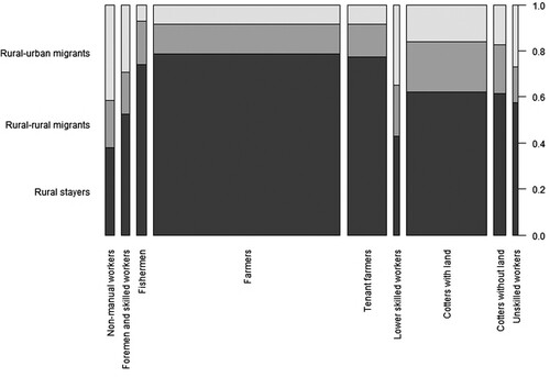
Who moved, who stayed and what backgrounds did they have? There seems to be a consensus among historians about the following pattern regarding rural-urban migration such that people from the cotter and lower classes migrated more frequently than farmers. Real estate binds. Similarly, people from families with lower occupational status and sons without allodial rights made up most rural-rural migrants (Gjerdåker, 1981). In our sample, we observe this pattern very clearly (see the spine plot in Figure 1). The vertical extent shows the fraction of migrant and non-migrant sons given fathers’ occupational status in 1865.³ The horizontal extent of the bars shows the fraction of fathers in different occupational classes. The areas of the ‘tiles’ represent the total sons by migration category and father's occupational status. It is clear that the sons of farmers had the lowest propensity to move. The second-largest group, sons of cotters, had a much higher propensity to migrate on average, not only to urban areas but also to other rural municipalities. Sons of fathers from the two highest classes, together with lower-skilled workers, had the highest probability of migrating to urban municipalities.

Figure 1. Shares of non-migrants, rural migrants and urban migrants by father's social status.

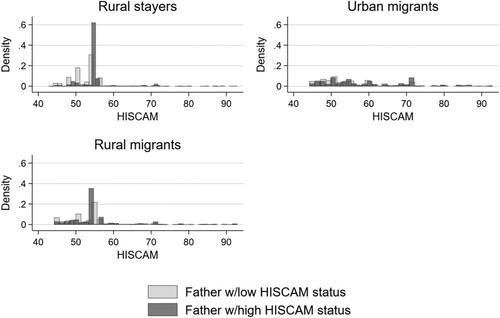
Family background also affected how well sons fared in the labour market. Figure 2 shows sons’ occupational HISCAM status in 1900 according to their migration status. We see that the occupational distribution of migrants from households of low occupational status is more left-skewed than for migrant sons coming from households of higher occupational status. This is also the case for stayers. We can also see that the distribution of occupations is rather similar for rural migrants and rural stayers. This means that rural migrants worked in the same occupations as rural stayers to a rather large extent.

Figure 2. Distribution of sons’ occupational HISCAM statuses in 1900 by their migration status and parental occupational status.

Table 5 gives a more detailed view of which occupations migrants held in 1900. The top five occupations are presented for each group. 36 per cent of sons from low-status families who migrated to another rural municipality owned their farms by 1900. For cotters’ sons, becoming a farmer was a big step up on the status ladder. 43 per cent of sons from higher occupational status families migrating to another rural municipality became farmers there. Interestingly, the top five occupations for rural-rural migrants are rather similar, possibly indicating that it was not expected labour market advancement that motivated farmers’ sons to move to rural municipalities. When we look at the most frequent occupations in 1900 for sons that migrated to urban municipalities, there are clear differences. The most frequent urban occupation for high-status family sons was working as a proprietor within a wholesale or retail enterprise (HISCAM status 61.69). In contrast, carpentry was the most common occupation for sons from lower socioeconomic backgrounds (HISCAM status 51.99). Interestingly, many higher-status sons became shipmasters (HISCAM status 71.67), while lower-status craft occupations dominated the top five job descriptions for lower-status sons in urban municipalities. Looking at the occupations’ names, it is also clear that many urban migrants worked in the old-fashioned craft industry rather than the ‘modern’ industries of the time, such as the textile and metal industries. Many historians (Bull, 1966; Myhre, 1977) have written about this tendency. Rural-urban migrants often took advantage of their work experience from adolescence, labouring in occupations where they could use the skills they learned in rural areas after moving to urban municipalities.

Table 5. Top 5 son’s occupations and their shares in 1900 by father’s lower and higher occupational status. HISCAM score in parentheses. Rural-rural migrants and rural-urban migrants.

Rural-rural migrants				Rural-urban migrants
Father's occupation lower status in 1865 (average HISCAM score 49.5)		Father's occupation higher status in 1865 (average HISCAM score: 55.8)		Father's occupation lower status in 1865 (average HISCAM score: 49.2)		Father's occupation higher status in 1865 (average HISCAM score: 57.3)
Son's top 5 occupations 1900 (average HISCAM score: 53.1)	%	Son's top 5 occupations 1900 (average HISCAM score: 55.8)	%	Son's top 5 occupations 1900 (average HISCAM score: 55.0)	%	Son's top 5 occupations 1900 (average HISCAM score: 59.3)	%
Farmer (54.5)	36	Farmer (54.5)	42	Carpenter (51.99)	6	Working Proprietor (61.69)	7
Fisherman (56.05)	8	Fisherman (56.05)	8	Shoemaker (50.0)	5	Carpenter (51.99)	5
Cotter (50.18)	5	Farm worker (49.51)	4	Sawyer (44.2)	4	Ship's Master (71.67)	5
Sawyer (44.2)	4	Carpenter (51.99)	3	Working proprietor (61.69)	4	Seaman (48.13)	3
Farm worker (49.51)	4	Cotter (50.18)	3	Day-labourer (45.83)	4	Fisherman (56.05)	3

Our main focus is to analyse how expected occupational gains motivated rural-urban and rural-rural migration in nineteenth-century Norway. According to Norwegian historians, future job prospects seem to have affected individuals’ migration decisions. Myhre (1981) writes about the labour market expectations of rural migrants moving to Christiania (our translation): ‘But our predecessors did not go out helpless or at random. They obviously had a notion of winning something by moving. There was also something that pulled them. At least they had heard that in the city, there were many who got jobs. Most of the migrants did not have a specific job or position in sight when they arrived. They came with hopes of profit and better livelihoods. Even less often had they acquired a residence in advance. Nevertheless, they knew that the city offered opportunities for those who were lucky or skilled and that the obstacles were fewer than where they came from’ (Myhre, 1981, p. 139). Gjerdåker (1981, p. 45 ) describes the role of rural job opportunities for a cotter's son (our translation): ‘When they then got to know about better conditions elsewhere than what they were used to on their small farm – and when they could trust that what they heard was not loose talk – then they gladly took the travel stick out and sometimes left to go far off’. Therefore, people were seeking new and improved life chances and the opportunity for a better job. Moving from a rural area in nineteenth-century Norway was not done as a randomly assigned adventure; an individual's expectations concerning labour market opportunities surely influenced their decision about whether to move or not. We aim to answer quantitatively whether these expected labour market opportunities motivated rural-urban and rural-rural migration.

4. The model

To determine whether people moved to take advantage of opportunities for expected occupational advancement, we need a model flexible enough to study the expected gains and mobility decisions, as well as the relationship between them.

Furthermore, it is important that our model takes censoring and selection bias into account. The issue of selection bias in economics was first raised by James Heckman (1974) in his analysis of women's wages and labour supply, building on Roy's (1951) work on self-selection. Yezer and Thurston (1976) brought the selectivity problem into migration research when they noticed that calculating only the returns of migration for successful migrants would lead to an upward bias in the estimates. The problem arises as the returns of migration for non-migrants are not reported, and we do not know what their prospective returns would have been if they had moved. Using only migrants’ observed returns in the analysis gives biased estimates of the population parameters.

The proposed solution to the selectivity issue by Heckman (1974) was an endogenous switching regression (ESR) model. The ESR model extends upon the tobit model by James Tobin (1958) and introduces a simultaneous equation system. In Heckman's example, individuals from different regimes (working and non-working women) can be included. Different parameters in the model affect the probability of an individual selecting into a certain group.

The ESR model was first applied in migration research by Nakosteen and Zimmer (1980) to estimate and adjust for nonobservable information. Heckman (1974, 1976, 1979) developed a two-step approach to estimate hypothetical earnings at the origin for movers and the destination for nonmovers while controlling for the selectivity process.

The two-step approach involves first predicting the probability that a certain individual self-selects into the different regimes. The estimates from the first step are then used as exogenous variables in the second step, where the outcome of selecting a certain regime is predicted, to account for the selection process. Given the long tradition of using this migration research approach, this model is a natural choice for our analysis. However, contrary to Heckman, we follow Nakosteen and Zimmer (1980) and perform the two steps simultaneously by applying full information maximum likelihood (FIML). Simultaneously, estimating the probit criterion and the occupational status regression equation will yield consistent standard errors and is more efficient.

The ESR model estimated with FIML allows us to answer our research question when facing the same censoring and selectivity issues as Heckman (1974) and others, giving us consistent and unbiased estimates.⁴

We apply our model with two regimes: moving and staying. Introducing some notation for making it more precise, the model is written, (1) ${\mathrm{M}}_i=1\mathrm{i}\mathrm{f}{\gamma }_1^{\mathrm{\prime }}{Z}_i+{\gamma }_2^{\mathrm{\prime }}\left(y_{1i}-y_{0i}\right)+u_i\ge 0$(1) (2) ${\mathrm{M}}_i=0\mathrm{i}\mathrm{f}{\gamma }_1^{\mathrm{\prime }}{Z}_i+{\gamma }_2^{\mathrm{\prime }}\left(y_{1i}-y_{0i}\right)+u_i<0$(2) (3) $y_{1i}={\text{β}}_1^{\mathrm{\prime }}{X}_{1i}+e_{1i}\mathrm{i}\mathrm{f}{M}_i=1$(3) (4) $y_{0i}={\text{β}}_0^{\mathrm{\prime }}{X}_{0i}+e_{0i}\mathrm{i}\mathrm{f}{M}_i=0.$(4)

Here, the dependent variables $y_{1i}$ and $y_{0i}$ represent the expected occupational HISCAM status if an individual moves or stays, respectively. As the possible occupational status in the counterfactual cases – for movers in rural origin areas and rural stayers in destination areas – is not directly observable, they are estimated in the model.

The identifiers $X_{1i}$ and $X_{0i}$ are vectors of variables explaining an individual's occupational status in cases where they move or stay, respectively. They include household, individual and municipal variables expected to affect opportunities in the labour market. The error terms $e_{1i}$ and $e_{0i}$ are measures of unobservable characteristics such as a person's energy or general abilities.

The identifier $M_i$ is the migration decision (1 = moving, 0 = staying). We estimate the selectivity-corrected status that individuals could have earned as movers and stayers, thus $\left(y_{1i}-y_{0i}\right)$ represents the expected difference in occupational status between the origin and destination municipalities, i.e. the expected gains (or losses) from moving. These values are not known beforehand and are estimated. The decision to migrate will thus depend on the expected occupational gains of moving, $y_{1i}-y_{0i}$, in addition to a vector $Z$ of other factors affecting the migration decision. The vector $Z$ includes measures we believe affect the costs of moving to an urban area. If the structural parameter ${\gamma }_2^{\mathrm{\prime }}$ is a positive and statistically significant parameter, movements of migrants in Norway would have taken place according to a process of maximising expected occupational gains, consistent with human capital theory.

The error terms in the migration decision equation $u_i$ can be interpreted as unobservable characteristics affecting the probability of moving, for example, the propensity to take risks or be ambitious. The error terms $e_{1i}$, $e_{0i}$ and $u_i$ are assumed to be jointly normally distributed. We use the correlation between the error terms in the status equations and the migration decision equation ${\rho }_1$ to determine the presence and direction of migration selectivity in determining occupational status outcomes.

5. Estimation of the model

We first look at the variables expected to affect sons’ opportunities in the labour market (the elements of X in equations (3) and (4)). The determinants of the son’s occupational status in 1900 include his parents’ HISCAM status, whether they owned land or a business, and whether the father lived in his municipality of birth. Individual determinants further include the son's age, whether the individual was the eldest son in the household, and the number of siblings. All explanatory variables are from the 1865 census and thus before the migration decision (see Table 6 for the variable definitions). Table A2 in Appendix shows descriptive statistics for rural-urban migrants, rural-rural migrants and rural stayers.

Table 6. A summary of determinants of occupational status and migration equations.

Variable	Definition	Occupational status equation $X$	Migration equation $Z$
Household and individual characteristics
Father's HISCAM status	HISCAM status of son's father in 1865	Yes	No
Number of servants	Number of servants in the household in 1865	Yes	Yes
Son's age	Son's age in years in 1865	Yes	Yes
Number of siblings	Number of son's homeliving siblings in 1865	Yes	No
Eldest son	Dummy variable = 1 if son is the eldest son among sons in the household in 1865	Yes	No
Father owns land or business	Dummy variable = 1 if household owned land or a business in 1865	Yes	No
Father in the municipality of birth	Dummy variable = 1 if father was born in the same municipality where the family resided in 1865	Yes	No
Son in the municipality of birth	Dummy variable = 1 if son was born in the same municipality where the family resided in 1865	No	Yes
Expected occupational gains of migration, $\left(y_{1i}^{\ast }-y_{0i}^{\ast }\right)$	Expected occupational differential between destination and origin municipality	No	Yes
Municipality (of origin) characteristics
High share of emigrants	Dummy variable = 1 if municipality lost over median share of its population as emigrants in 1865	No	Yes
km to nearest city	Euclidean distance from a rural municipality's centroid to a nearest urban municipality's centroid	Yes	Yes
Cities/towns within 100 km	Number of urban municipality centroids within 100 km from a rural municipality's centroid	Yes	Yes
Share in secondary sector	Share of employment in a municipality working in secondary sector	Yes	Yes
Province (of origin) characteristics
Provincial dummies	Dummies for seven Norwegian provinces: Capital area, Eastern inland, South-East Norway, South-West Norway, Western Norway, Central Norway and Northern Norway	Yes	Yes

In the literature on occupational mobility determinants, the most important household-level characteristic is the family's socioeconomic status (Van Leeuwen 2009). Numerous historical studies have proven that a family's socioeconomic status affects children's subsequent occupational attainment (for example Abramitzky et al., 2012; Eriksson, 2015; Knigge, Maas, Van Leeuwen, & Mandemakers, 2014; Long, 2005; Stewart, 2012). The previous human capital theory literature suggests two channels for this achievement transmission. First, offspring are expected to inherit innate ability from their parents, along with other ‘endowments’ associated with the family's background (Becker & Tomes, 1986). Second, Becker and Tomes argue that expected occupational advancement depends on parents’ ability to invest in their children's human capital. The existence of imperfect credit markets also severely affected intergenerational mobility in the nineteenth century. Additionally, market imperfections especially affected human capital investments in the children of low-status families, since poorer parents had limited ability to credibly commit on behalf of their children. We proxy families’ socioeconomic status with two variables: occupational status by their HISCAM score and number of servants the family had in 1865.

Norway mostly had an ancient primogeniture system with allodial property rights (odelsrett). In the Norwegian context, this meant the eldest son of the farm had inheritance rights and was expected to inherit his parents’ wealth. We thus let a binary indicator for the eldest son and a dummy variable for land or business owning interact to capture this inheritance effect. However, many farms were de facto divided between several offspring. Many farm-owning fathers who complied with the primogeniture system happily condoned the younger children clearing smallholdings for themselves on the farm's outskirts. In Northern Norway, many families even practised ultimogeniture; the eldest children got uncultivated pieces of their parents’ land to establish small farms as they started families and the younger children took over their parents’ farm. Hence, expected inheritance could also vary with family size. Furthermore, the resource dilution hypothesis (Blake, 1981) asserts that parental resources are constrained; every additional child further reduces parental investment per child, thus possibly diminishing the prospects of moving up the social ladder. In economics, this family size effect on children's future achievement is called the ‘quantity-quality trade-off’ (see, for example Black, Devereux, & Salvanes, 2005). We therefore also included the number of siblings to control for this effect.⁵ To control for differences due to sons being at different points in their life cycle in 1865, we also control for age. In 1865, potential rural-urban migrants in the sample were on average 12 years old. We also include a binary indicator to measure whether a father who lived in his municipality of birth in 1865 also lived in the household head's birthplace. It can be that households that have lived long in the same place are more risk-averse, which would affect the type of occupations their offspring would sort into. Additionally, these households know more about labour market opportunities or have larger social networks where they live. Furthermore, two variables that are believed to influence an individual's labour market outcomes through market access effects are the distance to the nearest town or city and the number of towns or cities closer than 100 km. We also control for provincial differences with six provincial fixed effects to allow for variation in local economic conditions that affect occupational prospects.

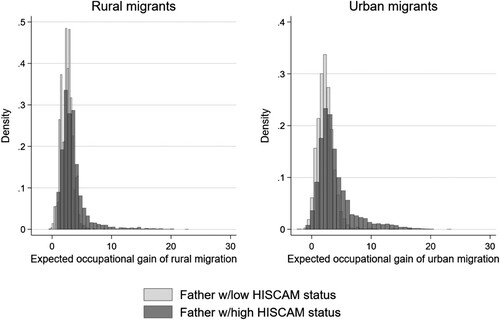
The main focus in our analysis is on the role of expected occupational gains of migration, $y_{1i}^{\ast }-y_{0i}^{\ast }$, in sons’ migration decisions. Other variables that affect the migration decision (the components of Z in equations (1) and (2)) also include both individual- and municipality-specific elements. Based on human capital theory and empirical evidence, we anticipate that a son's expectations of his occupational outcomes in rural and urban labour markets influence his mobility decision. The expected occupational gains of migrating are measured on the HISCAM scale. It is important to note that labour market opportunities, i.e. the variables in the occupational status equation, are also allowed to affect the individual's migration decision, but only through their effect on the expected occupational gains of migration, $y_{1i}^{\ast }-y_{0i}^{\ast }$. Figure 3 shows the distribution of expected occupational gains for rural and urban migrants.

Figure 3. Distribution of sons’ expected occupational gains by their migration status and parental occupational status.

If the variables in the occupational status and migration decision equations were identical, the parameters would only be identified when the model's structure and normality assumptions are exactly correct. A valid exclusion restriction should be correlated with potentially endogenous migration while being uncorrelated with occupational attainment. Our study uses some reasonable exclusion restrictions used in recent literature present in Z but not in X by including a historical municipality-level variable of households’ migration experiences. It is calculated as the number of emigrants over the total number of inhabitants in the municipality in 1865. A similar approach has been used by Rozelle, Taylor, and de Brauw (1999), McKenzie and Rapoport (2010), and Taylor and Lopez-Feldman (2010), who conclude that municipality-level variables can serve as strong exclusion restrictions as they capture the influence of exogenous historical, cultural, and geographic factors. We also include an indicator concerning whether a son was living in his municipality of birth in 1865; such individuals might be expected to have closer ties to their community and be less likely to move. This variable is a proxy for a household's place attachment, as individuals from these households might be expected to be more attached to their municipality and be less likely to move. The model's parameters are identified using these exclusion restrictions, even if the model's assumptions do not hold exactly. We further include provincial dummies in the migration equation. Sample means are presented in Table A2.

6. Results

Before proceeding to the results from the estimation of the migration equation, we first briefly look at which factors determined migrant occupational status in 1900⁶ (equation (1) in the model). We estimated occupational status equations and corrected for selection bias for both rural-rural and rural-urban migrants. We used six equations for our subsamples, utilising sons from lower-status families and sons from higher-status families.

The results (second and third columns in Table 7) yield interesting insights. The sending household's occupational status in 1865 more positively influenced the subsequent occupational status of a son from a higher-status family: the higher the father's status, the higher the son's status. This implies that they experienced higher intergenerational occupational persistence. This result is similar to what is found in Modalsli (2017). The number of servants positively affected labour market outcomes for both rural-urban and rural-rural migrants, regardless of their family background. Being the oldest son did not significantly affect sons’ subsequent occupational attainment, except for sons from families with a lower occupational status. Our results do not lend weight to the resource dilution hypothesis: family size did not have a negative effect. Rather it had a positive and significant effect on the son's occupational status in 1900 for rural-urban migrants and rural-rural migrants from higher-status families. Having a father who lived in his municipality of birth negatively affected a migrant's occupational status only for sons from higher-status families.

Table 7. Maximum likelihood results: determinants of occupational status attainment and rural-urban migration.

	Occupational status attainment Dependent variable: Son’s HISCAM status 1900						Migration decision
	Rural-urban migrants			Rural-rural migrants			Rural-urban migrants			Rural-rural migrants
	(1)	(2)	(3)	(4)	(5)	(6)	(7)	(8)	(9)	(10)	(11)	(12)
Individual characteristics	Total	Lower status	Higher status	Total	Lower status	Higher status	Total	Lower status	Higher status	Total	Lower status	Higher status
	Linear regression coefficients						Probit equation: Marginal effects
Father’s HISCAM status	0.247*** (0.0242)	0.0870 (0.114)	0.248*** (0.0305)	0.408*** (0.0330)	0.200* (0.0888)	0.457*** (0.0421)
Servants	2.156*** (0.158)	3.275*** (0.468)	2.076*** (0.177)	1.251*** (0.155)	1.976* (0.784)	1.173*** (0.160)
Son’s age	0.0589* (0.0257)	0.0425 (0.0349)	0.0655* (0.0323)	0.0222 (0.0128)	0.0389* (0.0193)	0.0173 (0.0167)	-0.00493*** (0.000245)	-0.00632*** (0.000609)	-0.00233*** (0.000290)	-0.00142*** (0.000277)	-0.00209*** (0.000633)	-0.00122*** (0.000312)
Number of siblings	0.286** (0.0880)	0.319* (0.138)	0.296** (0.110)	0.0460 (0.0532)	-0.0824 (0.0784)	0.139* (0.0689)
Eldest son	-0.421 (0.349)	0.109 (0.437)	-1.103 (0.581)	-0.190 (0.246)	-0.677* (0.301)	0.237 (0.432)
Owns resources	0.666 (0.384)	1.678 (1.207)	0.486 (0.544)	-0.435 (0.265)	2.081 (1.422)	0.285 (0.346)
Owns resources × Eldest son	-0.202 (0.566)	-0.426 (2.252)	0.338 (0.734)	-0.135 (0.354)	2.346 (2.888)	-0.450 (0.494)
Expected occupational gain $\left(y_{1i}^{\ast }-y_{0i}^{\ast }\right)$							0.00307** (0.00103)	0.0169*** (0.00449)	0.00444*** (0.00109)	-0.00379* (0.00183)	0.0224** (0.00680)	0.00136 (0.00188)
Father lived in municipality of birth	-1.339*** (0.319)	-0.328 (0.429)	-1.928*** (0.524)	-1.029*** (0.193)	-0.177 (0.280)	-1.354*** (0.271)
Son lived in municipality of birth							-0.169*** (0.00724)	-0.180*** (0.0174)	-0.129*** (0.00811)	-0.124*** (0.00840)	-0.151*** (0.0211)	-0.134*** (0.00913)
Municipality (of origin) characteristics
High share of emigrants							-0.0327*** (0.00535)	-0.0368** (0.0113)	-0.0385*** (0.00623)	-0.0304*** (0.00482)	-0.0342** (0.0113)	-0.0355*** (0.00605)
Km to nearest city	0.0125 (0.00835)	0.0108 (0.0152)	0.00869 (0.0119)	0.00155 (0.00337)	-0.00650 (0.00546)	0.00314 (0.00423)	-0.00092*** (0.0000997)	-0.00202*** (0.000237)	-0.000759*** (0.000107)	0.0000985 (0.0000837)	-0.0000099 (0.000217)	0.000146 (0.0000924)
Cities within 100 km	0.0701 (0.0552)	0.0647 (0.0788)	0.0593 (0.0748)	0.0453 (0.0325)	0.00596 (0.0446)	0.0549 (0.0468)	0.000940 (0.000653)	0.00315* (0.00144)	-0.00106 (0.000882)	-0.000102 (0.000873)	0.00167 (0.00162)	0.000579 (0.00104)
Share in secondary sector	0.0673*** (0.0192)	0.00955 (0.0259)	0.0992*** (0.0268)	0.0185 (0.0162)	-0.0294 (0.0259)	0.0342 (0.0223)	0.00155*** (0.000284)	-0.00182* (0.000723)	0.000393 (0.000393)	-0.00327*** (0.000443)	-0.00261*** (0.000789)	-0.00330*** (0.000520)
Province (of origin) characteristics (capital area is the base case)
Eastern inland	2.607** (0.930)	2.206 (1.258)	2.608 (1.638)	0.811 (0.647)	0.392 (0.882)	0.770 (0.972)	-0.104*** (0.0113)	-0.175*** (0.0248)	-0.120*** (0.0162)	-0.0199 (0.0159)	-0.0525 (0.0275)	-0.00435 (0.0205)
South-east Norway	1.181* (0.490)	1.148 (0.598)	1.096 (0.901)	-1.001* (0.464)	-1.245* (0.584)	-0.908 (0.731)	-0.0783*** (0.00735)	-0.131*** (0.0154)	-0.0669*** (0.0111)	-0.0321* (0.0125)	0.0211 (0.0225)	-0.00367 (0.0159)
South-west Norway	3.720*** (0.875)	3.151** (1.209)	3.527* (1.682)	1.279* (0.568)	1.662* (0.842)	1.008 (0.788)	-0.160*** (0.00978)	-0.200*** (0.0231)	-0.165*** (0.0135)	-0.119*** (0.0149)	-0.0506 (0.0284)	-0.0677*** (0.0183)
Western Norway	3.005** (1.056)	3.484* (1.418)	2.516 (1.647)	1.633* (0.658)	1.550 (0.904)	1.664 (0.932)	-0.132*** (0.0120)	-0.142*** (0.0269)	-0.121*** (0.0161)	-0.0718*** (0.0166)	-0.0892** (0.0306)	-0.0200 (0.0205)
Central Norway	4.318*** (1.169)	3.184* (1.576)	4.837* (1.904)	1.390* (0.691)	1.168 (0.918)	1.133 (1.028)	-0.165*** (0.0129)	-0.275*** (0.0293)	-0.154*** (0.0173)	-0.0801*** (0.0170)	-0.113*** (0.0304)	-0.0426* (0.0214)
Northern Norway	2.832* (1.219)	5.838** (1.981)	2.220 (1.805)	1.361* (0.670)	2.346* (0.918)	1.430 (0.957)	-0.178*** (0.0130)	-0.213*** (0.0329)	-0.137*** (0.0169)	-0.0846*** (0.0172)	-0.104** (0.0350)	-0.0272 (0.0213)
Constant	38.33*** (1.914)	46.69*** (5.997)	37.83*** (3.633)	32.54*** (1.835)	44.44*** (4.593)	28.55*** (2.784)
ρ1	-0.16	-0.07	-0.05	-0.08	-0.12*	-0.06
Log pseudolikelihood	-121073.9	-32238.5	-877994.8	-126107.2	-34109.0	-92139.5
Wald chi2 test	1203.2	438.4	607.1	1639.9	438.1	370.1
N	35120	8927	26193	36501	9360	27141

Notes: * p < 0.05, ** p < 0.01, *** p < 0.001. Robust standard errors in parentheses are clustered at the family level. All explanatory variables are pre-migration, measured in 1865.

We now turn our focus to the factors bearing on rural-urban migration decisions (equations (3) and (4) in the model). Columns (7)–(12) in Table 7 show the results from the probit estimation. Our main interest in the paper lies in studying whether expected labour market opportunities were a motive for rural sons to move. We obtain many interesting results. The average marginal effects show that migration due to higher expected occupational gains had a significantly more positive effect on the probability of moving to urban municipalities for sons from lower-status families (see columns (8) and (9)). This indicates that rural sons from lower-status families reacted more than their counterparts from higher socioeconomic backgrounds for even small increases in urban opportunities. The marginal effects show that for sons from lower-status families, a one-unit marginal increase in the expected occupational gain increased the probability of rural-urban migration by 1.7 percentage points, almost four times more than for the sons of higher-status families. Second, higher expected occupational gains increased the probability of rural-rural migration only for lower-status sons, and a one-unit marginal increase in the expected occupational gain increased the probability of rural-urban migration by 2.2 percentage points. We can interpret the magnitudes of these effects by using some typical examples. As Norway still had vacant land, many sons of crofters could become farmers by relocating themselves. For the son of a cotter, the prospect of moving and becoming a farmer compared to staying and becoming a cotter like his father. This is roughly represented by a HISCAM status increase from 50.18 to 54.5, increasing the odds of rural-rural migration by almost ten percentage points ($\left(54.5-50.18\right)\ast 2.2=9.5$). The insignificant coefficient for sons from higher-status families simply indicates that expected occupational advancement was not a decisive factor for rural-rural migration.

Other results are in line with standard findings from the migration literature, e.g. older sons and those with high place attachments were less prone to migrate to urban areas. The municipality-level variables were also important factors in the migration decision. Living near an urban area increased the probability of rural-urban migration in most cases. A larger share of manufacturing employment in a municipality decreased the probability of rural-rural migration. Sons coming from municipalities with an above-average share of emigrants were less likely to migrate.

To better understand the migration decisions, we present some further results from our model. We will first turn to the well-known issue of self-selection based on observables (e.g. Borjas, 1987). According to Table 8, both rural-urban and rural-rural migrants from lower-status families were slightly negatively selected on observables $(S_1<0)$. On average, they thus had observable characteristics that made them perform worse (i.e. they achieved a lower occupational status) in the destination labour markets than rural stayers would have done had they chosen to move. This result of negative selection provides empirical support for the assumed negative selection of Norwegian internal migrants because of capital constraints in Abramitzky et al. (2013). Our results of negative migrant selection on observable characteristics for sons coming from low-status families are similar to Ferrie’s (1999) results from the U.S. Rather than the ‘cream of the crop’ it was ‘the bottom of the barrel’ who migrated from the Norwegian countryside. However, the direction of selection is opposite for sons from households with a higher occupational status. Interestingly, selection to migration based on observables for this group seems to be similar to the findings for Victorian Britain (Humphries & Leunig, 2009; Long, 2005), Sweden (Eriksson, 2015) and African Americans from the U.S. South (Collins & Wanamaker, 2014). These findings suggest that migrants were the ‘cream of the crop’, i.e. having observable characteristics that made their labour market prospects bright in both rural and urban areas.

Table 8. Self-selection on observables in migration.

	Rural-urban migrants			Rural-rural migrants
	Total	Lower status	Higher status	Total	Lower status	Higher status
	(1)	(2)	(3)	(4)	(5)	(6)
Selection of migrants $S_1=E\left(y_1^{\ast }|M=1\right)-E\left(y_1^{\ast }|M=0\right)={\tilde{X}}_1{\widehat{\text{β}}}_1-{\tilde{X}}_0{\widehat{\text{β}}}_1$	−0.05 (0.044)	−0.88*** (0.046)	1.51*** (0.057)	−0.41*** (0.030)	−0.70*** (0.034)	0.34*** (0.037)

Note: * $p<0.05$, **$p<0.01$, ***$p<0.001$.

Norwegian rural-urban migrants were also expected to sort themselves from the rural population on the basis of unobservable characteristics that, while not observable for the econometrician, were known to the migrants themselves. One useful feature of the switching endogenous regression model is that we can use it to study self-selection on unobservables. These characteristics may have been energy and ambition, optimism and a tendency to search for new opportunities, a propensity for risk-taking, latent abilities or skills that portended economic success regardless of migrant status. The rho coefficient ${\rho }_1$ is a correlation coefficient for the error term of the first- and second-stage equation and indicates the presence and direction of migration selection in determining occupational status outcomes. We find evidence of endogenous selection of migration and occupation outcomes for movers driven by unobserved heterogeneity only for rural migrant sons from low-status families.­­ The negative correlation coefficient of ${\rho }_1$ implies that rural-rural movers from this occupational status group were negatively selected in terms of unobservables. The unobservable characteristics of migrants were negatively correlated with occupational status in destination municipalities. Furthermore, nonzero ${\rho }_1$ also implies that the error terms are not independent across equations, and the migration selection process cannot be treated as exogenous (Maddala, 1983), therefore additionally confirming that our choice of a model that corrects for sample selection bias was appropriate.

7. Discussion

This paper has studied internal migration from rural areas in nineteenth-century Norway. Who went where? Who stayed? Even more importantly, why did they choose to stay or move? Specifically, we have tried to answer whether Norwegian rural sons migrated to cities and towns and rural municipalities in the second half of the nineteenth century to take advantage of occupational advancement opportunities. To properly analyse their migration decisions and occupational outcomes, taking into account the effects of self-selection, we employed an endogenous switching regression model. Our main finding is that the effect of expected occupational gains on the probability of rural-urban migration differs according to the rural sons’ destination and their family background. Opportunities for occupational advancement motivated the sons from low socioeconomic backgrounds to migrate both to rural and urban municipalities; this effect was larger than for their peers from higher socioeconomic backgrounds. This implies that the probability of migration for sons from lower classes increased more when the expected labour market opportunities of staying in their rural home municipality (‘inside option’) worsened or their expected opportunities in rural or urban destinations (‘outside options’) improved. Thus, this result partly explains why people from lower classes moved to urban areas more frequently than those from higher status backgrounds (shown in Figure 1).

As mentioned, expected occupational gains were a positive and significant factor for rural-rural migrations for sons from lower classes, such as cotters’ sons. This underlines that Norwegian youth had rural opportunities when making migration choices. Unlike Great Britain and most of Western Europe that had no unsettled frontier land, Norway still enjoyed a fair amount of free soil, especially in the north. Although land in many cases was sparse, it was possible for the landless to buy land, migrate and clear a self-sustaining smallholding (Semmingsen, 1977). In addition to becoming self-owners, there was often extra income from fisheries, thus allowing them to take a step up the social ladder. Interestingly, the inside option's attractiveness may be affected by the outside option that is not explicitly included in the analysis: emigration. We have found that a high share of emigrants from a municipality is negatively associated with the probability of internal migration. A plausible explanation is that better access to land improved the attractiveness of staying in these municipalities.

We also find that expected occupational advancement did not affect the probability of rural-rural migration for sons from higher-status families as opposed to lower-status families. Since sons from higher-status families did migrate to rural areas (see Figure 1), this implies that other motives must have been important. One plausible possibility is that farmers’ sons migrated to rural municipalities because they could continue as farmers in the new location rather than end up as urban migrants (see Table 5). This emigration motive was the same motive that many farmers’ sons had when they left for the New World (Østrem, 2014).

We also find that rural migrants from lower social classes were negatively selected on observed characteristics, while the selection was positive for sons from higher socioeconomic backgrounds. Observations from contemporary historians also seem to support our finding of the negative selection of rural-urban migrants from lower classes. Eilert Sundt described how Christiania [Oslo] was in the middle of a circle of rural areas with many poor people and overwhelmed by their distress (Sundt, 1870, p. 114). Sundt also observed that a large share (36 per cent) of rural short-distance migrants to Christiania from neighbouring municipalities had received public poverty support in their municipality of origin before migrating (Sundt, 1870).

The positive selection of migrants from higher socioeconomic backgrounds, both regarding rural-rural and rural-urban migration, could be explained by the fact that many of the inputs to industrialisation were abundant in rural areas, and many Norwegian entrepreneurs built their companies on rural natural resources and were dependent on the local rural labour force. Together with fishing, these rural industrial opportunities made it possible for subsistence farmers in many places to combine farming with working in another sector without relocating. The urban opportunities open for poor self-subsistent farmers (with low and often insecure income) could, in many cases, not compete with rural opportunities from subsistence farming and seasonal income (Brox, 2000).

Our results show that the existence of rural opportunities affected rural occupational prospects and had a potentially important impact on individual migration decisions. At the height of industrialisation, a majority of Norwegian farms were small and often self-subsistent. These small self-subsistent farmers formed a large decentralised labour market reserve that did not need year-round work, creating possibilities for entrepreneurs who wanted to extract accessible rural natural resources. According to the standard economic theory, this possibility of combining income from both agricultural and industrial work also affected wages in industries located in urban areas. To recruit labour from rural areas, employers in cities and towns had to increase their wage offers, thus reducing income differences between rural and urban regions. Norway today is one of the most egalitarian countries in the world. Maybe the foundations for this were established through the way the society structured itself in the second half of the nineteenth century?

Acknowledgements

The authors wish to acknowledge the statistical offices that provided the underlying data making this research possible: The Digital Archive (The National Archive), Norwegian Historical Data Centre (University of Tromsø) and the Minnesota Population Center. National Samples of the 1865 and 1900 Censuses of Norway, Version 2.0. Tromsø, Norway: University of Tromsø, 2008.

Disclosure statement

No potential conflict of interest was reported by the author(s).

Notes

1 More detailed information about the linking procedures can be found at: https://www.nappdata.org/napp/linked_samples.shtml.

2 The number of fishermen in the 1865 census is known to be vastly understated (Thorvaldsen, 2002). There were many small-scale farmers, farmhands and cottagers who had several sources of income. Whether a freeholder or cottager was categorised as a fisherman or farmer depended on the number of farm animals he had, as well as on the importance of fishing in the area he lived in. As late as in the 1855 census, the authorities who designed the censuses did not include fisher as occupation. Their argument was that fishermen often did other work, under which they have to be categorised. Fishers often used to be farmers too and were categorised as people who sustain themselves through farming (Lie, 2002).

3 For better readability, we use an occupational class scheme based on HISCLASS here. HISCLASS (Van Leeuwen & Maas, 2011) is an international historical class scheme, created for the purpose of making comparisons across different periods, countries and languages. We use here a version of HISCLASS condensed into eight classes: Non-manual workers; Foremen and skilled workers; Fishermen; Farmers; Tenant farmers; Lower-skilled workers; Cotters; and Unskilled workers.

4 Specifically, we apply the ‘movestay’ command in Stata 16, see Lokshin and Sajaia, 2004.

5 We observe the household cross-sectionally only at one point in time. The ‘big brother’ and number of siblings indicator can thus have measurement errors, as some of the older children may already have left their home.

6 To save space, only estimates of the coefficients for migrants are reported in Table 7.

Appendix

Table A1. Summary statistics of 1865 characteristics in the final matched sample and population.

	Final matched sample Mean/SD	Population Mean/SD	Difference
Father's HISCAM status	53.68 (4.51)	53.29 (3.09)	0.39 (0.023)
Number of servants	0.53 (1.10)	0.50 (1.08)	0.03 (0.006)
Father's age	48.06 (8.47)	47.46 (8.41)	0.60 (0.045)
Number of siblings	3.23 (1.86)	3.27 (1.91)	−0.04 (0.010)
Father in the municipality of birth	0.74 (0.44)	0.703 (0.46)	0.037 (0.002)
Son's age	12.32 (7.62)	10.97 (7.58)	1.35 (0.041)
Eldest son	0.50 (0.50)	0.47 (0.499)	0.03 (0.003)
Son in the municipality of birth	0.94 (0.23)	0.86 (0.342)	0.08 (0.001)

Notes. Table includes sons of age 0–35 in 1865 who had 35–70 year old rural fathers with an occupation (matched = 42,219; population = 210,340).

Table A2. Sample means and standard deviations for rural-urban migrants, rural-rural migrants and rural stayers.

	Rural-urban migrants						Rural-rural migrants						Rural stayers
	Total		Lower levels of wealth		Higher levels of wealth		Total		Lower levels of wealth		Higher levels of wealth		Total		Lower levels of wealth		Higher levels of wealth
	Mean	S.d.	Mean	S.d.	Mean	S.d.	Mean	S.d.	Mean	S.d.	Mean	S.d.	Mean	S.d.	Mean	S.d.	Mean	S.d.
Household and individual characteristics Son's HISCAM status in 1900	57.6	10.64	55.0	8.88	59.3	11.30	54.8	7.80	53.1	6.67	55.8	8.24	54.4	4.89	53.0	5.00	54.8	4.78
Father's HISCAM status	54.2	7.85	49.2	1.85	57.3	8.53	53.4	5.61	49.5	1.60	55.8	5.82	53.6	3.23	49.6	1.46	54.9	2.54
Number of servants	0.6	1.33	0.1	0.49	0.9	1.57	0.4	1.12	0.1	0.32	0.6	1.34	0.5	1.05	0.1	0.36	0.7	1.15
Son's age	10.9	6.75	10.2	6.26	11.3	7.01	11.5	7.08	11.3	6.70	11.7	7.29	12.8	7.90	11.8	7.44	13.1	8.01
Eldest son	44%	0.50	48%	0.50	42%	0.49	47%	0.50	53%	0.50	44%	0.50	52%	0.50	54%	0.50	51%	0.50
Number of siblings	3.4	1.82	3.1	1.62	3.6	1.90	3.2	1.84	2.9	1.65	3.5	1.91	3.2	1.87	2.8	1.66	3.3	1.91
Father owns land or business	37%	0.48	3%	0.18	58%	0.49	42%	0.49	2%	0.14	65%	0.48	58%	0.49	2%	0.14	75%	0.43
Father in the municipality of birth	59%	0.49	60%	0.49	59%	0.49	65%	0.48	63%	0.48	66%	0.47	78%	0.41	72%	0.45	80%	0.40
Son in the municipality of birth	86%	0.35	87%	0.33	85%	0.36	89%	0.31	92%	0.28	88%	0.32	97%	0.18	96%	0.19	97%	0.18
Expected gain of migrating	3.4	2.74	2.4	1.51	4.0	3.13	3.3	2.36	2.5	1.75	3.7	2.71	3.5	2.18	2.6	1.28	3.8	2.39
Municipality (of origin) characteristics
High share of emigrants	17%	0.37	19%	0.39	15%	0.36	20%	0.40	0.3	0.44	18%	0.38	23%	0.42	31%	0.46	21%	0.41
Share in secondary sector	13%	9.83	14%	9.51	12.9	10.02	9.6	8.17	11%	8.10	9%	8.13	8%	7.75	10%	8.02	7.9	7.60
Nearest city (km)	26.3	28.13	24.1	22.25	27.6	31.17	42.6	38.96	36.8	33.63	46.0	41.38	47.2	41.90	41.5	37.30	48.9	43.03
Nearby urban municipalities (within 100 km)	12.9	9.03	13.4	8.70	12.6	9.21	9.2	8.89	10.2	8.72	8.6	8.94	7.1	8.05	8.1	8.21	6.8	7.98
Province (of origin) characteristics
Capital area	15%	0.37	20%	0.40	14%	0.34	7%	0.26	9%	0.30	6%	0.23	5%	0.20	7%	0.25	4%	0.19
Eastern inland	10%	0.30	15%	0.36	7%	0.26	13%	0.33	20%	0.40	9%	0.28	11%	0.31	20%	0.40	8%	0.27
South-East Norway	36%	0.48	36%	0.48	36%	0.48	27%	0.44	30%	0.46	25%	0.43	18%	0.39	21%	0.41	17%	0.38
South-West Norway	13%	0.33	9%	0.29	15%	0.35	12%	0.33	9%	0.29	14%	0.35	15%	0.36	10%	0.30	17%	0.38
Western Norway	14%	0.35	12%	0.32	15%	0.36	17%	0.38	13%	0.33	19%	0.40	20%	0.40	15%	0.36	22%	0.41
Central Norway	6%	0.23	6%	0.25	5%	0.22	8%	0.28	11%	0.31	7%	0.25	10%	0.30	16%	0.37	9%	0.28
Northern Norway	6%	0.23	2%	0.15	8%	0.27	16%	0.36	8%	0.26	20%	0.40	21%	0.40	11%	0.31	24%	0.43
N	5355		2061		3294		6790		2498		4292		30074		6906		23168

References

- Abramitzky, R., Boustan, L. P., & Eriksson, K. (2012). Europe's tired, poor, huddled Masses: Self-selection and Economic outcomes in the Age of Mass migration. The American Economic Review, 102, 1832–1856.
- Abramitzky, R., Boustan, L. P., & Eriksson, K. (2013). Have the poor always been less likely to migrate? Evidence from inheritance practices during the age of mass migration. Journal of Development Economics, 102, 2–14.
- Becker, G. S., & Tomes, N. (1986). Human capital and the rise and fall of families. Journal of Labor Economics, 4, 1–39.
- Bhashkar, M., & Miguel, A. (2015). Using occupation to measure intergenerational mobility. The Annals of the American Academy of Political and Social Science, 657, 174–193.
- Black, S. E., Devereux, P. J., & Salvanes, K. G. (2005). The more the merrier? The effect of family size and birth order on children's education. The Quarterly Journal of Economics, 120, 669–700.
- Blake, J. (1981). Family size and the quality of children. Demography, 18, 421–442.
- Borjas, G. (1987). Self-Selection and the earnings of immigrants. The American Economic Review, 77, 531–553.
- Brox, O. (2000). Bygd og by i det norske klassesamfunnets historie [Village and city in the history of the Norwegian class society]. Vardøger, 26, 126–135.
- Brox, O. (2013). Fattigdom og framgang: Alternative fortider? - Norsk industrialisering i komparativt lys [Poverty and prosperity: Alternative pasts? - Norwegian industrialization in a comparative light]. Norsk antropologisk tidsskrift, 24, 169–180.
- Bull, E. (1966). Håndverkssvenner og arbeiderklasse i kristiania - sosialhistoriske problemer [craftsmen and working class in kristiania - social historical problems]. Historisk Tidsskrift, 45, 89–113.
- Collins, W. J., & Wanamaker, M. H. (2014). Selection and Economic gains in the Great migration of African Americans: New Evidence from linked census data. American Economic Journal. Applied Economics, 6, 220–252.
- Eriksson, B. (2015). Dynamic Decades: A micro perspective on late nineteenth century Sweden Vol. PhD thesis. Department of Economic History. Lund University.
- Ferrie, J. P. (1996). A New sample of males linked from the Public Use Microdata sample of the 1850 U.S. Federal Census of population to the 1860 U.S. Federal Census manuscript schedules. Historical Methods: A Journal of Quantitative and Interdisciplinary History, 29, 141–156.
- Ferrie, J. P. (1999). How ya gonna keep ‘em down on the farm [when they’ve seen Schenechtady]? Rural to urban migration in nineteenth-century America 1850–1870. Working paper. Northwestern University. Department of Economics.
- Gjerdåker, B. (1981). Vesser i Nordlanda 1800-1865. In Gjerdåker, B. (red), På flyttefot: Innanlands vandring på 1800-talet [On the move: Domestic migration in 19th century] (pp. 36-60). Oslo: Samlaget.
- Goeken, R., Huynh, L., Lynch, T. A., & Vick, R. (2011). New Methods of Census Record linking. Historical Methods: A Journal of Quantitative and Interdisciplinary History, 44, 7–14.
- Heckman, J. (1974). Shadow prices, market wages, and Labor supply. Econometrica, 42, 679–694.
- Heckman, J. (1976). The Common Structure of Statistical Models of Truncation, Sample Selection and Limited Dependent Variables and a Simple Estimator for Such Models. Annals of Economic Social Measurement, 5, 475–492.
- Heckman, J. (1979). Sample Selection Bias as a Specification Error. Econometrica, 47, 153–161.
- Helle, K. (2006). Norsk byhistorie: Urbanisering gjennom 1300 år [Norwegian history of towns: Urbanisation through 1300 years]. Oslo: Pax.
- Humphries, J., & Leunig, T. (2009). Was dick whittington taller than those he left behind? Anthropometric measures, migration and the quality of life in early nineteenth century London? Explorations in Economic History, 46, 120–131.
- Knigge, A., Maas, I., Van Leeuwen, M. H. D., & Mandemakers, K. (2014). Status attainment of siblings during modernization. American Sociological Review, 24, 547–560.
- Lambert, P. S., Zijdeman, R. L., Van Leeuwen, M. H. D., Maas, I., & Prandy, K. (2013). The construction of HISCAM: A stratification scale based on social interactions for Historical comparative research. Historical Methods: A Journal of Quantitative and Interdisciplinary History, 46, 77–89.
- Lie, E. (2002). Socio-economic categories in Norwegian censuses up to about 1960. In J. Carling (Ed.), Nordic demography: Trends and differentials (pp. 31-51). Oslo: Unipub forlag.
- Lokshin, M., & Sajaia, Z. (2004). Maximum likelihood estimation of endogenous switching regression models. The Stata Journal, 4, 282–289.
- Long, J. (2005). Rural-Urban migration and socioeconomic mobility in Victorian britain. Journal of Economic History, 65, 1–35.
- Long, J. (2013). The surprising social mobility of Victorian britain. European Review of Economic History, 17, 1–23.
- Long, J., & Ferrie, J. (2013). Intergenerational occupational mobility in Great Britain and the United States Since 1850. The American Economic Review, 103, 1109–1137.
- Maddala, G. S. (1983). Limited-dependent and qualitative variables in econometrics. Cambridge: Cambridge University Press.
- McKenzie, D., & Rapoport, H. (2010). Self-selection patterns in Mexico-U.S. Migration: The role of migration networks. Review of Economics and Statistics, 92, 811–821.
- Minnesota Population Center. (2020). Integrated Public Use Microdata Series, International: Version 7.3 [dataset]. Minneapolis, MN: IPUMS.
- Modalsli, J. (2017). Intergenerational mobility in Norway, 1865–2011. The Scandinavian Journal of Economics, 119, 34–71.
- Myhre, J. E. (1977). Urbaniseringen i Norge i industrialiseringens første fase ca.1850–1914 [urbanization in Norway in the first phase of industrialization ca.1850–1914]. In G. A. Blom (Ed.), Urbaniseringsprosessen i Norden : det XVII. nordiske historikermøte, Trondheim 1977: Industrialiseringens første fase [The urbanization process in the Nordic countries: XVII Nordic historians’ meeting, Trondheim 1977: The first phase of industrialization], Vol. 3 (pp. 9–90). Oslo: Universitetsforlaget.
- Myhre, J. E. (1981). Det livligste “vexel-forhold” [The most lively “interrelation”]. In B. Gjerdåker (Ed.), På flyttefot: Innanlands vandring på 1800-talet [On the move: Domestic migration in 19th century] (pp. 125–145). Oslo: Samlaget.
- Nakosteen, R., & Zimmer, M. (1980). Migration and income: The question of self-selection. Southern Economic Journal, 46, 840.
- Østrem, N. O. (2014). Norsk utvandringshistorie [Norwegian emigration history]. Oslo: Samlaget.
- Roy, A. (1951). Some thoughts on the distribution of earnings. Oxford Economic Papers, 3, 135–146.
- Rozelle, S., Taylor, J. E., & de Brauw, A. (1999). Migration, remittances, and agricultural productivity in China. American Economic Review, 89, 287–291.
- Ruggles, S., Fitch, C. A., & Roberts, E. (2018). Historical census record linkage. Annual Review of Sociology, 44, 19–37.
- Ruggles, S., Roberts, E., Sarkar, S., & Sobek, M. (2011). The North Atlantic Population project: Progress and prospects. Historical Methods: A Journal of Quantitative and Interdisciplinary History, 44, 1–6.
- Semmingsen, I. (1977). Origin of Nordic emigration. American Studies in Scandinavia, 9, 9–16.
- Sjaastad, L. A. (1962). The costs and returns of human migration. Journal of Political Economy, 70, 80–93.
- Statistisk Sentralbyrå. (1969). Historisk Statistikk 1968. In Norges Offisielle Statistikk XII Vol. 245.
- Stewart, J. I. (2006). Migration to the agricultural frontier and wealth accumulation, 1860–1870. Explorations in Economic History, 43, 547–577.
- Stewart, J. I. (2012). Migration to U.S. Frontier cities and job opportunity, 1860–1880. Explorations in Economic History, 49, 528–542.
- Sundt, E. (1870). Om fattigforholdene i Christiania [about the poverty situation in Christiania]. Christiania: J. Chr. Gundersens boktrykkeri.
- Taylor, J. E., & Lopez-Feldman, A. (2010). Does migration make rural households more productive? Evidence from Mexico. Journal of Development Studies, 46, 68–90.
- Thorvaldsen, G. (2002). The Norwegian Historical Data centre. In P. K. Hall, R. McCaa, & G. Thorvaldsen (Eds.), Handbook of International Historical Microdata for population research (pp. 179-206). Minnesota Population Center.
- Thorvaldsen, G. (2011). Using NAPP census data to construct the Historical population register for Norway. Historical Methods: A Journal of Quantitative and Interdisciplinary History, 44, 37–47.
- Tobin, J. (1958). Estimation of relationships for limited dependent variables. Econometrica: Journal of the Econometric Society, 24–36.
- Van Leeuwen, M. H. (2009). Social inequality and mobility in history: introduction. Continuity and change, 24, 399–419.
- Van Leeuwen, M. H. D., & Maas, I. (2011). Hisclass: A historical international social class scheme. Leuven: Leuven University Press.
- Van Leeuwen, M. H. D., Maas, I., & Miles, A. (2004). Creating a Historical International standard classification of occupations An exercise in multinational Interdisciplinary cooperation. Historical Methods: A Journal of Quantitative and Interdisciplinary History, 37, 186–197.
- Yezer, A. M, & Thurston, L. (1976). Migration patterns and income change: implications for the human capital approach to migration. Southern Economic Journal, 693–702.