Lithuanian economy, 1919–1940: stagnant but resilient. The first inter-war GDP time-series estimates and their implications

ABSTRACT

This paper presents the first attempt to estimate the GDP time series for inter-war Lithuania, tracking the country's annual performance from 1919 until its incorporation into the USSR in 1940, and situating Lithuania within the wider East-Central European economic landscape. The research provides robust evidence that, contrary to prior beliefs, Lithuania was a stagnant economy, resembling other newly established agricultural states such as Estonia and Poland in terms of its GDP growth rate. By 1940, Lithuania remained on the economic periphery of Europe, yet it demonstrated significant resilience during the Great Depression, with no contraction in its GDP per capita between 1929 and 1938. This paper helps fill one of the remaining gaps in Europe's historical national accounts, making it an essential resource for analysing the divergent growth patterns in East-Central Europe.

SANTRAUKA

Straipsnyje pateikiami pirmieji Lietuvos BVP laiko eilutės duomenys visiems tarpukario nepriklausomybės metams. Rezultatai atskleidžia, jog Lietuvos ekonomika iki sovietinės okupacijos augo lėtai, panašiu į kitų jaunų agrarinių valstybių, kaip Lenkija ar Estija, tempu. Nors tarpukario Lietuva priklausė Europos ekonominiam paribiui, ji sėkmingai atlaikė Didžiosios depresijos krizę. Tai rodo šalies atsparumą tarptautiniams sukrėtimams. Straipsnyje pateikiami tarpukario Lietuvos duomenų rinkiniai yra ir pagrindas tolesnei diskusijai apie ilgalaikius Baltijos šalių ir Centrinės Europos ekonominius skirtumus.

KEYWORDS:

• Lithuanian GDP
• inter-war
• Baltic states
• Eastern Europe

JEL CODES:

• N14
• O47

1. Introduction

The aim of this paper is to provide the first estimation of the GDP time-series for inter-war Lithuania, shedding light on the country's overall and sectoral performance from the start of its sovereign governance in 1919 until its annexation by the USSR in 1940. Lithuania is one of the three neighbouring Baltic States (alongside Latvia and Estonia) which have been hitherto excluded from nearly all economic history studies, such as Aldcroft and Morewood (1995), Berend (2006), and Broadberry and O'Rourke (2010) due to a lack of reliable historical national accounts (HNA) statistics. This paper is an attempt to fill this gap. Moreover, it seeks to position inter-war Lithuania in a broader East-Central European economic context, laying the groundwork for explaining the origins of the region's divergent growth patterns.

The availability of GDP data in Lithuania, Latvia, and Estonia lags behind other economies in the Baltic Sea region. In contrast, Swedish historical national accounts have been regularly updated and are considered among the most robust worldwide (Edvinsson, 2013b; Krantz, 1988). In more recent years, O. Grytten has extended and updated the Norwegian GDP series using the double deflation technique for the production side accounts, and also provided estimates from the expenditure side (Grytten, 2021). Of particular relevance to this study are the comprehensive GDP estimates for Finland, a country that emerged after World War I together with Lithuania, and has some of the best series by production, income, and expenditure approach among European countries, thanks to the works of R. Hjerppe and the favourable data situation there (Hjerppe, 1989). While this study draws on these works, limited Lithuanian sources and literature allow for a robust yet imperfect first attempt at a single-side estimation currently.

Recent years have brought some progress to the HNA of the Baltics. In 2003, Estonia published its first and, so far, only GDP per capita time series for 1923–1938 (Valge, 2003). Although lacking in depth, these production-side estimates still offer a preliminary insight into the inter-war Estonian economy. In Lithuania a detailed output-side estimate of 1937 GDP was produced in 2019 (Klimantas & Zirgulis, 2020), followed in 2020 by indirect income-side estimations for 1913, 1922, 1929 and 1938 (Norkus & Markevičiūtė, 2021) covering all three Baltic states.¹ Similarly to the Lithuanian 1937 estimate, a comprehensive output-side study of Latvia's 1935 GDP was published in 2022 (Norkus et al., 2022). Finally, a paper aimed at providing the time-series of Latvian 1920–1939 GDP has come out in parallel to the present study (Klimantas et al., 2023, august). There have been previous attempts to estimate historical aggregate production in the Baltics, all of which have been thoroughly reviewed in Norkus and Markevičiūtė (2021). These efforts, however, suffer from serious methodological and data issues, being incomparable to the results of this paper.

No previous attempts have been made to estimate the time-series of GDP for inter-war Lithuania. During the Cold War, Soviet economists largely neglected the capitalist Lithuanian economy, resulting in the lack of production of either NMP or single sector series. Additionally, the inter-war Lithuanian statistical office was weak (Norkus et al., 2019, p. 37), with its archive having been destroyed in 1944 (Dagys, 1959, may, p. 140). As a result, scholars since 1990 have had extremely limited literature to work with. In comparison, Edvinsson (2013a, p. 42) cites seven different studies on the 17th and 18th century Swedish long-run agricultural trends which he was able to utilise in his research. Similarly, the Finnish and Norwegian GDP studies made extensive use of individual sector analyses by other authors Hjerppe (1989, p. 26) and Grytten (2021, p. 187). Since 1990, almost no literature has been produced on inter-war Lithuanian economic trends, making Norkus and Markevičiūtė's 2021 study the only comprehensive one to date. They were able to make indirect income-side estimates after discovering scattered proxy wage data, insufficient for proper compilation of income-side accounts. With demand-side sources being even more scarce,² this paper attempts to construct the GDP series employing a combination of both production-side and income-side data. Such procedure is standard in HNA even for later periods in advanced countries (e.g. Swedish industrial series were constructed in this way for periods before 1931, see Schön, 1988, p. 90).

First, the paper compiles a database of constant-price value-added indices for 21 sectors from scratch. It then uses the 1937 weights from the Klimantas & Zirgulis benchmark GDP and other sources to arrive at a constant-price 1919–1940 GDP series. Being aware of the issues of changing relative prices, this paper assumes no major structural shifts during the 22 years in question and follows the approach of Crafts and Harley (1992, p. 707) to obtain value-added figures for the years before and after 1937. Finally, it converts the results into GK$₁₉₉₀, using a PPP conversion ratio from the same benchmark study, producing internationally comparable GDP per capita time-series.³

The findings of this study indicate that Lithuania was a typical agricultural state on the European periphery when it emerged independent in 1918–1919 and remained so throughout the inter-war period. While the country's per capita income was somewhat lower than regional averages, it was able to weather the Great Depression better than many other states. These findings are important in the context of debates about crisis theory and shed light on pre-Soviet growth in capitalist Europe. Furthermore, this study lays the groundwork for future improvements, expansions, and reproductions of time-series data for the remaining Baltic states.

The paper is structured as follows: Section 2 begins with an explanation of the methodology used in this study and an overview of the benchmark GDP figures. Subsection 2.1 describes the territorial, population, and price fluctuations that occurred in inter-war Lithuania. Subsections 2.2, 2.3 and 2.4 present the value-added estimation procedures for the major sectors, the final GDP figures and their limitations respectively. Section 3 discusses the results obtained, while Section 4 concludes the study. Estimation procedures and sources are further detailed in the Appendices.

2. Estimating Lithuanian GDP

There are three alternative ways of estimating a country's gross domestic product: supply side (by aggregating value-added created in all economic sectors), demand side (by adding up expenditures of all subjects in the economy) and income side (by aggregating incomes of all subjects in the economy).

As the data is insufficient for applying any of these three direct methods for the entire inter-war period, this paper follows the sector of origin benchmark-extrapolation approach. At least one detailed supply side benchmark GDP estimate is required for employing this method. The work of Klimantas and Zirgulis (2020) (with a slight correction from Norkus et al. (2022) and improvements provided in Appendix 1) serves this purpose well as it provides sophisticated estimates of 1937 value-added created in all economic sectors distinguished by the UN's System of National Accounts and aggregates them into a GDP at market prices figure (see Table 1). To obtain GDP series for more than one year, constant-price movement of each economic sector has to be estimated using correlated data. In this way, corresponding sectoral volume indices are compiled. These indices are then aggregated into an index of total gross value-added (GVA) at basic prices using the weights from the benchmark figure. The process is summarised by the following formula: $indexGD{P}_t=\sum _{i=1}^n{W}_{i|benchmarkyear}\times indexSecto{r}_{it},$where indexGDP_t is the GDP index value in year t, W_i is the % weight of the ith sector in total GDP at the benchmark year and indexSector_it is the value-added index figure of the ith sector in year t. Once indexGDP_t is obtained, it can then be multiplied by the actual GDP value in the benchmark year to arrive at complete series (see Table 1).

Table 1. Lithuanian benchmark GDP by main sectors of origin in 1937 at current prices.

	Value-added, million LTL	Weight in total
Agriculture, forestry & fishing	823.0	44.1%
Industry	279.7	15.0%
Construction	68.2	3.7%
Trade. accommodation & food service activities	335.6	18.0%
Transportation & communications	51.9	2.8%
Financial, insurance & real estate activities	115.4	6.2%
Public & social security administration, defence, education & health	142.4	7.6%
Other services	51.1	2.7%
Total gross value-added at basic prices	1867.2	100.0%
Taxes less subsidies on products	68.3
GDP at market prices	1935.5

Source: Klimantas and Zirgulis (2020, pp. 239–241), with revisions described in Appendix 1.

In this paper, the economy is divided into 22 sectors for which constant price value-added indices are compiled (Section 2.2). These indices are aggregated into GDP and GDP per capita at constant prices series in Section 2.3. A PPP conversion ratio from Klimantas & Zirgulis is used in the same section to arrive at internationally comparable estimates.

The sector of origin approach remains a standard procedure in HNA (see Broadberry et al., 2015; Pryor et al., 1971; van Zanden & van Leeuwen, 2012). While there has been some debate on the reliability of single-year benchmarks, the controversy has gradually lost its ground (see Broadberry & Burhop, 2007, 2008, 2010). To check the reliability of estimates, the results obtained in this paper are measured against the latest income-side GDP estimates for 1922, 1929 and 1938 from Norkus and Markevičiūtė (2021, p. 603) at the end of the estimation section.

2.1. Territory, population and prices

Lithuania declared independence on February 16th, 1918 while under German occupation. Its government, however, took control only after Germany lost the war in late 1918 (that is why virtually no data exists for 1918). Independence wars which took place in 1919–1920 resulted in a firm establishment of Lithuanian statehood at the cost of capital Vilnius region which was lost to Poland (Figure 1).

Figure 1. Map of Lithuania, 1918–1940. Own work, based on Gaučas et al. (2001), Vaskela (2014, pp. 88–89), and calculations in this paper.

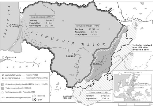
Lithuania received a tiny Baltic coastal strip after the 1921 border exchange with Latvia and gained full access to the sea in early 1923 following the annexation of autonomous Klaipėda region.⁴ For the most of inter-war Lithuania's existence, statistical sources refer to the territory without Klaipėda region (1921–1922 borders) or with Klaipėda region (1923–1938 borders). Fortunately, for the purposes of this paper, constant territory without Klaipėda region holds even when sources refer to 1919 when the Lithuanian territory was highly unstable. The last territorial changes happened in 1939 with Germany annexing Klaipėda region in March and the Soviet Union returning a part of the Vilnius region (referred to as Vilnius area later in the text) to Lithuania in October. Finally, on June 15th, 1940 the country was invaded and annexed by the USSR. However, economic incorporation of Lithuania into the Soviet system was only completed in 1941 (Visuotinė Lietuvių Enciklopedija, 2020) and thus this paper includes the year 1940 into the estimates as well. The series compiled in this paper refer to the actual territory of Lithuania in the respective year. All three major territorial changes happened either at the beginning of a year or at one's end. Thus, most statistical data for 1919–1922 and 1939 cover the area without Klaipėda and Vilnius regions, 1923–1938 with Klaipėda region but without Vilnius region and 1940 with Vilnius region but without Klaipėda region. Only slight adjustments were needed to estimate the average yearly population.

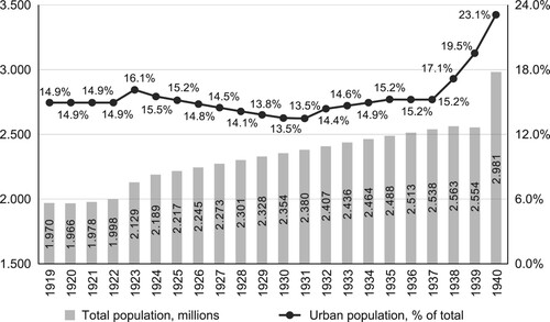
Regarding both territorial and corresponding population changes, all figures provided in this paper refer to the actual territory and the average population of the respective year unless stated otherwise (see Figure 2).

Figure 2. Mean annual population and urbanisation level in Lithuania, 1919–1940. Calculated by the author based on the end-of-the-year population figures, adjusted for dates of territorial changes to arrive at annual mean figures. Urban/rural figures are extrapolated for 1919–1922 and interpolated for 1924–1929 and 1933–1934. Sources: sections on population in Lietuvos statistikos metraštis (Centralinis Statistikos Biuras, 1927, 1929b, 1939a, 1940a; Meškauskas, 1994, p. 252; Visuotinė Lietuvių Enciklopedija, 2016).

The deflation of the 1930s (see Table 2) will be an important piece of this paper when dealing with sectors for which only monetary data exists. Until October 1922 Lithuania used the Ostmark, a German currency tied to the inflationary Mark. Once it began transmitting hyperinflation to Lithuania, it was replaced by the Lithuanian Litas (LTL) which circulated until 1941.

Table 2. Price indices in inter-war Lithuania, 1937 = 100.

Year	Minimum cost of living	General price index	Construction price index	Ostmark/LTL exchange rate
1919	[252]	[304]	[298]	2:1
1920	[755]	[912]	[893]	6:1
1921	[1259]	[1520]	[1488]	10:1
1922 I–X	[5035]	[6080]	[5952]	40:1
1922 X–XII	126	152	149
1923	156	188	184
1924	185	211	207
1925	201	227	201
1926	190	208	189
1927	189	209	179
1928	183	209	174
1929	179	201	170
1930	160	168	165
1931	149	146	154
1932	126	119	132
1933	109	100	107
1934	102	95	99
1935	91	82	88
1936	91	86	83
1937	100	100	100
1938	102	100	106
1939	107	105	111
1940	137	140	140

Note: Figures in brackets refer to the period of Ostmark circulation, figures in italic are extrapolated from the general price index. Sources: Centralinis Statistikos Biuras (1924a, p. 13), Centralinis Statistikos Biuras (1924b, p. 16), Centralinis Statistikos Biuras (1924c, p. 8), Centralinis Statistikos Biuras (1924d, p. 9), Centralinis Statistikos Biuras (1924e, p. 10), Centralinis Statistikos Biuras (1924f, p. 10), Centralinis Statistikos Biuras (1924g, p. 10), Centralinis Statistikos Biuras (1924h, p. 10), Centralinis Statistikos Biuras (1924i, p. 10), Centralinis Statistikos Biuras (1924j, p. 10), Centralinis Statistikos Biuras (1940f, pp. 159–160), and Vaskela (2011a, 2011b).

2.2. Value-added indices

This section provides a broad overview of the index calculations of the main sectors of origin. Full VA series, sources and individual cross-checks are provided in Appendix 2. Small subsectors are combined into larger ones using volume weights from Klimantas and Zirgulis (2020) unless stated otherwise.

The central assumption used in this paper is the one of unchanging constant-price 1937 value-added-to-output ratio (single deflation). Double deflation – when both output and intermediate consumption (IC) values have separate annual change indices – is the preferred method for more recent periods. While gaining popularity in the Nordic countries due to their exceptional historical data coverage (see Grytten, 2021, p. 194; Krantz & Schön, 2007, p. 25), double deflation is still highly uncommon in historical national accounting more broadly (Lobell et al., 2008, p. 151). In the case of inter-war Lithuania, reliable input data is limited to the late 1930s. With Lithuania's per capita income in 1937 amounting to less than half of British income in 1913 (Bolt et al., 2018), coupled with the absence of industrial censuses and only one agricultural census conducted, the economic development and statistical coverage in inter-war Lithuania lagged considerably behind pre-WWI Britain and other advanced nations. Given that single deflation is the prevailing method for periods prior to 1913 in many industrialising and advanced economies (Thomas & Feinstein, 1990, pp. 427–428, 440), the current availability of Lithuanian inter-war data precludes the possibility of employing double deflation.

Empirical findings by Lobell et al. (2008, pp. 148–153) reveal that single deflation is more likely to affect figures in the short run rather than the long run, thereby being a constraining factor in the present 22-year study. Nevertheless, the technique is also more likely to affect the individual sectors than the aggregate which tends to be counterbalanced by compensatory trends where outputs from one sector become inputs in another. According to Thomas and Feinstein (1990, p. 433) single deflation causes additional issues when the base year is chosen either early or late in the period. They argue that selecting a late benchmark year might lead to an overestimation of growth. However, since the growth rates generated in this paper are already quite modest (and even lower than those in the cross check study), it is assumed that the choice of 1937 as the base year has not artificially inflated the growth rates. Estimates of the potential impact of using single deflation on the figures obtained in this paper are presented in the limitations section.

Similarly, this paper assumes zero change in relative prices – a standard assumption in short periods without major productivity changes, particularly when the main objective is a constant rather than current-price series. (See, for example, Harley, 1982, p. 270.)

Another general assumption is related to the 1940 data. CSB issued its last statistical bulletin in October 1940 before being shut down by the Soviet authorities. An assumption applied in the paper is that full 1940 figures can be extrapolated from 1939 using the 1939-to-1940 ratio from the first 9 months.

2.2.1. Agriculture, forestry & fishing

To estimate the volume indices of VA in agriculture, this paper uses physical output figures of 10 crops and 7 animal product categories for which published and archival data was obtained. These include rye, wheat, barley, oats, peas, linseed, flax fibre, potatoes and sugar beet for crops and milk, other cattle output (meat, hides), pig, sheep, horse farming, egg production and other livestock for animal production. Weights used for aggregating these individual series into crop and output indices are taken from the 1937/1938 Agricultural accounting survey results (Žemės Ūkio Rūmai, 1940, pp. 37–39).⁵ The product categories used to aggregate the series covered 73% of crop output and up to 100% of livestock production in 1937. This displays the level of confidence in the estimates of the two most important subsectors in the Lithuanian inter-war economy.

Forestry and fishing indices are compiled from the physical amounts of forestry sold and the weight of fish caught. Drastic shifts in fishing values in 1921, 1923 and 1939 reflect territorial changes.⁶

2.2.2. Industry

Inter-war Lithuanian industrial statistics are exceptionally poor. Figures of industrial output are only available from 1929 and are highly unreliable.⁷ Locating separate output data of the most important industrial sectors such as food processing proved impossible as well. Therefore, this paper uses productivity-adjusted employment data to approximate industrial growth. To estimate the total number of workers in Lithuania, incomplete employment statistics are enhanced using industrial certificate data. The resulting dataset is then weighed by the real wages of unskilled workers to account for the productivity change. The resulting index is assumed to be representative of the constant-price movement in the industrial sector, including small industrial enterprises and crafts, covered in the 1937 benchmark study as part of the industrial sector (Klimantas & Zirgulis, 2020, p. 243). It was impossible to precisely evaluate the industrial production outside regular employment. Nevertheless, the contribution of households is included as part of undifferentiated household income covered in Table A8 in Appendix 2.

2.2.3. Construction

To account for the change in construction sector VA, this paper uses physical amounts (number of buildings or cubic space) of new objects constructed (residential & non-residential buildings and infrastructure projects) where possible. Where such data is unavailable, monetary values of the capital invested, deflated by the construction costs index from Table 2 are used. Exceptions are the years 1919–1921 and 1940 for which no data on housing construction exists and hence the index values are extrapolated from the change in rural and urban population.

2.2.4. Trade and accommodation & food service activities

The change in value-added of trade is approximated by the movement of combined VA of marketed agricultural and industrial goods (see Broadberry et al., 2015, p. 168; Pryor et al., 1971, p. 56). The reflated value of imports must be included as well. In case of agricultural goods, the proportion of marketed (sold by farmers) production is obtained from the Agricultural accounting survey results (except for forest and fishing products, all of them are assumed to have reached the market). In the case of industrial goods, it is assumed that 100% of them were marketed. The entire value of imports is assumed to have been marketed too.

Value-added of accommodation and food service activities is assumed to have moved in line with the urban population (from Figure 2) as there is no better-correlated data available.

2.2.5. Transportation & communications

Railway transportation series is obtained from the changes in passenger-km and ton-km as physical indicators. Land transportation index is obtained from the change in number passenger-km of buses (land freight was negligible and is considered to be 0).⁸ Water transportation series is estimated using the turnover of physical weight of goods transported via marine and inland waterways. Postal service activity is approximated by the respective employment figures. Changes in telephone and radio services are estimated using the movement of the number of users of the respective amenities. Finally, the telegraph series is obtained from the annual number of outbound telegrams.

2.2.6. Financial, insurance & real estate activities (FIRE)

The financial activities series is estimated from the change in the difference between interest receipts from loans and interest expenses on deposits in Lithuanian credit institutions, deflated by the cost of living index (Table 2). Insurance activity data (premiums received minus premiums paid) is only available for years between 1928 and 1939. For the rest of the inter-war period, the paper assumes that insurance activities moved together with financial activities.

The real estate index is compiled from reflated changes in the ‘taxable base’ which is obtained by dividing the annual real estate tax income by the respective tax rate. Only the urban real estate activities are considered as the rural ones are part of undifferentiated household incomes in Other services. The index is subject to further improvement as urban real estate tax was levied on all theoretical rents receivable if all the property was leased (Dargis, 1975, p. 68; Micuta, 1930/1990, p. 183). It proved impossible to identify the proportion of the housing stock which was actually rented. An unusually high share of real estate (see Table 1) in GDP arises from extreme undersupply of apartments in inter-war Lithuanian cities (Kuodys, 2012).

2.2.7. Public & social security administration, defence, education & health

Public administration, defence and education in inter-war Lithuania were non-market sectors (except for several private schools). The changes in VA of these activities are thus reliably approximated by the movement of the respective employment figures. To compile an index of public administration, this paper uses the number of state servants available for 1921–1938 (with gaps filled by interpolation). Figures for the rest of the years are extrapolated using population changes. It is assumed that social security and municipal administration (7–9% of total public administration wages paid Centralinis Statistikos Biuras, 1937a, p. 184, 189) moved together with the public administration index.

A defence index is compiled from the annual average numbers of active soldiers in the Lithuanian armed forces. Movement of the education sector is obtained from changes in the numbers of teaching staff in primary, secondary and tertiary education institutions weighed by the wage disparities between these groups. Finally, the healthcare value-added series is constructed from the change in the number of doctors in Lithuania as no consistent figures for other types of medical staff are available (private healthcare is assumed to have moved together with public).

2.2.8. Other services

Other services in this paper include (1) arts, entertainment and recreation, (2) professional, scientific and technical activities, (3) administrative and support service activities, (4) other service activities and (5) activities of households as employers/undifferentiated household income. The movement of (1) is obtained from the changes in theatrical and musical performances conducted in Lithuania. (2), (3) and (4) are assumed to have moved with population. Benchmark data on undifferentiated household income comes from the Agricultural accounting survey data.⁹ Thus, VA series for this subsector is compiled from rural population change from Figure 2.

2.3. Total GDP, GDP per capita PPP & cross-checks

Total GDP at constant 1937 market prices is obtained by multiplying the volume indices from Table 3 by the benchmark GDP figures from Table 1 under an assumption of constant ratio of GDP at market prices-to-GDP at basic prices

Table 3. Volume indices of Lithuanian GVA and its sectors of origin at constant basic prices, 1937 = 100.

Year	GVA at basic prices	Agriculture, forestry & fishing	Industry	Construction	Trade, accommodation & food service activities	Transportation & communications	Financial, insurance & real estate activities	Public & social security administration, defence, education & health	Other services
1919	39	44	22	48	36	4	5	75	70
1920	46	53	17	49	39	12	5	109	70
1921	55	62	33	49	48	19	7	116	73
1922	60	72	33	49	51	25	4	114	75
1923	72	80	63	80	67	39	14	104	78
1924	70	77	61	99	67	46	27	83	84
1925	70	82	48	93	66	53	31	81	87
1926	65	77	42	80	63	56	36	62	88
1927	67	73	52	90	65	64	37	69	90
1928	67	74	45	100	65	63	44	73	92
1929	72	79	51	86	70	74	51	76	93
1930	76	83	59	103	75	76	60	74	94
1931	78	82	64	104	76	77	66	79	95
1932	80	86	67	88	74	73	78	80	96
1933	82	88	68	91	75	74	89	82	96
1934	86	95	70	65	79	81	91	87	97
1935	92	97	83	69	87	86	108	93	98
1936	95	96	92	87	92	95	104	95	99
1937	100	100	100	100	100	100	100	100	100
1938	103	102	103	108	104	113	98	104	99
1939	98	107	75	113	94	72	99	105	97
1940	100	100	82	142	97	87	107	122	109

Source: Calculations in this paper. See Appendix 2 for details

The GK$₁₉₉₀-to-LTL₁₉₃₇ PPP conversion ratio of 2.647 is taken from Klimantas and Zirgulis (2020, p. 249)¹⁰ and applied for the entire 1919–1940 period. The results are presented together with demand-side cross-checks in Table 4.

Table 4. Total GDP, GDP per capita PPP and cross-checks.

Year	Total GDP at market prices,	GDP per capita,	GDP per capita, GK$1990
	million LTL at constant 1937 prices	LTL at constant 1937 prices	This study	Cross-check	% difference
1919	756.5	384.0	1017
1920	881.3	448.3	1187
1921	1057.7	534.8	1416
1922	1154.6	577.9	1530	1612	5.4%
1923	1387.2	651.7	1725
1924	1363.2	622.7	1648	[>1400]	−15.1%
1925	1362.8	614.8	1627
1926	1262.6	562.5	1489
1927	1290.7	567.9	1503
1928	1300.5	565.1	1496
1929	1386.7	595.6	1577	1633	3.6%
1930	1480.3	629.0	1665
1931	1506.2	632.8	1675
1932	1548.2	643.1	1702
1933	1585.4	650.7	1722
1934	1668.3	677.1	1792
1935	1786.0	717.9	1900
1936	1833.7	729.7	1931
1937	1935.5	762.6	2019
1938	1991.5	777.2	2057	2267	10.2%
1939	1901.4	744.6	1971
1940	1941.8	651.4	1724

Sources: Tables 1, 3, Figure 2, Klimantas and Zirgulis (2020, p. 249); demand-side cross-checks (1922, 1929 and 1938) from Norkus and Markevičiūtė (2021, p. 603). Figure in brackets comes from the same source but is, however, a highly approximate supply-side estimate.

With just 6.5% average difference, the demand-side cross-checks give a formidable level of confidence in the results of this study. However, Norkus and Markevičiūtė, contrary to this paper, claim that there was no growth of income per capita between 1922 and 1929 (Norkus & Markevičiūtė, 2021, p. 603). This is rather unrealistic given that in 1923 Lithuania annexed Klaipėda region where income per head was ∼55% higher than in the rest of Lithuania as late as in 1938 (Vaskela, 2014, pp. 88–89). The greatest divergence from the cross-check figure happens in 1938. This can be explained by the potential bias in the demand-side estimates by Norkus and Markevičiūtė due to the use of the wages of construction workers as proxy for general industrial wages. As Table 3 indicates, construction sector was expanding much more rapidly than industry. Thus, assuming that the changes in real wages of construction workers are representative of the entire industrial sector might be misleading and resulting in an upward bias. There is little need for comparing the estimates of this paper to the pre-2020 efforts as they all were confidently outdated (from the methodological and counting side) by the recent advances on the subject (see Klimantas & Zirgulis, 2020; Norkus & Markevičiūtė, 2021).

2.4. Limitations

The estimates compiled in this paper have limitations from several major sources. First of all, there is one potential shortcoming of the benchmark estimate. The dominant sector in inter-war Lithuania was agriculture. To account for that Klimantas & Zirgulis used the 1937/1938 Agricultural accounting survey results (Žemės Ūkio Rūmai, 1940) which left out the smallest farms from the sample, potentially biasing the estimates upward.

The most significant potential bias comes from possible distortions attributable to single deflation. Assuming there was a marked change in input prices relative to the value of output, adopting double deflation would likely yield even lower GDP growth. This would entail an unlikely scenario of complete stagnation, due to late-year prices (1937) being used (drawing from Thomas & Feinstein, 1990, p. 432). To evaluate the extent of this potential distortion, a comparable situation to inter-war Lithuania is extracted from the Thomas and Feinstein (1990, p. 443) study. Under diminishing trade terms and slow technological progress (albeit still accompanied by moderate inflation rather than deflation) single deflation could conceivably introduce a 62% upward bias in the annual growth rate leading up to 1937. Consequently, this would result in an underestimation of 19.9% in the GDP for the year 1922. In this case the overall growth of per capita income in inter-war Lithuania between 1922 and 1937 would be just 10%. This is improbable as the 1922 and 1938 cross-checks from Table 4 confirm that this study reliably estimates the three to four times higher overall growth rate, rather than overestimating it.

Summary of other noteworthy potential inaccuracies is given in Table 5. Size of the bias is assumed to be 10% in both directions unless stated otherwise. The series on industrial production is probably the area where most improvement can be achieved. While alternative series might be compiled using raw materials, that is a major undertaking given the poor quality of Lithuanian statistics and would constitute a paper on its own.

Table 5. Sensitivity analysis.

Source of bias	Affected period	Direction & size	Average impact on total GDP
Upward bias in Agricultural accounting survey results	1919–1940	+11.0%	+0.7%
Upward bias in physical output in agriculture	1919–1924	+4.5%	+2.0%
Undetected volatility in inland fishing output	1919–1932	±10.0%	<0.1%
Bias in industrial workforce estimates	1919–1925	±10.0%	±1.0%
Bias in real wage data	1919–1940	±10.0%	±1.0%
Bias in early construction estimates	1919–1921	±20.0%	±0.8%
Bias in later construction estimates	1922–1940	±10.0%	±0.4%
Inaccurate price indices	1919–1940	±10.0%	±2.0%
Upward bias in real estate output	1919–1940	+10.0%	+0.4%
Land transportation series not resembled by railway series	1919–1940	±10.0%	±0.2%
Bias in public administration employment figures	1919–1940	±10.0%	±0.3%
Overestimated compensation of soldiers during independence wars	1919–1920	+20.0%	+2.0%
Bias in data extrapolation for 1940/10–12	1940	±10.0%	±4.7%
Population movement does not approximate certain sectors	1919–1940	±10.0%	±0.4%
Bias in GDP at market prices/GVA at basic prices ratio	1919–1940	±10.0%	±0.3%

Notes: The direction and size of bias in Agricultural survey results comes from the comparison of crop yield figures from the survey results and CSB estimates (see Centralinis Statistikos Biuras, 1938a, p. 118–126, 172). The size of bias in physical outputs in agriculture comes from comparing unrevised and revised crop yield figures from Centralinis Statistikos Biuras (1927, pp. 147–149), Centralinis Statistikos Biuras (1929b, pp. 165–169), and Centralinis Statistikos Biuras (1938a, pp. 127–147). Many data series end in 1940/10 due to Soviet reforms, thus potential bias comes from extrapolation of the full 1940 figures.

To conclude the estimation section, the figures compiled in this paper are beyond doubt the most accurate and detailed GDP per capita estimates of inter-war Lithuania to date. The results have two advantages over any previous study: they present an uninterrupted annual dataset suitable for working with time-series and they provide an annual sectoral breakdown of the Lithuanian economy from 1919 to 1940 for scholars interested in the specific parts of the economy. In relation to inter-war period GDPs of the other Northern European countries, the Lithuanian series stand out as more dependable than the Estonian ones, it shares a similar level of reliability with the Danish, Icelandic and Latvian series, while being less reliable than the Swedish, Finnish, and Norwegian ones.¹¹ Thus, the results obtained have considerable room for improvements which, if addressed by future scholars, can lead to substantial enhancements in the quality of the Lithuanian GDP series, bringing them closer to the standard of Northern Europe.

3. Implications of the results

The newly assembled dataset of the main economic indicators and the resultant GDP time-series sheds new light on the economic progress of inter-war Lithuania. In contrast to previous assumptions,¹² the country was a stagnant economy, unable to catch up with Western countries. However, it managed to evade the economic downturn of the Great Depression that afflicted most of Europe.

In the immediate post-WW1 years low income levels and substantial growth resulted from the widespread devastation caused by the war in East-Central Europe (Aldcroft and Morewood 1995, p. 11). Most Lithuanians reportedly lived under famine conditions in the region exhausted from German occupation and consumed by independence wars against surrounding countries (Vaskela, 2015, p. 240). The new series confirm earlier hypotheses that pre-war income levels were finally reached around 1923 (Norkus & Markevičiūtė, 2021, p. 603; Vaskela, 2015, p. 266). This was concurrent with the annexation of Klaipėda region, which was a relatively highly industrialised area, resulting in a peak in the GDP per capita level (see Figure 3).

Figure 3. Lithuanian GDP and GDP per capita at constant prices, 1919–1940. SOURCE: calculations in this paper.

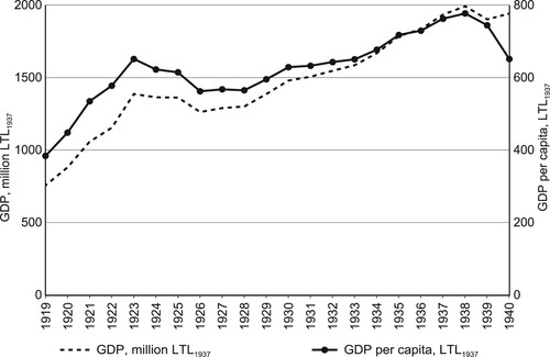
However, by 1924, the Lithuanian economy had started to decline, and was particularly damaged by the recession of 1926–1928, which has not been widely discussed on an international level, although it was also evident in Estonia. The underlying causes of this downturn, which was most prominent in the industrial sector, remain to be explored thoroughly by future scholars.

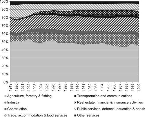
The period following 1928 witnessed a gradual but modest economic growth, leading to a 46% overall increase in GDP and a 25% increase in per capita income between 1924 and 1938. The average annual growth rate during this period was only 2.8%, which is considerably lower than the previously assumed rate of 4.8% (Vaskela, 2015, p. 328). Contrary to several previous studies (see Prekybos, pramonės ir amatų rūmai, 1938; Vaskela, 2005, p. 486), there was no significant industrial transformation in Lithuania the 1930s. As shown by Figure 4, the industry's contribution to GDP grew at a slow pace (from 12.5% in 1924 to 14.5% in 1938) and even declined after the loss of Klaipėda region in 1939. At the time of the Soviet invasion in 1940, Lithuania remained predominantly an agricultural economy.

Figure 4. Structure of Lithuanian gross value-added at constant prices, 1919–1940. SOURCE: calculations in this paper.

The lack of robust growth and slow industrialisation can be attributed to the unsuccessful import-substitution strategy perfected by Denmark before World War I (Berend, 2006, p. 29), which was challenging to replicate in the declining global trade terms of the inter-war period. The prevailing belief was that Lithuania could sustain itself by exporting food (Vygandas, 1930, p. 47) and potentially use the proceeds from trade to promote internal industrialisation. This notion changed only after the global trade contraction of the 1930s (Vaskela, 2015, pp. 298–299).

The agricultural sector, thought to have grown by about 3.5–4% annually (Vaskela, 2005, p. 488), was also stagnant. The newly compiled data indicates an annual growth rate of only 2.1% between 1924 and 1938, which is in line with the consensus of global agricultural oversupply that caused a contraction in the sector (Kindleberger, 1986, p. 73). It is worth examining the structural changes in the value-added of agriculture during this period. According to Povilaitis (1988, p. 277), who based his conclusion on export data, the primary sector in Lithuania gradually shifted from crop production to livestock during the inter-war period. However, Table 6 does not reveal any clear pattern of transition away from crop production. The lowest crop-to-livestock value-added ratio was observed during the post-World War I recovery phase (as shown in Table 6), which could be attributed to the physical devastation of land resulting from the Great War and the struggle for independence. Furthermore, when international trade contracted after 1929 and Lithuanian processed food exports declined, farmers appeared to have slightly shifted back towards crop cultivation.

Table 6. Ratio value-added of crops to livestock 1920–1938.

Period	Crops to livestock VA ratio	Comment
1920–1922	0.59	Post-war recovery
1923–1929	0.61	Pre-crisis stagnation
1930–1935	0.69	Great Depression
1936–1938	0.63	Post-crisis growth

Source: calculations in this paper. For details see Appendix 2. 1919 and 1939–1940 are excluded due to structural breaks caused by major territorial changes.

In terms of its overall structure, the Lithuanian economy remained largely unchanged throughout the inter-war period (see Figure 4). While the share of agriculture in the economy experienced a steady but slow decline, there was some growth observed in the industrial sector. However, the shares of other sectors remained stagnant. This is not surprising, as services such as trade and transportation mainly served the primary and secondary sectors, and the combined share of both these sectors remained nearly constant.

Steady economic growth was disrupted by the loss of Klaipėda region in March 1939, which was partially offset by the incorporation of the underdeveloped Vilnius area in October 1939. Despite this, the total GDP figure for 1939 still fell, as Lithuania only possessed Vilnius for the last two months of that year. The full impact of the territorial expansion was felt in 1940, resulting in an overall increase in GDP. However, due to the corresponding population rise, the war in Europe, and the Soviet occupation, per capita income in Lithuania sharply declined. Additionally, the harsh winter of 1940 further worsened the downturn in agricultural value-added, despite the 1/6 territorial increase.

Strikingly, the stagnant Lithuanian economy withstood the Great Depression without a single year of negative growth. Its poor foreign trade performance suggests some preliminary explanation. According to Table 7, Lithuania had one of the lowest trade-to-GDP ratios in Europe in 1929, even lower than Italy, which aimed for complete self-sufficiency (Berend, 2006, pp. 100, 116). Hence, it is possible that the isolated Baltic state was not impacted by the global contraction to the same extent as its peers. By 1938 Lithuania's trade-to-GDP ratio had recovered which is again in contrast to other countries. This is a highly unconventional pattern for a country which remained fully committed to the gold standard until 1935.¹³

Table 7. Trade (imports plus exports) to GDP ratios in selected countries in 1929 and 1938.

Country	1929	1938
Czechoslovakia	52%	no data
Finland	50%	44%
Estonia	47%	38%
UK	40%	24%
Sweden	37%	31%
Italy	25%	15%
Lithuania	24%	23%

Source: calculations in this paper, foreign trade data from League of Nations Economic Intelligence Service (1940, pp. 182–187) and GDP data from Baffigi (2011, pp. 18, 24), Valge (2003, p. 2719), Hjerppe (1996, p. 102), Williamson (2023), Edvinsson (2014) and Stádník (1968, p. 30). Lithuanian imports and exports deflated to 1937 prices using the general price index from Table 2.

The purpose of this paper is not to explore in depth why the Lithuanian economy proved to be so resilient during the inter-war period. However, this raises intriguing questions about the effectiveness of expansionist policies, which were once again implemented in response to the pandemic of 2020. By choosing not to devalue its currency, Lithuania limited its ability to introduce recovery policies and was forced to see the competitiveness of its exports decline. Nevertheless, this had only a negligible impact on its GDP. If a small agrarian economy was able to weather the worst financial crisis of the modern era by pursuing a deflationary course, it suggests that perhaps modern underdeveloped states might benefit from a similar approach. With the help of the datasets constructed in this paper, future research can hopefully shed light on these questions.

In a broader European context, inter-war Lithuania was a typical average-performing periphery (see Figure 5). In contrast to Vaskela (2015, p. 330) the country only slightly converged towards Estonia, failing to catch up with the West and Finland. Longer-run statistical comparisons provide a more curious perspective. Judging from Table 8, countries that have emerged on the map of Europe after WW1 have seen both convergent and divergent trends in GDP per capita. By 1938 the Baltic states had improved their positions relative to Austria, Finland and the Central European economies. However, in the post-WW2 years, while overtaking the per capita income levels of the sovereign communist states of Europe, the Baltic Soviet republics fell further behind the capitalist Austria and Finland. Since the collapse of the Communist bloc, all three groups have been reconverging towards each other.

Figure 5. Level of Lithuanian GDP per capita in GK$₁₉₉₀ as percentage of other countries. SOURCE: calculations of this paper, Valge (2003, pp. 2726–2727) and Bolt et al. (2018). The GDP per capita of the post-WW1 emerging states aggregated by dividing the sum of total GDP of those countries by the sum of respective total populations. Western European data taken from Bolt and van Zanden (2014) and includes Austria, Belgium, Denmark, Finland, France, Germany, Italy, Netherlands, Norway, Sweden, Switzerland and the UK.

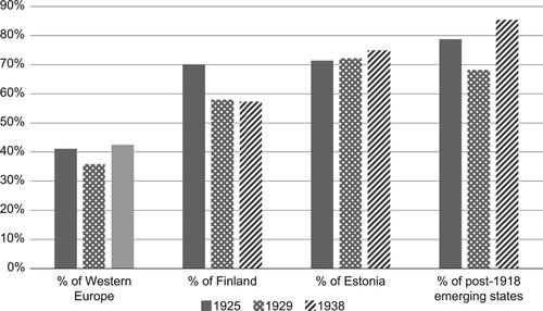
Table 8. Divergence of GDP per capita in post-WW1 emerging states, Group 3 = 100.

	1922	1929	1938	1973	1990	2019
Group 1	164	170	145	142	178	153
Group 2	96	110	90	69	63	94
Group 3	100	100	100	100	100	100

Source: calculations of this paper, Valge (2003, pp. 2726–2727), Bolt et al. (2018), and Bolt and van Zanden (2020). Group 1: Austria and Finland. Group 2: Poland, former Czechoslovakia, Hungary, former Yugoslavia. Group 3: Lithuania, Latvia and Estonia.

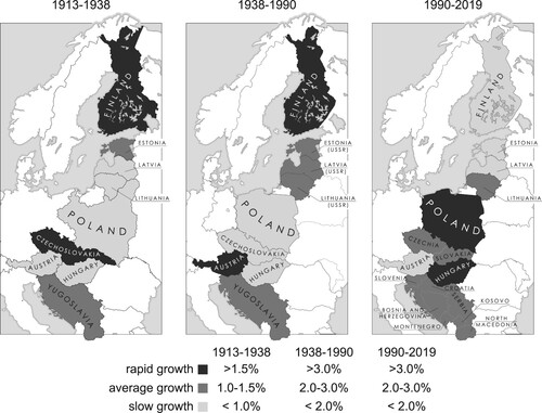
Additional gaps in East-Central European GDP map need to be filled before a comprehensive analysis of the 20th century growth in the region can be performed. Nevertheless, some new implications can already be drawn about its regional development using the new data. The inter-war was a period of slow growth across Europe, in stark contrast to the post-WW2 era when economies advanced at unprecedented levels throughout the continent (Feinstein et al., 1997, p. 188). Lithuania and most of the East-Central Europe were not exceptional in this, as Figure 6 indicates. While it has already been argued that rapid growth in the region was only achieved during the Cold War years (Klimantas & Zirgulis, 2020, p. 254), the evidence suggests that Soviet-occupied underdeveloped parts of Europe experienced larger economic booms than the communist satellites such as Poland or Hungary. However, The Baltic states also saw catastrophic recessions following the collapse of the USSR and transitioning back to capitalism. The slump was markedly less evident among the former sovereign communist states. In fact, the post-Soviet recession in the Baltics was so severe compared to the rest of the former Communist Europe, that by 1995 the levels of income per head in the two groups of countries had equalised. The Soviet occupation led to industrialisation and a surge in income levels, but the USSR's dependence on its flawed internal system and lack of competitiveness proved the fleeting nature of these gains after the 1990s crash.

Figure 6. Compound annual GDP per capita growth rates in post-WW1 emerging states. Source: calculations of this paper, Valge (2003, pp. 2726–2727), Bolt et al. (2018), Bolt and van Zanden (2020), and Norkus and Markevičiūtė (2021, p. 603).

4. Conclusion

This paper pioneers the use of the benchmark extrapolation approach to the historical national accounts in the Baltics. By producing constant-price sectoral growth aggregates, the study was able to estimate the GDP and GDP per capita time series in Lithuania from 1919 to 1940. The database of the previously non-existent main sectoral aggregates is useful on its own. And although the figures are subject to improvement, the cross-checked GDP series sheds new light on Lithuania's inter-war performance until its incorporation into the USSR. The figures indicate that Lithuania was an isolated, stagnating European periphery, but with comparatively high resilience towards the Great Depression.

The paper also opened inter-war Lithuania for international comparisons by converting the GDP per capita series into international Geary-Khamis dollars. These figures, along with the mean annual population statistics, can now be integrated into international databases such as the Maddison project for worldwide use.

Although today Lithuania remains a small economy with few international applications for its long-run GDP trends, the three Baltic states offer a joint story of successful transitions between capitalism and planned economy worth analysing. However, income levels of Soviet-occupied Lithuania, Latvia, and Estonia before 1980 are still unknown. Future studies will fill these gaps, allowing for a full examination of East-Central Europe's unique long-run development from 1918 through the Great Depression, post-war growth, pre-1990 stagnation, successful transition to a market system and the ongoing convergence towards the West.

Disclosure statement

No potential conflict of interest was reported by the author(s).

Additional information

Funding

The author acknowledges financial support from the Baltic Research Programme project ‘Quantitative Data About Societal and Economic Transformations in the Regions of the Three Baltic States During the Last Hundred Years for the Analysis of Historical Transformations and the Overcoming of Future Challenges’ (BALTIC100), project No. EEA-RESEARCH-174, under the EEA Grant of Iceland, Liechtenstein and Norway Contract No. EEZ/BPP/VIAA/2021/3.

Notes

1 The authors used the indirect estimation procedure employed in the 2018 Maddison Project issue (see Bolt et al., 2018).

2 There is only one single-year limited family budget study (Centralinis Statistikos Biuras, 1939e).

3 It should be noted that estimates are provided in GK$₁₉₉₀ only as the first attempt at comparability. While following the Maddison project PPP conversion framework, this paper acknowledges its flaws and encourages further research to provide additional comparability measures.

4 The region was part of Germany until 1919, inhabited by mixed Lithuanian-German population.

5 These were annual surveys of samples of small, medium and large farms carried out with increasing sample sizes since 1932.

6 In 1921 Lithuania received a coastal strip on the Baltic shore, in 1923 the whole seaside Klaipėda region came under its control and in 1939 this region was lost.

7 Reporting was inconsistent and provided a false sense of immense growth due to gradual expansion of the number of enterprises which provided data for CSB. Therefore, industrial production index compiled by the House of Commerce, Industry and Crafts (Prekybos, pramonės ir amatų rūmai, 1938) using CSB data is misleading.

8 As late as in 1940, land freight ton-km was just 13 thousand compared to 441,100 thousand in railways. See Table A5 and Meškauskas (1960, p. 237).

9 See Appendix 1.

10 With an upward amendment by 1.4% suggested by Norkus et al. (2022, p. 71).

11 The Estonian GDP data (Valge, 2003) is very limited in scope, covering only a few sectors, while Iceland's most relevant historical GDP study (Jonsson, 1999) closely resembles the latest efforts in Lithuania and Latvia. Jonsson employed a combination of output and income approaches, encountering challenges related to data scarcity similar to this paper. For instance, to cover the manufacturing sector, employment data from various subsectors were aggregated using 1934 income data. However, Icelandic primary sector series are double-deflated, enhancing the quality of the estimates. The Latvian inter-war GDP study, published in parallel with the current study (Klimantas et al., 2023, august), closely mirror the benchmark extrapolation with single deflation approach employed in this paper with almost identical data situation. The Danish series rely on the 1972–1974 study by Svend Aage Hansen, summarised in Christensen et al. (1995, pp. 39-40). These series are constructed at current prices without double deflation but with better data coverage than Estonian, Icelandic or even the latest Latvian and present Lithuanian studies. In contrast, the superior Finnish, Swedish, and Norwegian series benefit from significantly broader data availability compared to their Baltic counterparts. Methodologically, the Finnish series by Hjerppe (1989) continue to adopt single deflation but introduce multiple benchmarks every decade. In Sweden's case, where the HNA series have undergone substantial revisions, Edvinsson (2013b) dismissed double deflation in favour of unchanging value-added shares, subsequently correcting for structural changes in the long run. Likewise, while earlier efforts by Krantz and Schön (2007) employed double deflation, their subsequent work (Schön & Krantz, 2012) shifted to single deflation, utilising different deflators (Fisher instead of Paasche). Finally, the Norwegian historical GDP firmly rely on double-deflated series, which have been continuously enhanced (see Grytten, 2021, 2022).

12 It was previously thought that Lithuanian national income doubled and per capita incomes increased by ∼75% during 1924–1938 (see Meškauskas et al., 1976, p. 410; Vaskela, 2014, p. 86)

13 Empirical evidence from the West strongly supports the notion that the gold standard is susceptible to transmitting economic shocks (see Bernanke & James, 1990, p. 33), and devaluation typically results in output recovery in the majority of cases (see Eichengreen & Sachs, 1985, p. 934).

14 The only exception is 1919 for which only tax data is available. The tax, however, was levied according to the certificate category an enterprise belongs to, allowing to connect 1919 figure with the rest of the period data.

15 Following the invasion, in 1940 Soviet officials forced all craftsmen into factories, providing full industrial workforce numbers.

16 The paper follows the assumption by Allen (2001, p. 414) that construction worker wages are representative of all unskilled workers.

Appendices

Appendix 1.

Improvements in benchmark GDP

This section provides an overview of the improvements to the Klimantas and Zirgulis (2020) 1937 benchmark made in this paper. Firstly, the distributive trade VA is moved from the transportation to the trade sector. Secondly, the real estate output is recalculated. Klimantas and Zirgulis (2020, p. 268) used the real estate ‘taxable base’ as the main output entry. This is misleading as the tax had to be paid on the property owned rather than actually leased (Micuta, 1930/1990, p. 183). This paper managed to obtain data on rental incomes and intermediate consumption of property developers in Kaunas (capital city) from 1932 (Valdininkas, 1932, february 18). Thus, VA in 1932 is reconstructed, reflated by the cost of living index, multiplied by entire urban to Kaunas city population ratio to arrive at the constant-price VA of real estate activities in 1932. Using an index compiled in Section 2.2.6, 1937 VA of 90.75 million LTL is obtained. Adding up the government real estate activities from Klimantas & Zirgulis gives a total VA of 92.94 million LTL in 1937. As there is no data on brokerage firm operations and rural real estate activities are covered by undifferentiated household income in ‘Other services’, this figure is assumed to represent the entire Lithuanian commercial real estate activity. Thirdly, private healthcare activities are included using a 1.6 ratio of total to public hospital beds (Centralinis Statistikos Biuras, 1938a, p. 57). This results in the healthcare VA of 8.2 million LTL instead of 5.1 million. Thirdly, value-adding activities of households (ISIC sector T) from the benchmark study are expanded to include the rural household crafts and other activities from the Agricultural survey results (Žemės Ūkio Rūmai, 1940, p. 39). This results in a total of 39.7 million LTL attributed to the activities of households as employers/undifferentiated household income in ‘Other services’.

Finally, the GK$1990-to-LTL1937 PPP conversion ratio was increased by 1.4% to 2.647 as suggested by Norkus et al. (2022, p. 71). The amendment was needed as there was a slight mistake in the benchmark study.

Appendix 2.

Estimation of sectoral volume indices

This appendix presents the details of volume index construction of all sectors included in GDP estimation in this paper. As a rule, value-added series are obtained by multiplying series obtained from sources listed below by the revised benchmark value-added (VA) figures.

A.1. Crops

In estimating VA of crops, indices of physical yields of rye, wheat, barley, oats, peas, linseed, flax fibre, potatoes and sugar beet are multiplied by 1937 output figure from Klimantas & Zirgulis using the composition of output weights from Agricultural survey results. This paper assumes that ‘Other crops’ figure moved together with the rest of the additive crop output index. Constant GK$₁₉₉₀-to-LTL₁₉₃₇ ratio from 1937 is used to arrive at constant-price VA series. See Table A1 for data and sources.

Table A1. Output and value-added of crops, million LTL in 1937 prices.

Year	Rye	Wheat	Barley	Oats	Peas	Linseed	Flax fibre	Potatoes	Sugar beet	Other crops	Total output	VA of crops
1919	56.4	19.2	8.6	5.8	3.0	5.4	24.1	9.9	0.0	48.6	181.0	162.7
1920	54.5	16.0	7.5	5.3	2.3	6.6	22.4	14.2	0.0	47.4	176.4	158.6
1921	68.8	20.6	9.3	6.8	3.6	6.0	20.4	15.4	0.0	55.4	206.3	185.4
1922	79.2	23.8	14.9	10.9	5.3	7.3	18.7	20.5	0.0	66.4	246.9	222.0
1923	77.9	21.5	11.0	8.6	4.4	6.9	30.1	18.1	0.0	65.6	244.2	219.5
1924	59.8	24.1	12.9	8.7	5.3	8.7	32.5	18.4	0.0	62.7	233.1	209.6
1925	85.3	38.4	15.6	7.8	5.0	10.1	29.0	17.6	0.0	76.7	285.5	256.7
1926	46.7	27.2	12.8	10.2	3.7	10.7	38.8	14.7	0.0	60.6	225.5	202.7
1927	66.0	41.2	11.0	9.1	4.3	9.3	33.5	12.2	0.0	68.6	255.4	229.6
1928	61.7	47.0	9.6	9.8	3.7	6.1	32.3	10.7	0.0	66.5	247.4	222.4
1929	76.5	56.3	15.1	15.3	5.9	11.4	34.3	20.4	0.0	86.4	321.4	289.0
1930	85.9	65.6	12.9	14.2	5.9	10.0	28.8	19.5	0.0	89.3	332.1	298.6
1931	53.0	60.5	15.4	14.0	5.8	6.6	21.1	21.5	3.5	74.1	275.5	247.7
1932	73.6	68.4	15.2	12.1	5.0	4.1	14.2	21.3	8.9	81.9	304.8	274.0
1933	71.0	59.9	14.8	11.4	5.2	5.6	18.8	20.3	7.5	78.8	293.3	263.6
1934	86.3	76.0	16.2	13.0	3.6	6.8	22.1	27.0	6.9	94.8	352.8	317.1
1935	82.4	73.2	16.0	13.6	4.1	9.8	31.8	19.7	10.3	95.9	356.7	320.7
1936	69.8	58.2	14.9	11.3	3.8	9.5	29.0	23.5	13.3	85.7	318.9	286.7
1937	78.1	58.8	17.5	13.2	2.8	9.2	31.2	27.9	14.5	93.1	346.2	311.2
1938	80.2	67.0	17.5	14.3	4.0	7.6	25.7	23.5	11.2	92.3	343.3	308.6
1939	92.9	69.5	17.1	14.9	4.7	8.5	29.1	26.1	13.3	101.5	377.6	339.4
1940	79.4	47.0	14.2	11.4	3.7	7.5	30.5	30.0	19.9	89.5	333.0	299.4

Sources: Crop yields from Centralinis Statistikos Biuras (1927, pp. 146–147), Centralinis Statistikos Biuras (1938a, pp. 127–133), Musteikis (1948, p. 208), Žemės Ūkio Ministerija (1940, p. 12), and A review (1923, p. 4). Crop weights in output from Žemės Ūkio Rūmai (1940, pp. 37–39). Output and VA 1937 figures from Klimantas and Zirgulis (2020, p. 256). Oats were reported together with meslin (used for fodder) until 1925. Data is separated using 1926–1940 ratio.

A.2. Livestock

In the livestock sector, physical output series of milk, beef and other cattle output, pigs, sheep, eggs, horses and other livestock production are compiled and aggregated into a single index in the same way as with crops (sources in Table A2). In the case of milk, the annual number of milk cows is multiplied by the annual output of milk per cow. Output per cow is only available 1926 and 1939, being 700 kg and 1964 kg respectively. This paper assumes no change in 1919–1926 (probable given pre-WW1 milk production was ∼750 kg per cow (Paltarokas, 1968, p. 185)) and in 1939–1940. Output for 1927–1938 is interpolated.

Table A2. Output and value-added of livestock million LTL in 1937 prices.

Year	Milk	Other cattle	Pig farming	Sheep farming	Egg production	Horse farming	Other livestock	Total output	VA of livestock
1919	23.1	12.8	115.5	13.2	9.2	12.7	21.0	207.5	198.8
1920	30.8	16.5	170.5	14.6	9.2	15.1	28.9	285.8	273.8
1921	37.6	19.3	193.6	17.0	12.7	17.0	33.5	330.7	316.9
1922	46.0	24.1	216.7	19.5	14.4	19.0	38.3	378.0	362.2
1923	61.9	30.1	243.4	23.1	14.0	22.8	44.5	439.9	421.4
1924	60.3	28.9	241.6	23.2	14.1	21.8	43.9	433.9	415.7
1925	64.5	29.3	223.8	21.7	14.0	20.9	42.2	416.5	399.0
1926	67.3	32.9	216.7	25.6	15.4	32.6	44.0	434.6	416.4
1927	61.9	29.7	165.2	24.0	16.3	32.3	37.1	366.6	351.2
1928	72.5	32.5	165.2	25.5	17.5	29.2	38.6	381.1	365.1
1929	80.6	32.1	145.7	18.5	18.2	24.9	36.1	356.1	341.2
1930	83.7	29.3	165.2	19.9	19.4	25.1	38.6	381.2	365.2
1931	96.7	33.7	177.6	22.5	21.0	27.9	42.8	422.2	404.5
1932	109.6	39.3	170.5	22.3	21.3	26.5	43.9	433.6	415.4
1933	119.1	37.7	181.2	20.8	21.6	24.4	45.6	450.4	431.5
1934	127.4	40.5	181.2	21.2	22.3	23.3	46.9	462.8	443.4
1935	139.2	40.1	181.2	22.2	24.2	21.8	48.3	477.1	457.1
1936	150.2	39.3	181.2	21.9	28.0	22.3	49.9	492.8	472.2
1937	159.1	40.1	177.6	23.5	28.8	24.2	51.1	504.5	483.4
1938	170.9	40.1	186.5	23.7	29.8	24.8	53.6	529.5	507.3
1939	188.1	39.3	181.2	23.7	30.4	25.4	55.0	543.0	520.3
1940	171.9	32.5	179.4	24.5	33.0	23.1	52.3	516.8	495.1

Sources: Livestock numbers from Lietuvos žemės ūkis (1922, p. 5), Rimka (1926a, p. 72), Centralinis Statistikos Biuras (1931, pp. 176–177), Centralinis Statistikos Biuras (1933, pp. 78–81), 78–81, Centralinis Statistikos Biuras (1937a, pp. 80–81), Centralinis Statistikos Biuras (1938c, p. 3), and Musteikis (1948, p. 209). Milk per cow from Moravskis (1913–1938c) and Klupšas (2008, p. 789).Proportions of slaughtered animals from Centralinis Statistikos Biuras (1929a, p. 65) and Centralinis Statistikos Biuras (1940a, p. 115).Export data from Centralinis Statistikos Biuras (1923, p. 186), Centralinis Statistikos Biuras (1927, priedas 1, p. X–XVI), Centralinis Statistikos Biuras (1929b, priedas 8), Centralinis Statistikos Biuras (1940a, pp. 114, 244, 281), Centralinis Statistikos Biuras (1929a, p. 91), Moravskis (1913–1938c), Žemės Ūkio Ministerija (1940, p. 60), Centralinis Statistikos Biuras (1930, pp. 1–2), Centralinis Statistikos Biuras (1932b, pp. 1–2), Centralinis Statistikos Biuras (1934, pp. 1–2), Centralinis Statistikos Biuras (1935b, pp. 1–2), Centralinis Statistikos Biuras (1936b, pp. 1–2), Centralinis Statistikos Biuras (1937b, pp. 1–2), Centralinis Statistikos Biuras (1938b, pp. 1–2), Centralinis Statistikos Biuras (1939b, pp. 1–2), and Centralinis Statistikos Biuras (1940c, p. 70).Animal weights and basic prices from Maistas AB (1933, pp. 69–72), Maistas AB (1933, p. 9), Maistas AB (1934, p. 7), Maistas AB (1935, p. 7), Maistas AB (1936, p. 7), Maistas AB (1937, p. 8), Maistas AB (1938, p. 27), Maistas AB (1939, p. 10), Maistas AB (1940, p. 6), and Maistas AB (1941).Wool output from Meškauskas and Meškauskienė (1972, p. 28).Consumption of eggs from Rimka (1926b, p. 107), Musteikis (1948, p. 209), and Klupšas (2008, p. 790).Separate livestock production weights in output from Žemės Ūkio Rūmai (1940, pp. 37–39).Output and VA 1937 figures from Klimantas and Zirgulis (2020, p. 256).Note: in case of missing data, unavailable numbers are extrapolated from related data if possible. If not, constant pre-crisis or post-crisis averages assumed for longer periods and nearest year data for single missing years (e.g. 1940).

Other cattle output consists of the value of animals slaughtered by farmers plus sales for slaughter or export (including the value of hides). Total weight of such animals is obtained from proportions of slaughtered and exported animals multiplied by average annual weights of respective cattle (bulls and calves). These series are joined using basic prices of calves and bulls.

As with cattle, pig production is estimated from the proportion of animals sold for slaughter or export, adjusted for weight changes. Slaughter- or export-bound sheep output is estimated in the same way. With regards to wool production, the annual output of 1.15 kg per sheep from 1937 is used. That is the only figure available. Multiplying it by the annual number of sheep yields a series of wool output (it falls well inside approximate output range quoted by Povilaitis, 1988, p. 144). Basic prices per kg of slaughter-bound sheep and wool are used to create a joint index of sheep production.

Egg production index is compiled from consumption and export data. Consumption figures are only available for 1924 and 1936–1939. The 1924 figure of 65 eggs per capita comes from ‘minimum existential consumption’ and is thus assumed to be the same in 1919–1923, 1925–1935 figures are interpolated and 1940 is assumed to have brought no change from 1936–1939 average (152 eggs per capita). The total number of eggs are obtained by multiplying per capita averages by population and adding up exported eggs. A 1930–1939 cross-check with the number of chicken yielded almost identical series.

Horse growing activities in Agricultural accounting survey includes both sales of horses and hide output. Assuming a constant number of working horses, the series of horse sales is approximated by changes in numbers of offspring horses. Such data is available since 1925. The full index is obtained by applying the post-1925 proportion of young to mature horses for 1919–1924.

Changes in the output of other livestock are taken from 1932–1938 Agricultural accounting survey results, reflated by the agricultural price index. It is assumed that during the years 1919–1931 and 1938–1940 other livestock followed the overall trend of the livestock sector.

Potential upward bias in agricultural output is worth noting (see Table 5). In 1930s CSB revised some of its earlier crop yield and animal stock figures following the 1930 agricultural census. However, 1919–1924 figures remained untouched and thus are subject to overestimation.

A.3. Forestry, fishing and primary sector totals

Physical amounts of forest material sold are available for entire 1919–1940 period. These are, however, figures of state forest material sales, while no data for private ones (19% of total forests Centralinis Statistikos Biuras, 1939a, p. 144) exists. It is thus assumed that private forestry moved together with the public one.

Lithuania's total physical fishing output data exists from 1933 to 1940 and the period 1923–1932 is covered by data from the seaside Klaipėda region. No data for the years before to 1923 is available. 1939–1940 figures represent fishing output in Lithuania without Klaipėda region. Ratio Klaipėda region to whole Lithuania‘s output fluctuated around 0.6 between 1933 and 1938. This ratio is used to estimate the whole Lithuania‘s fishing output between 1923 and 1932. For 1919–1920 and 1921–1922, figures are assumed to be the same as was in 1933–1939 in the respective territory. Indices for both forestry and fishing are compiled accordingly and multiplied by VA figure in Klimantas and Zirgulis (see Table A3).

Table A3. Value-added of primary sector, million LTL in 1937 prices.

Year	Crops	Livestock	Forestry	Fishing	Total
1919	162.7	198.8	3.1	0.23	364.9
1920	158.6	273.8	5.0	0.23	437.6
1921	185.4	316.9	9.0	0.46	511.8
1922	222.0	362.2	11.9	0.46	596.5
1923	219.5	421.4	15.8	2.31	659.1
1924	209.6	415.7	10.0	2.42	637.6
1925	256.7	399.0	14.1	2.44	672.3
1926	202.7	416.4	10.4	2.07	631.5
1927	229.6	351.2	17.3	1.64	599.7
1928	222.4	365.1	19.4	1.33	608.2
1929	289.0	341.2	18.0	1.53	649.6
1930	298.6	365.2	15.6	1.50	680.9
1931	247.7	404.5	19.2	1.65	673.1
1932	274.0	415.4	18.1	1.68	709.2
1933	263.6	431.5	23.6	1.38	720.2
1934	317.1	443.4	20.0	1.20	781.8
1935	320.7	457.1	20.9	1.09	799.8
1936	286.7	472.2	28.9	1.07	788.8
1937	311.2	483.4	27.3	1.08	823.0
1938	308.6	507.3	25.0	1.14	842.1
1939	339.4	520.3	20.5	0.55	880.8
1940	299.4	495.1	28.1	0.52	823.2

Source: Tables A1 & A2 and Žemės Ūkio Ministerija (1940, p. 303), Centralinis Statistikos Biuras (1940a, p. 136), and Centrinė Statistikos Valdyba (1960, p. 112) for forestry and Moravskis (1938e), Moravskis (1913–1938d), Centralinis Statistikos Biuras (1929b, pp. 201–205), Centralinis Statistikos Biuras (1931, pp. 192–193), Centralinis Statistikos Biuras (1935a, p. 93), Centralinis Statistikos Biuras (1937a, p. 101), Centralinis Statistikos Biuras (1939a, p. 141), Centralinis Statistikos Biuras (1940a, p. 131), and Centrinė Statistikos Valdyba (1960, p. 130) for fishing.

A.4. Industry

Employment data used in this paper to estimate the movement of the industrial sector mainly comes from the number of workers in the largest enterprises reported since 1926. Pre-1926 whole employment figures and post-1926 small enterprise employment figures are estimated from industrial certificate data. Industrial enterprises in inter-war Lithuania had to obtain certificates according to the number of workers they have and the machinery they own. Therefore, the average numbers of workers in each certificate category were multiplied by the number of enterprises in the respective category to arrive at the number of workers.¹⁴ A cross-check with 1940 (Centrinė Statistikos Valdyba, 1960, p. 282)¹⁵ total number of industrial workers data provides great confidence in such procedure (62,300 versus 63,210 obtained in this study). To account for worker productivity change, real wages of industrial workers are used for 1930–1940 period and those of construction workers¹⁶ for 1924–1929 period. Due to data constraints, an assumption is made that there were no productivity gains between 1919 and 1924, except for adjustment for industrially more productive Klaipėda region's inclusion in 1923. The assumption seems reasonable as during the recovery phase in 1919–1923 all productivity gain was likely reflected in the increase in the number of workers. VA is obtained by multiplying the resulting workforce index by VA figure from the benchmark study. Data is presented in Table A4.

A.5. Construction

Regarding housing construction, the number of houses built is used for 1922–1932, cubic volume for 1937–1939, deflated monetary value of capital invested for 1933–1936 and urban/rural population change for 1919–1921 and 1940. To obtain monetary constant-price series, average capital investments in residential and non-residential (urban and rural) housing are taken from 1937 Statistical yearbook.

In case of infrastructure projects (railroads, roads, bridges, waterways and communication lines), there are no consistent physical series to account for these activities. Therefore, the deflated monetary series of respective construction spending are used. Separate figures are available in statistical yearbooks since 1932. Earlier year figures are extrapolated using the change in extraordinary expenditures by the Ministry of Transport and Communications (86% of which were construction expenditures Valstybės kontrolė, 1938, pp. 214–221). The resulting infrastructure project series was deflated using the construction material price index from Table 2. Data and full sources used for industrial and construction calculations can be found in Table A4.

A.6. Trade and accommodation & food service activities

As mentioned in the main text, the change in the value-added of trade is a function of the change in the value added of agricultural and industrial goods which were actually sold in the market. For this it was necessary to estimate the share of crops, animal, forest production, fish, industrial goods and imports that were sold in the market versus the share consumed by the producers themselves. In the case of agricultural goods, the proportion of home-used/marketed production is obtained from Agricultural accounting survey results (Žemės Ūkio Rūmai, 1934, p. 33 and Žemės Ūkio Rūmai, 1940, pp. 56–58). They indicate that average share of production marketed was 58% with crops and 56% with livestock in 1932–1934. There was a tendency for the share of crops marketed to rise, while the respective livestock proportion was generally stable. Thus, the ratio from 1932–1933 for crops before 1934 and the ratio from 1934–1937 for the rest of the period is used. With livestock, 56% ratio is employed for the entire inter-war period. Finally, 100% of forestry, fishing, industrial and imported goods are assumed to have reached the market. Absolute marketed values of all mentioned goods are aggregated to arrive at trade VA index which is multiplied by the VA of the trade from benchmark data. Sources presented in Table A5.

A.7. Transportation and communications

With regards to railway transportation, passenger-km and ton-km data are available for entire 1919–1940 period. Land transportation passenger-km is available only for 1933–1940 period, showing signs of growing popularity towards the end of the decade. This paper uses the number of buses (1927–1932) and population growth (1919–1926) to extrapolate land transportation series. Weight of goods transported via marine and inland transport figures are available for the entire inter-war period, as with communications services data. For sources and data series see Table A5.

A.8. Financial, insurance & real estate activities (FIRE)

Bank deposit statistics are available for entire 1919–1940 period. Loan data only begins in 1922. 1919–1921 loan data is extrapolated using the loan/deposit ratio from later periods. In cases of early data, only the largest credit institutions are documented. This issue is solved by applying ratios of total deposits/loans to large bank deposits/loans from later periods. Annual interest rates on loans and deposits are used to obtain the output of banking. There are gaps in interest rate data which are filled by interpolation. Data on insurance premium is available for 1928–1939. Insurance is assumed to have moved together with financial services for the rest of the inter-war. Benchmark VAs are taken from Klimantas and Zirgulis (2020).

The only option for tracking change in RE activity in inter-war Lithuania is through real estate tax receipts. The tax rate changed in mid-1935 and in late 1939 (which is irrelevant because tax data for 1940 is unavailable). Using relevant tax rates, ‘taxable base’ figure is obtained and deflated by the cost of living index from Table 2. The resulting index is multiplied by benchmark VA from Appendix 1. VA series and sources of the FIRE sector are presented in Table A6.

Table A4. Value-added calculations of industry and construction, 1937 = 100 for indices, LTL₁₉₃₇ for monetary values.

Year	Number of workers	Worker productivity index	Industrial production index	VA of industry, million LTL	Housing construction index	Infrastructure construction index	Joint construction index	VA of construction, million LTL
1919	19,591	68	22	61.0	61	1	48	32.9
1920	15,227	68	17	47.5	61	4	49	33.2
1921	29,665	68	33	92.4	62	5	49	33.5
1922	30,060	68	33	93.7	62	3	49	33.7
1923	46,520	83	63	175.3	96	24	80	54.6
1924	45,370	83	61	170.9	121	20	99	67.3
1925	45,070	65	48	134.6	111	27	93	63.4
1926	40,473	64	42	117.4	100	10	80	54.7
1927	44,187	72	52	146.1	111	12	90	61.3
1928	44,275	62	45	125.4	124	17	100	68.4
1929	44,863	70	51	143.7	106	16	86	58.8
1930	43,360	83	59	163.7	119	44	103	70.1
1931	46,025	85	64	178.2	120	46	104	70.7
1932	43,188	94	67	186.1	93	71	88	60.1
1933	44,439	93	68	189.2	98	65	91	61.8
1934	47,902	90	70	197.0	69	53	65	44.5
1935	48,756	104	83	231.3	69	66	69	46.8
1936	55,129	102	92	256.9	94	61	87	59.5
1937	61,274	100	100	279.7	100	100	100	68.2
1938	64,262	98	103	287.8	107	110	108	73.7
1939	57,021	81	75	210.5	117	100	113	77.4
1940	63,210	79	82	228.5	154	100	142	96.8

Source: Industrial worker numbers from Centralinis Statistikos Biuras (1939c, p. 96), Centralinis Statistikos Biuras (1936a, p. 203), Centralinis Statistikos Biuras (1940a, pp. 160–161), Meškauskas et al. (1976, p. 457), 457, and Meškauskas and Meškauskienė (1980, p. 17). Industrial certificate data from Šalčius (1956, pp. 248–249), Centralinis Statistikos Biuras (1931, pp. 250–253), Centralinis Statistikos Biuras (1933, p. 178), Centralinis Statistikos Biuras (1936a, p. 221), Centralinis Statistikos Biuras (1940a, p. 191), and Centralinis Statistikos Biuras (1940d, p. 95). 1919 tax data from Micuta (1930/1990, pp. 180–182). Mean number of workers per certificate category from Centralinis Statistikos Biuras (1929b, pp. 211–216), Centralinis Statistikos Biuras (1931, p. 241), and Fridbergas (1988, pp. 34–35); Worker wages from Centralinis Statistikos Biuras (1940a, p. 188), Centralinis Statistikos Biuras (1940b, p. 36), Centralinis Statistikos Biuras (1940f, p. 159), and Norkus and Markevičiūtė (2021, p. 652). Housing construction data from Centralinis Statistikos Biuras (1929b, p. 232), Centralinis Statistikos Biuras (1931, pp. 276–277), Centralinis Statistikos Biuras (1932a, pp. 165–166), Centralinis Statistikos Biuras (1933, pp. 203–207), Centralinis Statistikos Biuras (1935a, p. 236–237), Centralinis Statistikos Biuras (1936a, pp. 244–246), Centralinis Statistikos Biuras (1938a, pp. 245–252), Centralinis Statistikos Biuras (1939a, pp. 234–235), and Centralinis Statistikos Biuras (1940a, pp. 223–230). Infrastructure construction data from Valstybės Kontrolė (1924, p. 59), Valstybės Kontrolė (1925, p. 79), Valstybės Kontrolė (1926, p. 89), Valstybės Kontrolė (1927, p. 59), Valstybės Kontrolė (1928, p. 107), Valstybės kontrolė (1929, p. 119), Valstybės Kontrolė (1930, p. 165), Valstybės kontrolė (1931, pp. 207, 322–325), Centralinis Statistikos Biuras (1932a, p. 268), Centralinis Statistikos Biuras (1935a, pp. 185, 187), Centralinis Statistikos Biuras (1936a, p. 185), Centralinis Statistikos Biuras (1937a, p. 183), Centralinis Statistikos Biuras (1938a, pp. 330, 332), Centralinis Statistikos Biuras (1940a, p. 337), Centralinis Statistikos Biuras (1940f, p. 152), and Micuta (1930/1990, p. 180). Cost of living index for obtaining real wages and construction costs index for reflating infrastructure construction investments in Table 2. Note: full industrial workforce estimated directly only for 1935–1940 when certificate data became available for individual craftsmen as well. 1919–1934 data excluded individual craftsmen who did not have to take out a certificate. Those figures are extrapolated using movement of workers in larger industrial firms. Workforce numbers represent mean annual figures, adjusted for territorial change.

Table A5. Value-added of trade, accommodation & food service, transportation and communications, million LTL in 1937 prices.

Year	VA of trade	VA of accomm. & food	Railway pass-km, millions	Railway ton-km, millions	VA of railway transp.	VA of land transp.	VA of water transp.	VA of comm. services
1919	97.5	23.5	18.4	9.2	0.9	0.4	0.1	0.8
1920	106.3	23.5	75.3	54.3	4.4	0.4	0.2	1.2
1921	138.8	23.6	141.8	79.5	7.3	0.4	0.3	1.9
1922	148.6	23.9	165.3	110.2	9.3	0.4	0.3	2.9
1923	198.2	27.5	179.4	112.8	9.8	0.4	5.3	4.8
1924	196.0	27.2	217.7	129.2	11.6	0.4	6.6	5.3
1925	194.8	26.9	244.5	150.7	13.2	0.4	7.7	5.9
1926	183.2	26.6	186.6	193.3	13.1	0.4	9.2	6.3
1927	191.1	26.3	174.6	263.3	15.5	0.4	10.5	6.9
1928	192.4	26.0	185.5	261.5	15.8	0.5	9.1	7.4
1929	207.6	25.7	185.4	339.2	18.8	0.9	10.8	7.8
1930	226.3	25.4	188.9	335.9	18.8	1.0	10.9	8.6
1931	227.9	25.7	201.0	382.9	21.0	1.3	8.7	9.1
1932	219.3	27.7	163.8	264.2	15.3	1.3	12.5	9.1
1933	222.4	28.6	154.8	248.1	14.4	1.1	13.7	9.2
1934	235.9	29.4	172.3	281.2	16.2	1.4	15.2	9.2
1935	263.0	30.3	173.8	296.3	16.8	1.7	16.2	9.6
1936	278.9	30.6	202.6	309.4	18.2	2.0	19.0	10.1
1937	304.7	30.9	222.4	315.4	19.0	2.5	19.5	10.8
1938	312.3	35.2	257.2	316.4	20.1	3.4	23.2	11.9
1939	275.9	39.9	255.9	292.6	19.1	4.1	1.8	12.3
1940	271.7	55.1	335.9	441.1	27.3	3.6	1.9	12.3

Source: Trade from Tables A3, A4, Vaskela (2011c) and Centralinis Statistikos Biuras (1940e, p. 122). Accommodation and food service movement from urban population figures (Figure 2). Railway data from Susisiekimo Ministerija (1925, pp. 14–21), Susisiekimo Ministerija (1934, pp. 143, 163), Vaskela (2002), and Centralinis Statistikos Biuras (1940f, p. 161). Land transportation data from Centralinis Statistikos Biuras (1929b, pp. 284–285), Centralinis Statistikos Biuras (1931, pp. 350–354), Centralinis Statistikos Biuras (1933, pp. 218–221), Centralinis Statistikos Biuras (1935a, pp. 248–252), Centralinis Statistikos Biuras (1937a, pp. 252–253), Centralinis Statistikos Biuras (1939a, p. 347), Centralinis Statistikos Biuras (1940a, p. 360), and Centralinis Statistikos Biuras (1940f, p. 162), 162; population from Figure 2. Water transportation data from: Linkevičius (1925, pp. 417–418), Moravskis (1913–1938d), Susisiekimo Ministerija (1938, p. 377), Centralinis Statistikos Biuras (1939a, p. 360), Centralinis Statistikos Biuras (1940a, p. 378), and Centralinis Statistikos Biuras (1940e, p. 136). Communications (postal, telephone, telegraph and radio services) data from Susisiekimo Ministerija (1938, pp. 69, 72), Centralinis Statistikos Biuras (1927, p. 193), Centralinis Statistikos Biuras (1929b, p. 288), Centralinis Statistikos Biuras (1931, p. 262), Centralinis Statistikos Biuras (1933, p. 224), Centralinis Statistikos Biuras (1935a, p. 255), Centralinis Statistikos Biuras (1936a, p. 265), Centralinis Statistikos Biuras (1938a, p. 370), Centralinis Statistikos Biuras (1939a, p. 352), Centralinis Statistikos Biuras (1940a, pp. 370–374), Centrinė Statistikos Valdyba (1960, p. 245), and Moravskis (1913–1938b, p. 18). Note: railway passenger-km 1919–1920 extrapolated from number of passengers. Benchmark VA figures are taken from Klimantas and Zirgulis (2020).

Table A6. Value-added of FIRE sector, million LTL in 1937 prices.

Year	Financial activities	Insurance activities	Real estate activities
1919	0.4	0.0	5.2
1920	1.8	0.0	3.9
1921	4.0	0.0	4.1
1922	2.6	0.0	1.9
1923	4.6	0.2	11.4
1924	9.6	0.5	21.5
1925	10.7	0.6	24.4
1926	10.0	0.8	30.7
1927	8.3	1.1	33.2
1928	13.6	1.8	35.5
1929	19.8	2.2	36.6
1930	16.6	2.9	49.9
1931	14.1	4.0	58.1
1932	15.3	4.4	70.9
1933	15.3	4.5	82.6
1934	17.5	4.5	83.6
1935	18.9	5.1	100.3
1936	18.3	4.6	96.8
1937	18.0	4.5	92.9
1938	14.8	4.7	93.4
1939	20.6	5.9	87.6
1940	16.4	4.7	102.3

Source: Deposits and loans from Moravskis (1913–1938a, p. 170), Centralinis Statistikos Biuras (1929a, pp. 182–183), Šalčius (1952, p. 610), Centralinis Statistikos Biuras (1936c, p. 33), Centralinis Statistikos Biuras (1937c, p. 33), Centralinis Statistikos Biuras (1938d, p. 35), Centralinis Statistikos Biuras (1939d, p. 441), and Centralinis Statistikos Biuras (1940f, p. 167). Interest rates from Terleckas (2000). Insurance data from Šalčius (1952, p. 620). Real estate tax data from Micuta (1930/1990, pp. 178–202), Rimka (1922, p. 124), 124, Centralinis Statistikos Biuras (1927, 1929b, 1931, 1932a, 1933, 1935a, 1936a, 1937a, 1938a, 1939a, 1940a), sections on state revenues in all issues. Tax rates from Baltrušaitis (1937, p. 247) and Dargis (1975, p. 48,247). 1940 figure estimated from change in population relative to 1939.

A.9. Public & social security administration, defence, education & health

Figures and sources used for public & social security administration, defence, education & health series compilation are provided in the Table A7.

Table A7. Value-added of public & social security administration, defence, education & health, million LTL in 1937 prices.

Year	Public, municipal & social security administration)	Defence and security	Health	Education
1919	28.1	69.8	2.0	6.4
1920	28.1	116.6	2.0	7.8
1921	28.2	123.8	2.9	10.1
1922	31.2	113.4	3.7	13.5
1923	46.6	79.3	4.1	17.7
1924	44.3	49.4	4.2	20.1
1925	42.1	47.4	4.3	21.8
1926	31.5	30.2	4.3	22.8
1927	34.0	35.7	4.1	24.8
1928	36.6	37.2	4.3	25.5
1929	39.1	35.5	4.6	28.5
1930	40.1	30.0	4.9	29.8
1931	41.2	35.1	5.1	31.1
1932	42.2	34.3	5.4	31.7
1933	44.5	34.2	5.8	32.8
1934	46.8	36.6	6.3	33.8
1935	45.4	47.1	7.4	33.2
1936	44.0	48.8	7.9	34.1
1937	45.6	51.7	8.2	36.9
1938	46.5	49.6	8.3	43.6
1939	46.3	45.0	13.5	44.0
1940	54.1	62.2	12.8	44.9

Sources: Public servant numbers from Mikalauskas (2007, p. 45), Žostautaitė (1977, p. 108–109), Centralinis Statistikos Biuras (1935a, p. 304), and Centralinis Statistikos Biuras (1938a, p. 333). Number of soldiers from Vaičenonis (2002) and Gaidys et al. (2016). Number of doctors from Tercijonas (1968, p. 122). Adjustment for inclusion of private hospitals from Centralinis Statistikos Biuras (1940a, p. 59). Education staff numbers and wage differences from Vokietaitis (1930/1990, pp. 314–315), Kasakaitis (1930/1990, pp. 322, 330), and Biržiška (1930/1990, p. 338); later year figures from Centralinis Statistikos Biuras (1931, 1932a, 1933, 1935a, 1936a, 1937a, 1938a, 1939a, 1940a), sections on education.

A.10. Other services

Value-added series of the five subsectors that constitute Other services together with sources are presented in Table A8. There was no data on theatrical performances after 1928. Existing data implies that the number of performances rapidly increased during the early 1920s and stabilised since 1926. Thus, it is assumed that during the rest of the inter-war period the change was reflected by population increase.

Table A8. Value-added of other services, million LTL in 1937 prices.

Year	Arts, entertainment, and recreation	Other services	Undifferentiated household income
1919	0.0	4.8	30.9
1920	0.2	4.8	30.9
1921	1.4	4.8	31.0
1922	2.0	4.9	31.4
1923	1.6	5.2	32.9
1924	3.2	5.4	34.1
1925	4.2	5.4	34.7
1926	4.4	5.5	35.3
1927	4.6	5.6	35.9
1928	4.7	5.6	36.5
1929	4.8	5.7	37.0
1930	4.8	5.8	37.6
1931	4.9	5.8	38.0
1932	4.9	5.9	38.0
1933	5.0	6.0	38.4
1934	5.1	6.0	38.7
1935	5.1	6.1	38.9
1936	5.2	6.1	39.3
1937	5.2	6.2	39.7
1938	5.3	6.3	39.2
1939	5.2	6.2	37.9
1940	6.1	7.3	42.3

Sources: Vienožinskis (1930/1990, p. 384); and population movement from Figure 2.

References

- Aldcroft, D. H., & Morewood, S. (1995). Economic change in Eastern Europe since 1918. Elgar.
- Allen, R. C. (2001). The Great Divergence in European Wages and Prices from the Middle Ages to the First World War. Explorations in Economic History, 38(4), 411–447. https://doi.org/10.1006/exeh.2001.0775
- A Review. (1923). A review of Lithuania's economic position. No author or publisher data. Archival copy, donated by Kazys Lozoraitis to the National Library of Lithuania
- Baffigi, A. (2011). Italian national accounts, 1861–2011. Quaderni di Storia Economica (Economic History Working Papers), (18).
- Baltrušaitis, J. (1937). Nekilnojamųjų turtų mokestis. Tautos ūkis, (12).
- Berend, I. (2006). An economic history of twentieth-century Europe: Economic regimes from laissez-faire to globalization. Cambridge University Press.
- Bernanke, B., & James, H. (1990). The gold standard, deflation, and financial crisis in the great depression: An international comparison. National Bureau of Economic Research.
- Biržiška, V. (1990). Lietuvos aukštosios mokyklos. In Pirmasis nepriklausomos Lietuvos dešimtmetis (2nd ed. reprint from 1930, pp. 337–341). Šviesa. (Original work published 1930).
- Bolt, J., Inklaar, R., de Jong, H., & van Zanden, J. L. (2018). Maddison project database (Version 2018; 1990$ benchmark). https://www.rug.nl/ggdc/historicaldevelopment/maddison/releases/maddison-project-database-2018?lang=en.
- Bolt, J., & van Zanden, J. L. (2014). Maddison project database (Version 2013). https://www.rug.nl/ggdc/historicaldevelopment/maddison/releases/maddison-project-database-2013?lang=en.
- Bolt, J., & van Zanden, J. L. (2020). Maddison project database (Version 2020). https://www.rug.nl/ggdc/historicaldevelopment/maddison/releases/maddison-project-database-2020.
- Broadberry, S. N., & Burhop, C. (2007). Comparative productivity in British and German manufacturing before world war II: reconciling direct benchmark estimates and time series projections. Journal of Economic History, 67(2), 315–349. https://doi.org/10.1017/S0022050707000125
- Broadberry, S. N., & Burhop, C. (2008). Resolving the Anglo-German Industrial productivity puzzle, 1895–1935: A response to professor Ritschl. Journal of Economic History, 68(3), 930–934. https://doi.org/10.1017/S0022050708000685
- Broadberry, S. N., & Burhop, C. (2010). Real Wages and Labor Productivity in Britain and Germany, 1871-1938: A Unified Approach to the International Comparison of Living Standards. The Journal of Economic History, 70(2), 400–427.
- Broadberry, S. N., Campbell, B. M. S., Klein, A., Overton, M., & van Leeuwen, B. (2015). British economic growth, 1270–1870. Cambridge University Press.
- Broadberry, S. N., & O'Rourke, K. H. (2010). The cambridge economic history of modern Europe: Volume 2, 1870 to the present. Cambridge University Press.
- Centralinis Statistikos Biuras. (1923). Visa lietuva: Informacinė knyga 1923 metams. Centralinis Statistikos Biuras.
- Centralinis Statistikos Biuras. (1924a). Statistikos biuletenis 1924 no. 1. Centralinis Statistikos Biuras.
- Centralinis Statistikos Biuras. (1924b). Statistikos biuletenis 1924 no. 2. Centralinis Statistikos Biuras.
- Centralinis Statistikos Biuras. (1924c). Statistikos biuletenis 1924 no. 3. Centralinis Statistikos Biuras.
- Centralinis Statistikos Biuras. (1924d). Statistikos biuletenis 1924 no. 4. Centralinis Statistikos Biuras.
- Centralinis Statistikos Biuras. (1924e). Statistikos biuletenis 1924 no 5. Centralinis statistikos biuras.
- Centralinis Statistikos Biuras. (1924f). Statistikos biuletenis 1924 no. 6. Centralinis Statistikos Biuras.
- Centralinis Statistikos Biuras. (1924g). Statistikos biuletenis 1924 no 7. Centralinis Statistikos Biuras.
- Centralinis Statistikos Biuras. (1924h). Statistikos biuletenis 1924 no. 8. Centralinis Statistikos Biuras.
- Centralinis Statistikos Biuras. (1924i). Statistikos biuletenis 1924 no. 9. Centralinis Statistikos Biuras.
- Centralinis Statistikos Biuras. (1924j). Statistikos Biuletenis 1924 no. 10. Centralinis Statistikos Biuras.
- Centralinis Statistikos Biuras. (1927). Lietuvos Statistikos Metraštis 1924–1926. Centralinis statistikos biuras.
- Centralinis Statistikos Biuras. (1929a). Lietuva skaitmenimis, 1918–1928 m: Diagramų albomas. Finansų ministerija. Centralinis statistikos biuras.
- Centralinis Statistikos Biuras. (1929b). Lietuvos statistikos metraštis 1927–1928. Centralinis statistikos biuras.
- Centralinis Statistikos Biuras. (1930). Lietuvos užsienio prekyba 1929. Centralinis Statistikos Biuras.
- Centralinis Statistikos Biuras. (1931). Lietuvos statistikos metraštis 1929–1930. Centralinis Statistikos Biuras.
- Centralinis Statistikos Biuras. (1932a). Lietuvos statistikos metraštis 1931. Centralinis statistikos biuras.
- Centralinis Statistikos Biuras. (1932b). Lietuvos užsienio prekyba 1931. Centralinis Statistikos Biuras.
- Centralinis Statistikos Biuras. (1933). Lietuvos statistikos metraštis 1932. Centralinis Statistikos Biuras.
- Centralinis Statistikos Biuras. (1934). Lietuvos užsienio prekyba 1933. Centralinis Statistikos Biuras.
- Centralinis Statistikos Biuras. (1935a). Lietuvos statistikos metraštis 1934. Centralinis Statistikos Biuras.
- Centralinis Statistikos Biuras. (1935b). Lietuvos užsienio prekyba 1934. Centralinis Statistikos Biuras.
- Centralinis Statistikos Biuras. (1936a). Lietuvos statistikos metraštis 1935. Centralinis Statistikos Biuras.
- Centralinis Statistikos Biuras. (1936b). Lietuvos užsienio prekyba 1935. Centralinis Statistikos Biuras.
- Centralinis Statistikos Biuras. (1936c). Statistikos biuletenis 1936 no 12. Centralinis Statistikos Biuras.
- Centralinis Statistikos Biuras. (1937a). Lietuvos statistikos metraštis 1936. Centralinis Statistikos Biuras.
- Centralinis Statistikos Biuras. (1937b). Lietuvos užsienio prekyba 1936. Centralinis Statistikos Biuras.
- Centralinis Statistikos Biuras. (1937c). Statistikos Biuletenis 1937 no. 12. Centralinis Statistikos Biuras.
- Centralinis Statistikos Biuras. (1938a). Lietuvos statistikos metraštis 1937. Centralinis Statistikos Biuras.
- Centralinis Statistikos Biuras. (1938b). Lietuvos užsienio prekyba 1937. Centralinis Statistikos Biuras.
- Centralinis Statistikos Biuras. (1938c). Statistikos Biuletenis 1938 no. 3 (173). Centralinis Statistikos Biuras.
- Centralinis Statistikos Biuras. (1938d). Statistikos biuletenis 1938 no. 12. Centralinis Statistikos Biuras.
- Centralinis Statistikos Biuras. (1939a). Lietuvos statistikos metraštis 1938. Centralinis Statistikos Biuras.
- Centralinis Statistikos Biuras. (1939b). Lietuvos užsienio prekyba 1938. Centralinis Statistikos Biuras.
- Centralinis Statistikos Biuras. (1939c). Statistikos biuletenis 1939 no. 3 (185). Centralinis Statistikos Biuras.
- Centralinis Statistikos Biuras. (1939d). Statistikos Biuletenis 1939 no. 11–12. Centralinis statistikos biuras.
- Centralinis Statistikos Biuras. (1939e). 297 darbininkų, tarnautojų ir valdininkų šeimų biudžetų tyrinėjimo Lietuvoje 1936–1937 m. rezultatai. Centralinis Statistikos Biuras.
- Centralinis Statistikos Biuras. (1940a). Lietuvos statistikos metraštis 1939. Centralinis Statistikos Biuras.
- Centralinis Statistikos Biuras. (1940b). Statistikos biuletenis 1940 no 5–6 (198–199). Centralinis Statistikos Biuras.
- Centralinis Statistikos Biuras. (1940c). Statistikos biuletenis 1940 no. 7 (200). Centralinis Statistikos Biuras.
- Centralinis Statistikos Biuras. (1940d). Statistikos biuletenis 1940 no. 8 (201). Centralinis Statistikos Biuras.
- Centralinis Statistikos Biuras. (1940e). Statistikos biuletenis 1940 no. 9 (202). Centralinis Statistikos Biuras.
- Centralinis Statistikos Biuras. (1940f). Statistikos biuletenis 1940 no. 10 (203). Centralinis Statistikos Biuras.
- Centrinė Statistikos Valdyba. (1960). Tarybų Lietuvos dvidešimtmetis: Statistinių duomenų rinkinys. Valstybinė Statistikos Leidykla.
- Christensen, J. P., Hjerppe, R., Krantz, O., & Nilsson, C. (1995). Nordic historical national accounts since the 1880s. Scandinavian Economic History Review, 43(1), 30–52. https://doi.org/10.1080/03585522.1995.10415894
- Crafts, N., & Harley, C. (1992). Output growth and the British industrial revolution: A restatement of the Crafts-Harley view. Economic History Review, 45(4), 703–730. https://doi.org/10.2307/2597415
- Dagys, J. (1959, May). Visuomeninio produkto ir nacionalinių pajamų apimties buržuazinėje Lietuvoje klausimu. Liaudies ūkis, 1959(5), 138–140.
- Dargis, L. (1975). Bendrinės tautinės Lietuvos pajamos 1937 metais. Naujoji Viltis, 8(1), 48–70.
- Edvinsson, R. (2013a). Swedish GDP 1620–1800: stagnation or growth?. Cliometrica, 7(1), 37–60. https://doi.org/10.1007/s11698-012-0082-y
- Edvinsson, R. (2013b). New annual estimates of Swedish GDP, 1800–2010. Economic History Review, 66(4), 1101–1126.
- Edvinsson, R. (2014). The gross domestic product of Sweden within present borders, 1620–2012. In R. Edvinsson, T. Jacobson, & D. Waldenström (Eds.), Historical monetary and financial statistics for Sweden, volume II: House prices, stock returns, national accounts, and the Riksbank balance sheet, 1620–2012 (pp. 101–182). Ekerlids Förlag and Sveriges Riksbank.
- Eichengreen, B., & Sachs, J. (1985). Exchange rates and economic recovery in the 1930. The Journal of Economic History, 45(4), 925–946. https://doi.org/10.1017/S0022050700035178
- Feinstein, C., Temin, P., & Toniolo, G. (1997). The European economy between the wars. Oxford University Press.
- Fridbergas, Š. (1988). Buržuazinės Lietuvos pramonė: Statistinė apybraiža. Mintis.
- Gaidys, A., Knezys, S., & Spečiūnas, V. (2016, March). Lietuvos ginkluotosios pajėgos 1918–1940. In Visuotinė lietuvių enciklopedija. Mokslo ir enciklopedijų leidybos institutas. https://www.vle.lt/Straipsnis/Lietuvos-ginkluotosios-pajegos-1918-1940-117611.
- Gaučas, P., Manelis, E., & Pošius, G. (2001). Lietuvos istorijos atlasas. Vaga.
- Grytten, O. H. (2021). Revising growth history: new estimates of GDP for Norway, 1816–2019. The Economic History Review, 75(1), 181–202. https://doi.org/10.1111/ehr.v75.1
- Grytten, O. H. (2022). Norwegian GDP, 1816–2021. In O. Eitrheim, J. T. Klovland, & J. F. Qvigstad (Eds.), Historical monetary and financial statistics for Norway, Norges Banks skriftserie Occasional Papers no. 57 (pp. 429–470). Norges Bank.
- Harley, C. (1982). British Industrialization before 1841: Evidence of slower growth during the industrial revolution. The Journal of Economic History, 42(02), 267–289. https://doi.org/10.1017/S0022050700027431
- Hjerppe, R. (1989). The Finnish economy 1860–1985: growth and structural change. Bank of Finland.
- Hjerppe, R. (1996). Finland's historical national accounts 1860–1994: calculation methods and statistical tables. University of Jyväskylä.
- Jonsson, G.. (1999). The gross domestic product of Iceland, 1870–1945. In O. H. Grytten (Ed.), Nordic historical national accounts: Proceedings of workshop IV, Solstrand, 13–15 November 1998 (pp. 7–25). Bergen: Fagbokforlaget.
- Kasakaitis, A. (1990). Vidurinis ir aukštesnysis mokslas Lietuvoj 1918–1928 m. In Pirmasis nepriklausomos Lietuvos dešimtmetis (2nd ed. (reprint from 1930), pp. 319–334). Šviesa. (Original work published 1930).
- Kindleberger, C. P. (1986). The world in depression, 1929–1939. University of California press.
- Klimantas, A., Norkus, Z., Markevičiūtė, J., Grytten, O. H., & Šilinš, J. (2023, August). Reinventing perished “Belgium of the east”: New estimates of GDP for inter-war Latvia (1920–1939). Cliometrica. https://doi.org/10.1007/s11698-023-00275-y
- Klimantas, A., & Zirgulis, A. (2020, May). A new estimate of Lithuanian GDP for 1937: How does interwar Lithuania compare?. Cliometrica, 14(2), 227–281. https://doi.org/10.1007/s11698-019-00189-8
- Klupšas, F. (2008). Lietuvos žemės ūkis. In Visuotinė lietuvių enciklopedija (Vol XII). Mokslo ir enciklopedijų leidybos institutas.
- Krantz, O. (1988). New estimates of Swedish historical GDP since the beginning of the nineteenth century. The Review of Income and Wealth, 32(2), 165–181. https://doi.org/10.1111/roiw.1988.34.issue-2
- Krantz, O., & Schön, L. (2007). Swedish historical national accounts 1800–2000. Lund Studies in Economic History, 41. https://publicera.ehl.lu.se/media/ekh/legs/forskning/database/shna_1300-2020/publications_shna/shna-krantz-schon-2007.pdf
- Kuodys, M. (2012). Diskusijos apie butų nuomą Kaune XX a. 4 dešimtmečio Lietuvos spaudoje. Kauno istorijos metraštis 12(1).
- League of Nations Economic Intelligence Service. (1940). Statistical year-book of the League of Nations 1937/1940. League of Nations.
- Lietuvos žemės ūkis. (1922). Lietuvos žemės ūkis ir žemės reforma. Lietuvos ūkis, 1922(4), 1–6.
- Linkevičius, P. (1925). Lietuvos vandens keliai. Lietuvos ūkis, 1925(10), 416–420.
- Lobell, H., Schön, L., & Krantz, O. (2008). Swedish historical national accounts, 1800–2000: Principles and implications of a new generation. Scandinavian Economic History Review, 56(2), 142–159. https://doi.org/10.1080/03585520802191282
- Maistas AB (1933). AB “Maistas” 1932 m. apyskaita. Maistas AB.
- Maistas AB. (1933). Pirmas “Maisto” dešimtmetis: 1923–1933 metai. Maistas AB.
- Maistas AB. (1934). AB “Maistas” 1933 m. apyskaita. Maistas AB.
- Maistas AB. (1935). AB “Maistas” 1934 m. apyskaita. Maistas AB.
- Maistas AB. (1936). AB “Maistas” 1935 m. apyskaita. Maistas AB.
- Maistas AB. (1937). AB “Maistas” 1936 m. apyskaita. Maistas AB.
- Maistas AB. (1938). AB “Maistas” 1937 m. apyskaita. Maistas AB.
- Maistas AB. (1939). AB “Maistas” 1938 m. apyskaita. Maistas AB.
- Maistas AB. (1940). AB “Maistas” 1939 m. apyskaita. Maistas AB.
- Maistas AB. (1941). Mėnesinės gyvulių ir paukščių supirkimo žinios [Archival manuscript]. F.874. Ap.1. B.72. LCVA, Vilnius.
- Meškauskas, K. (1960). Tarybų Lietuvos industralizavimas. Valstybinė politinės ir mokslinės literatūros leidykla.
- Meškauskas, K. (1994). Lietuvos ūkis, 1940–1990 m. Ekonomistas.
- Meškauskas, K., & Meškauskienė, M. (1972). Lietuvos pramonė iki 1940 m. Lietuvos TSR Mokslų akademijos darbai, A serija(2(39)), 3–28.
- Meškauskas, K., & Meškauskienė, M. (1980). Lietuvos pramonė socializmo laikotarpiu. Mintis.
- Meškauskas, K., Puronas, V., & Meškauskienė, M. (1976). Lietuvos pramonė ikisocialistiniu laikotarpiu. Mintis.
- Micuta, D. (1990). Lietuvos finansai 1918–1928. In Pirmasis nepriklausomos Lietuvos dešimtmetis (2nd ed. (reprint from 1930), pp. 178–202). Šviesa. (Original work published 1930).
- Mikalauskas, A. (2007). Valstybės tarnautojai ir valstybės tarnyba Pirmojoje Lietuvos Respublikoje (1918–1940 m.) (PhD thesis). Vytauto Didžiojo universitetas, Kaunas.
- Moravskis, A. (1913–1938a). Bankininkystės duomenys [Archival manuscript]. F.123. B.279/2. LMA rankraščių skyrius, Vilnius.
- Moravskis, A. (1913–1938b). Komunikacijų duomenys [Archival manuscript]. F.123. B.189. LMA rankraščių skyrius, Vilnius.
- Moravskis, A. (1913–1938c). Gyvulininkystės duomenys [Archival manuscript]. F.123. B.147. LMA rankraščių skyrius, Vilnius.
- Moravskis, A. (1913–1938d). Žvejybos duomenys [Archival manuscript]. F.123. B.145. LMA rankraščių skyrius, Vilnius.
- Moravskis, A. (1913–1938e). Žvejybos duomenys [Archival manuscript]. F.123. B.330. LMA rankraščių skyrius, Vilnius.
- Musteikis, A. (1948). Lietuvos žemės ūkis ir statistika. Mūsų kelias.
- Norkus, Z., Ambrulevičiūtė, A., & Markevičiūtė, J. (2019). Real wages of Lithuanian construction workers from 1913 to 1939 (Measured in subsistence and welfare ratios) in a cross-national comparison. Lithuanian Historical Studies, 23(1), 25–57. https://doi.org/10.30965/25386565-02301002
- Norkus, Z., & Markevičiūtė, J. (2021, September). New estimation of the gross domestic product in Baltic countries in 1913–1938. Cliometrica, 15(3), 565–674. https://doi.org/10.1007/s11698-020-00216-z
- Norkus, Z., Markevičiūtė, J., Grytten, O. H., Šilinš, J., & Klimantas, A. (2022). Benchmarking Latvia's economy: a new estimate of gross domestic product in the 1930s. Cliometrica. https://doi.org/10.1007/s11698-022-00260-x
- Paltarokas, J. (1968). Žemės ūkis. In Lietuvių enciklopedija (Vol XV, pp. 180–192). Lietuvių enciklopedijos leidykla.
- Povilaitis, B. (1988). Lietuvos žemės ūkis, 1918–1940: jo raida ir pažanga. Dr. Br. Povilaitis Publishing Fund.
- Prekybos, pramonės ir amatų rūmai (1938). Lietuvos ūkio paskutinis dešimtmetis. Prekybos, pramonės ir amatų rūmai.
- Pryor, F. L., Pryor, Z. P., Stadnik, M., & Staller, G. J. (1971). Czechoslovak aggregate production in the interwar period. Review of Income and Wealth, 17(1), 35–59. https://doi.org/10.1111/roiw.1971.17.issue-1
- Rimka, A. (1922). Lietuvos ūkis: statistikos tyrinėjimai. “Švyturio” bendrovė.
- Rimka, A. (1926a). Tautos pelnas ir metodai jam surasti, part 1. Lietuvos ūkis, 1926(3), 70–74.
- Rimka, A. (1926b). Tautos pelnas ir metodai jam surasti, part 2. Lietuvos ūkis, 1926(4), 105–110.
- Šalčius, P. (1952). Lietuvos prekybos istorija, II dalis (Manuscript).
- Šalčius, P. (1956). Lietuvos pramonės istorija, 1 – Bendroji dalis (Manuscript).
- Schön, L. (1988). Historiska nationalräkenskaper för Sverige: Industri och hantverk 1800–1980 (Vol. 2). HNS – Historiska nationalräkenskaper för Sverige.
- Schön, L., & Krantz, O. (2012). Swedish historical national accounts 1560–2010. Lund Papers in Economic History, No. 123(General issues), 1–34.
- Stádník, M. (1968). Some problems of economic growth in Czechoslovakia. Economic Institute of the Czechoslovak Academy of Sciences.
- Susisiekimo Ministerija. (1925). Lietuvos geležinkelių 1919–1923 metų darbuotės apyskaita. Susisiekimo Ministerija.
- Susisiekimo Ministerija. (1934). Lietuvos geležinkelių 1933 metų darbuotės apyskaita. Susisiekimo Ministerija.
- Susisiekimo Ministerija (1938). Susisiekimo ministerijos 1937 metų metraštis. Susisiekimo Ministerija.
- Tercijonas, V. (1968). Sveikatos apsauga: Nepriklausomieji 1918–1940 metai. In Lietuvių enciklopedija (Vol XV, pp. 122–126). Lietuvių enciklopedijos leidykla.
- Terleckas, V. (2000). Lietuvos bankininkystės istorija, 1918–1941. Lietuvos banko Leidybos ir poligrafijos skyrius.
- Thomas, M., & Feinstein, C. (1990). The value-added approach to the measurement of economic growth. In T. W. Guinnane, W. A. Sundstrom, & W. Whatley (Eds.), History matters: Essays on economic growth, technology, and demographic change (pp. 425–458). Stanford University Press.
- Vaičenonis, J. (2002). Lietuvos kariuomenės skaičiai 1920–1939 m. Karo archyvas, XVII(1), 144–180.
- Valdininkas. (1932, February 18). Dėl butų nuomos piginimo. Valdininko nuomonė. Lietuvos žinios, 1932(39), 3–3.
- Valge, J. (2003). Eesti sisemajanduse kogutoodang aastatel 1923–1938. Akadeemia, 12(1), 2712-2735.
- Valstybės Kontrolė. (1924). Valstybės kontrolės Lietuvos Respublikos biudžeto už 1923 m. vykdymo apyskaita. Valstybės Kontrolė.
- Valstybės Kontrolė. (1925). Valstybės kontrolės Lietuvos Respublikos biudžeto už 1924 m. vykdymo apyskaita. Valstybės Kontrolė.
- Valstybės Kontrolė. (1926). Valstybės kontrolės Lietuvos Respublikos biudžeto už 1925 m. vykdymo apyskaita. Valstybės Kontrolė.
- Valstybės Kontrolė. (1927). Valstybės kontrolės Lietuvos Respublikos biudžeto už 1926 m. vykdymo apyskaita. Valstybės Kontrolė.
- Valstybės Kontrolė. (1928). Valstybės kontrolės Lietuvos Respublikos biudžeto už 1927 m. vykdymo apyskaita. Valstybės Kontrolė.
- Valstybės kontrolė. (1929). Valstybės kontrolės Lietuvos Respublikos biudžeto už 1928 m. vykdymo apyskaita. Valstybės kontrolė.
- Valstybės Kontrolė. (1930). Valstybės kontrolės Lietuvos Respublikos biudžeto už 1929 m. vykdymo apyskaita. Valstybės kontrolė.
- Valstybės kontrolė. (1931). Valstybės kontrolės Lietuvos Respublikos biudžeto už 1930 m. vykdymo apyskaita. Valstybės Kontrolė.
- Valstybės kontrolė. (1938). Valstybės kontrolės Lietuvos Respublikos biudžeto už 1937 m. vykdymo apyskaita. Valstybės kontrolė.
- van Zanden, J. L., & van Leeuwen, B. (2012). Persistent but not consistent: The growth of national income in Holland 1347–1807. Explorations in Economic History, 49(2), 119–130. https://doi.org/10.1016/j.eeh.2011.11.002
- Vaskela, G. (2002). Keleivių ir krovinių važta geležinkeliais 1923–1939 metais. http://ifis75.portas.lt/ls1919/HTM/i002.htm.
- Vaskela, G. (2005). Mykolas Krupavičius, žemės reforma ir Lietuvos ūkio raida 1920–1940 m. Lietuvių katalikų mokslo akademijos metraštis, 27(1), 464–488.
- Vaskela, G. (2011a). Annual price indices for 1924–1939 in Lithuania (1913 = 100). http://www.lidata.eu.
- Vaskela, G. (2011b). The monthly cost of living index in 1913 and 1923 to 1940. http://www.lidata.eu.
- Vaskela, G. (2011c). Lithuanian imports in 1920–1939. http://www.lidata.eu.
- Vaskela, G. (2014). Tautiniai aspektai Lietuvos ūkio politikoje 1919–1940 metais. Lietuvos istorijos instituto leidykla.
- Vaskela, G. (2015). Ekonomika. In Lietuvos istorija. Nepriklausomybė (1918–1940 m.) (pp. 239–327). Lietuvos istorijos instituto leidykla.
- Vienožinskis, J. (1990). Valstybės teatro dešimtmetis. In Pirmasis nepriklausomos Lietuvos dešimtmetis (2nd ed. reprint from 1930, pp. 380–385). Šviesa. (Original work published 1930).
- Visuotinė Lietuvių Enciklopedija. (2016). Lietuvos Respublikos gyventojai (1918–1940). https://www.vle.lt/straipsnis/lietuvos-respublikos-gyventojai-1918-1940/.
- Visuotinė Lietuvių Enciklopedija. (2020, October). Lietuvos sovietinė okupacija ir aneksija (1940–1941). https://www.vle.lt/Straipsnis/Lietuvos-sovietine-okupacija-ir-aneksija-1940-1941-117894.
- Vokietaitis, J. (1990). Pradžios mokslo plitimo 10 metų (1918–1928) apžvalga. In Pirmasis nepriklausomos Lietuvos dešimtmetis (2nd ed. (reprint from 1930), pp. 308–318). Šviesa. (Original work published 1930).
- Vygandas. (1930). Savosios pramonės klausimu. Tautos ūkis, 1930(2), 47–50.
- Williamson, S. (2023). What was the U.K. GDP then? Measuring worth. http://www.measuringworth.com/ukgdp/.
- Žemės Ūkio Ministerija (1940). Žemės ūkio ministerijos metraštis 1918–1937 m. Žemės Ūkio Ministerija.
- Žemės Ūkio Rūmai. (1934). 1932/1933 ūkio metų žemės ūkio sąskaitybos rezultatai. Žemės Ūkio Rūmai.
- Žemės Ūkio Rūmai. (1940). 1937/1938 ūkio metų žemės ūkio sąskaitybos rezultatai. Žemės Ūkio Rūmai.
- Žostautaitė, P. (1977). Tarnautojų skaičius Lietuvoje 1919–1926 m., jų profesinė, socialinė ir nacionalinė sudėtis. Lietuvos TSR Mokslų akademijos darbai, A serija(4(61)), 105–116.