The Use of Working Variables in the Bayesian Modeling of Mean and Dispersion Parameters in Generalized Nonlinear Models with Random Effects

Abstract

This article is aimed at reviewing a novel Bayesian approach to handle inference and estimation in the class of generalized nonlinear models. These models include some of the main techniques of statistical methodology, namely generalized linear models and parametric nonlinear regression. In addition, this proposal extends to methods for the systematic treatment of variation that is not explicitly predicted within the model, through the inclusion of random effects, and takes into account the modeling of dispersion parameters in the class of two-parameter exponential family. The methodology is based on the implementation of a two-stage algorithm that induces a hybrid approach based on numerical methods for approximating the likelihood to a normal density using a Taylor linearization around the values of current parameters in an MCMC routine.

Keywords:

• Bayesian analysis
• Generalized linear models
• Heteroscedasticity
• MCMC
• Mixed effects models
• Nonlinear regression.

Mathematics Subject Classification:

• 62F15
• 62J02.

Notes

Ntzoufras (2009) stated that because the gamma distribution parameters are positive, then one must make sure that, using data from the response and covariates, the canonical link function yields strictly nonnegative values. It is suggested to use such functions as logarithmic link to force this kind of result.

All of the simulations and the empirical application were carried out using the statistical software R (R Development Core Team, 2009). The codes are available upon request to the author.

Although they developed a theoretical methodology for the Bayesian estimation of normal nonlinear models, they used an empirically computational approach to fit the above model based on BUGS software (Spiegelhalter et al., 2004). However, their paper lacks a valid methodology for the estimation of data that deviates from normality. Instead, we want to use this dataset in order to show the flexibility of our approach by fitting the same models and comparing the results obtained.

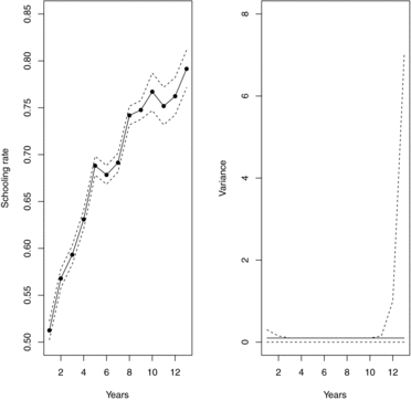
Note that the variance upper bound, close to year 12, is larger compared with other years. This feature agrees with the prediction interval of the mean, that is wider at year 12. However, when comparing the limits of the prediction interval for the model with random effects (Fig. 2) with the limits of the former model (Fig. 1), we found that the variance of the model with random effects is actually much smaller, and therefore it has a better model fit.

Figure 2 Normal nonlinear model with a random effect. (a) Prediction: fitted posterior mean (solid line) and 95% prediction interval (dotted lines). (b) Posterior variance with uncertainty limits.