
Abstract
The case that the factor model does not account for all the covariances of the observed variables is considered. It is shown that principal components representing covariances not accounted for by the factor model can have a nonzero correlation with the common factors of the factor model. The substantial correlations of components representing variance not accounted for by the factor model with common factors are demonstrated in a simulation study comprising model error. Based on these results, a new version of Harman's factor score predictor minimizing the correlation with residual components is proposed.
1. Introduction
The factor model has been developed primarily in psychology and has meanwhile been applied to a broad variety of data in many fields, even outside of psychology. A merit of the model is that latent variables can be constructed that may explain the covariances between observed variables. The model has been described in several books (e.g., Gorsuch, Citation1983; Harman, Citation1976; Harris, Citation2001; Mulaik, Citation2010; Tabachnick and Fidell, Citation2007) and several software packages are available for the calculation of the model. Nevertheless, it might not be regarded as a realistic assumption that the factor model fits perfectly to the data (MacCallum, Citation2003; MacCallum and Tucker, Citation1991; MacCallum et al., Citation2007). MacCallum and Tucker (Citation1991) called the misfit of the factor model in the population model error and they also describe sources of sampling error for the factor model. Both model error and sampling error might have the effect that the factor model does not account completely for the covariance of observed variables.
With respect to the model error in the population it is conceivable to extract just some more factors in order to minimize model error, although MacCallum and Tucker (Citation1991) warned that this will result in loss of parsimony (p. 504). However, Tucker et al. (Citation1969) constructed a model error that is based on a number of minor factors that is larger than the number of observed variables. In these situations, it would be impossible to eliminate model error completely by means of the extraction of some additional factors. Moreover, sampling error will also lead to nonzero residual covariances, even when the residual covariances are zero in the population. In these situations, it will probably not be reasonable to extract factors representing sampling error in order to get zero residual covariances in the sample. It is therefore concluded that nonzero residual covariances will sometimes be inevitable.
Whereas MacCallum (Citation2003) as well as MacCallum and Tucker (Citation1991) were concerned with the consequences of model error and sampling error for the model description and for the estimation of model parameters, the present paper investigates the correlation of the variance not accounted for by the factor model with the common factors. Beauducel (Citation2013) found that the correlation between the variance not accounted for by the principal component model and the common factors is not necessarily zero. This means that variance that is regarded as irrelevant according to principal component analysis can be relevant for the common factors. In contrast, the present paper investigates the correlation of the variance not accounted for by the factor model with the common factors. Since this variance is not part of the factor model, one would expect this variance to be uncorrelated with the common factors.
2. Definitions
The defining equation of the common factor model is
(1) where X is the random vector of observations of order p, f is the random vector of factor scores of order q, e is the unobservable random error vector or error factor of order p, and Λ is the factor pattern matrix of order p by q. The common factor scores f, and the error factors e are assumed to have an expectation zero (ϵ(X) = 0, ϵ(f) = 0, ϵ(e) = 0). The expected variance of the factor scores is one, the expected covariance between the common factors and the error factors is assumed to be zero (Cov(f, e) = ϵ(fe′) = 0). The expected covariance matrix of observed variables Σ can be decomposed into
(2) where Φ represents the q by q factor correlation matrix and
is a p by p diagonal matrix representing the expected covariance of the error factors e (Cov(e, e) = ϵ(ee′) =
). Moreover, postmultiplication of Eq. (1) with e′ shows that the expected covariance of the error factors with the observed variables is Cov(e, X) = ϵ(eX′) =
, because ϵ(fe′) = 0. It is assumed that the diagonal of
contains only positive values so that
is nonsingular.
According to MacCallum and Tucker (Citation1991), we consider that the factor model in the population does not account for the covariance of the observed variables completely. They argue that there could be large numbers of minor common factors or nonlinear relations between factors and observed variables that cannot be part of the model as it is represented in Eqs. (1) and (2). It is therefore necessary to take into account what MacCallum and Tucker (Citation1991) call model error. This yields
(3) with Ω representing the expectation of the residual covariances in the population.
When the factor model is estimated from S, the sample covariance matrix of observed variables, this yields
(4) where the subscript denotes that the parameters are estimates of the corresponding population parameters. The difference between Eqs. (3) and (4) implies that nonzero residual covariances in the sample could occur because of sampling error (
≠ 0) even when there are no residual covariances in the population (
= 0). Thus, there are two possible reasons for residual covariances: Sampling error and model error. However, in practical applications of the factor model the residual covariance term is usually omitted, so that
(5) and
(6) and ϵ(eses′) =
and ϵ(fses′) = 0 is assumed, which might be wrong to some more or less acceptable degree. If the model fit in the sample is perfect the residual covariances are zero (Ωs = 0) and if the model fit is not perfect in the sample, the residual covariances are not zero. It is considered in the following that the model fit is not perfect and that the imperfect model fit might be due to sampling error and/or to model error.
3. Results
Since the factor model as defined in Eq. (4) accounts for all diagonal elements in S, there are only nondiagonal elements in . The remaining definitions of the factor model are not altered by Eq. (4), only the nonzero nondiagonal elements in
are taken into account. Let Ωs = KVK′ with KK′ = K′K = I be the eigen-decomposition of
, where V is diagonal with the eigenvalues in decreasing order. Since the main-diagonal of
contains only zero values, the trace of V will be zero. Therefore, even when some nondiagonal elements of
are not zero, only the first eigenvalues of
will be positive and some negative eigenvalues will also occur. In the following, only the eigenvectors corresponding to positive eigenvalues are considered. The matrix K* contains only eigenvectors corresponding to positive eigenvalues and V* contains only positive eigenvalues (in descending order), so that Ns = K*V*1/2. Ns is called the loading matrix of the corresponding principal components.
is the matrix of sample estimates of residual covariances reproduced from the principal components with positive eigenvalues, with
(7) Accordingly, the corresponding residuals of the observed variables can be decomposed into principal components us, which yields
(8) with us being orthogonal components (usus′ = I). It follows from Eq. (8) and from Eqs. (5) and (6) that
(9) and that
(10) Theorem 3.1 states that when the residual covariances are not zero (NsNs′≠ 0) and when the expected correlation between the error vector es and the residual components us is zero, a nonzero expected correlation of the common factors fs with us occurs.
Theorem 3.1.
ϵ(fsus′) ≠ 0 if ϵ(esus′) = 0 and NsNs′≠ 0.
Proof.
It follows from Eqs. (7)–(9) that
(11) For ϵ(esus′) = 0, Eq. (11) can be transformed into
(12) Eq. (12) is true iff ϵ(Λsfsus′) = −0.5 Ns. This completes the proof. □
Theorem 3.2 specifies the condition for the expected zero correlation of the common factors fs with the residual components us when the residual covariances are not zero.
Theorem 3.2.
ϵ(fsus′) = 0 iff ϵ(esus′) = −0.5 Ns when NsNs′≠ 0.
Proof.
For ϵ(fsus′) = 0, Eq. (11) can be transformed into
(13)
Eq. (10) is true iff ϵ(esus′) = −0.5 Ns. This completes the proof. □
Theorem 3.3 specifies that the expected correlation of the variance accounted for by the factor model (sfs + es) with the residual components us is not zero when the residual covariances are not zero.
Theorem 3.3.
ϵ((Λsfs + es)us′) ≠ 0 when NsNs′≠ 0.
Proof.
Eq. (11) can be transformed into
(14) Eq. (11) is true iff ϵ((Λsfs + es)us′) = −0.5 Ns. This completes the proof. □
The meaning of Theorem 3.3 is that the components us, representing variance not accounted for by the factor model, have a nonzero correlation with the variance accounted for by the factor model.
Transformation of Eq. (8) reveals that the components us can be calculated as
(15) Both fs and es are usually unknown in empirical analyses due to factor score indeterminacy (Guttman, Citation1955; Mulaik, Citation2010) so that Eq. (15) implies that indeterminacy also holds for us. Thus, in a typical situation of an applied researcher, the correlation of the components representing the variance not accounted for by the factor model with the common factors remains unknown. Nevertheless, a modified version of the Harman factor score predictor minimizing the correlation of the factor score predictor with the components representing the residual variance is proposed for practical application. The Harman factor score predictor (Harman, Citation1976) is
(16) so that
(17) It follows from Eq. (17) that a modified Harman factor score predictor fsM based on a modified loading matrix Λs* with Ns′Λs* = 0 yields ϵ(usfsM′) = 0. The modified loading matrix with Ns′Λs* = 0 can be calculated as
(18) because premultiplication of Eq. (18) with Ns′ yields 0. Thus, for practical applications
(19) allows for a factor score predictor that minimizes the correlation with the components representing the variance not explained by the common factor model. If the residual correlations are not completely represented by Ωs* the correlation of fsM with us will not necessarily be zero, but it will be smaller than the correlation of the factors with us. It should also be noted that Ωs* is estimated in the sample as the difference between the empirical covariance matrix and the reproduced covariance matrix, i.e., Ωs* = S – (ΛsΦs Λs ′ + Ψs2). The precision of this estimate depends on the precision of the estimates of the parameters of the factor model, so that different estimation methods of the factor model (MacCallum et al., Citation2007) might lead to different results.
3.1 Simulation Study
The magnitude ofthe correlations between the common factors and the components representing the residuals cannot be investigated within empirical studies, because the population common factor scores and the population error factor scores are unknown. However, in simulation studies population common factor scores and population error factor scores can be fixed a priori so that their correlation with the components representing residuals can be investigated. Therefore, a simulation study was conducted in order to investigate the size of the correlations between the common factors and components representing the variance that is not accounted for by the factor model.
Table 1 Three-factor population models based on salient loadings of.40
Table 2 Means and standard deviations (in brackets) of eigenvalues of the first principal component calculated from the residual correlations
All components with positive eigenvalues representing the variance not accounted for by the factor model were considered in this simulation. The simulation study splits up into two parts: The first part starts from population models that hold in the population, so that the residual components derived from factor analyses of the corresponding samples only represent variance that is due to sampling error. In the first part, the population correlation matrices can directly be computed from the factor loadings and the uniquenesses. The second part of the simulation study starts from the same parameters of the population models, but the population models are not “true” in the population. In this part of the simulation study, the population correlation matrices are generated from the loadings of the major factors as well as from the loadings of 100 “minor factors” and from the corresponding uniquenesses. Minor factors have very small nonzero population loadings and represent the “many minor influences” (Tucker et al., Citation1969), which affect the values of the observed scores in the real world. The loading matrices of the minor factors were generated according to the procedure reported in MacCallum and Tucker (Citation1991). The loadings of the minor factors were therefore generated from z-standardized normally distributed random numbers, where the relative contribution of factors was successively reduced by the factor.8, and the amount of variance explained by the minor factors was set to 10% of the observed total variance. Accordingly, the first four minor factors explained 2.0%, 1.6%, 1.3%, and 1% of the variance. All loadings of minor factors were between –1 and +1. Since minor factors were introduced into the population data, a factor model that is only based on the population parameters of the major factors contains necessarily model error. As an example, a population correlation matrix of observed variables for a three-factor model based on moderate salient loadings (.6) and model error is given in the Appendix (Table A1). The residual components derived from factor analyses of the corresponding samples contain model error and sampling error.
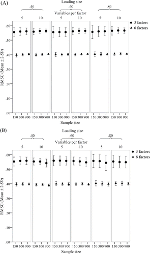
The conditions of both simulation studies (without andwith model error) were the number of cases in the sample (150, 300, 900 cases), the size of the salient loadings (.40,.60,.80), the number of factors (3, 6 factors), and the number of variables with salient loadings per factor (5, 10). For each of the 36 conditions (3 numbers of cases × 3 loading sizes × 2 numbers of factors × 2 numbers of salient loadings) 1,000 factor analyses were performed with SPSS 20. As an example, the population three-factor model for salient loadings of.40 is presented in . Since orthogonal population models were investigated, Varimax-rotation (Kaiser, Citation1958) was performed for the 36,000 maximum likelihood factor analyses based on the random samples drawn from the population. The factor analyses were based on the correlations of the observed variables.
Table 3 ANOVA results for the root mean squared correlation (RMSC) of the components representing the residual correlations from factor analysis with the common factors in simulation study
The mean eigenvalues of the first components representing the correlations not accounted for by the factor model were larger for smaller sample sizes and for smaller salient loading sizes (see ). This was to be expected, since no model error was present in this part of the simulation study so that the first component should only represent residual correlations that are due to sampling error.
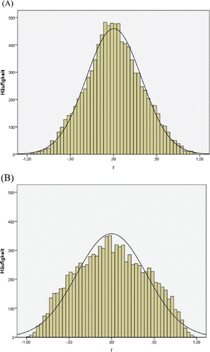
The distributions of the correlations of the first component representing the residual correlations of factor analysis with the first common factor are presented in . Although the distributions are quite symmetric, the kurtosis of the distribution of correlations was a bit smaller when based on the six-factor solutions ((A)) than the kurtosis of the distribution of correlations for the three-factor solutions ((B)). More importantly, the whole range of positive and negative correlations occurred, with 17.1% of the correlations with an absolute size greater than.80 for the three-factor solutions and 2.9% of the correlations with an absolute size greater than.80 for the six-factor solutions.
In order to provide a more complete description of the effects of the conditions of the simulation study, the root mean squared correlation (RMSC) of the residual components with positive eigenvalues with the common factors was computed. The ANOVA results are reported in . Of course, due to the large sample size of the simulation study, all condition main effects and all interactions were significant in ANOVA at the.001 level so that the interpretation of the results should be based on effects sizes. The effect size of the number of factors was extremely large whereas the effect size of the remaining conditions was extremely small. This result can also be depicted from Fig. 2(A): The RMSC was about.55 for the three-factor solutions and was about.40 for the six-factor solutions. Thus, the RMSC decreases with the number of factors, but it does not decrease substantially with sample size and with the size of the salient loadings. Interestingly, the results of the simulation study based on the combined effects of model error and sampling error were virtually the same as the results based on the simulation study that only containssampling error (Fig. 2(B)). Thus, both sampling error and model error induced residual components that correlate substantially with the common factors.
The Harman factor score predictor and the corrected Harman factor score predictor were also computed for the samples and correlated with the residual components with positive eigenvalues. It should be noted that the RMSC of the factor score predictors with the residual components were smaller than for the factors themselves (see ). Again, the RMSC were smaller for the six-factor models than for the three-factor models. Moreover, the RMSC with the residual components were substantially smaller for the corrected Harman factor score predictor than for the conventional Harman factor score predictor, indicating that the correction has the intended effect (see Table 4).
Table 4 Root mean square residual correlations (RMSC) of the Harman factor score predictor and the corrected Harman factor score predictor with the residual components
4. Discussion
The correlation of components representing the variance not accounted for by the factor model with the common factors was investigated. Since this unexplained variance is by definition not part of the factor model, one would expect components representing this variance to be uncorrelated with the common factors. However, it was shown algebraically and by means of a simulation study with and without population model error (MacCallum et al., Citation2007) that the common factors can have in fact a nonzero correlation with components representing the variance not accounted for by the factor model. Moreover, the sum of the common factors and the error factors representing the total variance that is accounted for by the factor model was shown to have a nonzero correlation with the variance not accounted for by the factor model. According to Theorem 3.3, the common factors are uncorrelated with the components representing unexplained variance only under a condition implying that the error factors have a nonzero correlation with these components. The simulation study revealed that the root mean squared correlation of the components representing unexplained variance with the common factors was about.55 for the three-factor solutions and about.40 for the six-factor solutions. It should be concluded that these correlations cannot be regarded as being virtually zero in general. Since factor analysis will nearly always be performed on sample data and since this would always lead to some covariances that are not accounted for by the factor model (MacCallum, Citation2003; MacCallum and Tucker, Citation1991), the results presented here will be relevant for most applications of factor analysis. Moreover, the simulation study also included model error based on a number of minor factors that was larger than the number of observed variables, so that the residual variance cannot be eliminated completely by extracting some more factors.
A modified version of Harman's factor score predictor that minimizes the correlation with the components representing the unexplained variance is proposed. It is shown in the simulation study that this factor score predictor has lower correlations with the residual components than the conventional version of Harman's factor score predictor. Therefore, the modified version of Harman's factor score predictor can be recommended for practical applications.
References
- Beauducel, A. (2013). A note on unwanted variance in exploratory factor models. Communications in Statistics – Theory and Methods 42:561–565.
- Gorsuch, R.L. (1983). Factor Analysis. 2nd ed. Hillsdale, NJ: Erlbaum.
- Guttman, L. (1955). The determinacy of factor score matrices with applications for five other problems of common factor theory. British Journal of Statistical Psychology 8:65–82.
- Harman, H.H. (1976). Modern Factor Analysis. 3rd ed. Chicago: The University of Chicago Press.
- Harris, R.J. (2001). A Primer of Multivariate Statistics. 3rd ed. Hillsdale, NJ: Erlbaum.
- Kaiser, H.F. (1958). The varimax criterion for analytic rotation in factor analysis. Psychometrika 23:187–200.
- MacCallum, R.C. (2003). Working with imperfect models. Multivariate Behavioral Research 38:113–139.
- MacCallum, R.C., Browne, M.W., Cai, L. (2007). Factor analysis models as approximations. In: Cudeck, R.,C.MacCallum, R.C., eds. Factor Analysis at 100: Historical Developments and Future Directions, Mahwah, NJ: Lawrence Erlbaum, pp. 153–175.
- MacCallum, R.C., Tucker, L.R. (1991). Representing sources of error in the common-factor model: Implications for theory and practice. Psychological Bulletin 109:502–511.
- Mulaik, S.A. (2010). Foundations of Factor Analysis. 2nd ed. New York: CRC Press.
- Tabachnick, B.G.,S.Fidell, L.S. (2007). Using Multivariate Statistics. 5th ed. Boston, MA: Pearson Education.
- Tucker, L.R., Koopman, R.F., Linn, R.L. (1969). Evaluation of factor analytic research procedures by means of simulated correlation matrices. Psychometrika 34:421–459.
Appendix