A wavelet approach for profile monitoring of Poisson distribution with application

Abstract

Profile monitoring is defined as the act of utilizing regression and quality control techniques to monitor the functional relationship between a response variable and one or more regressors. Most of the previous studies focused either on parametric modeling of profiles or assumed the response variable followed a normal distribution, but that is an unrealistic scenario in most cases. In this study, a Haar wavelet approach is applied for profile monitoring of Poisson data. We showed via simulation that, Haar wavelet can outperform parametric models when there is a sudden jump in the profile and concluded with a case study.

Keywords:

• Nonparametric Regression
• Poisson
• Profile Monitoring
• Haar Wavelet
• Quality Control

1. Introduction

Profile monitoring is a relatively new technique in statistical process control (SPC). Kang and Albin (2000) defined a profile as the functional relationship between a response variable and one or more regressors. Depending on the type of this relationship, linear and nonlinear profiles can be utilized. Profile monitoring is defined as the act of using statistical methods to monitor the changes in a process or product.

One common assumption in the literature is that the relationship between the response variable and the explanatory variables can be expressed by a certain function. However, in some real world problems it is hard to find a certain parametric model that can describe the aforementioned relationship. This issue has been addressed by several authors such as Härdle (1992), Fan and Gijbels (1996), Green and Silverman (1994), Kim, Mahmoud, and Woodall (2003), Mahmoud and Woodall (2004), and Mahmoud et al. (2007). In their works, they provided data examples which could not be modeled via parametric models and utilized nonparametric regression techniques to monitor those profiles. Works done by Reis and Saraiva (2006), Jeong, Lu, and Wang (2006) and Chicken, Pignatiello, and Simpson (2009) presented other nonparametric regression profile monitoring techniques.

A popular tool used to fit the nonparametric regression models are smoothers which depending on the type of data can be applied. For handling sparse data, smoothing splines are recommended while polynomial smoothers are preferred for handling dense deigns. Popular smoothers through out the literature are local polynomial smoothers which were used by Fan and Gijbels (1996), regression splines, smoothing splines Wahba (1990), Green and Silverman (1994), Mays and Birch (2002), Mays et al. (2001), Mays et al. (2000), Wang (2011) and penalized splines Ruppert et al. (2003).

Wavelets can be used as a nonparametric regression to model profiles with sudden changes. Wavelet has proved to be a popular tool by researchers when the profile data cannot be described by simple models. It is usually recommended when the shape of the profile is too complicated to be modeled by a linear or nonlinear model (Woodall (2007)). Nonparametric wavelet models have been used in the works of Reis and Saraiva (2006), Jeong, Lu, and Wang (2006), Zou, Wang, and Tsung (2007), and Chicken, Pignatiello, and Simpson (2009) and control charts were made based on a subset of wavelet estimates. In the work by Reis and Saraiva (2006), a multi scale framework based on wavelets was introduced for the monitoring of of both roughness and waviness of paper surface. Jeong, Lu, and Wang (2006) presented a SPC procedure that adaptively determines which wavelet coefficients to monitor and showed that their method performed effectively in detecting many types of process changes. Chicken, Pignatiello, and Simpson (2009) suggested a method based on semi-parametric wavelets for monitoring the changes in sequences of nonlinear profiles. Based on a likelihood ratio test which incorporated a change point model, their method used the spatial adaptivity characteristics of wavelets to appropriately detect profile changes. Chang and Yadama (2010) applied a Discrete wavelet transformation (DWT) to separate variation or noise from profile contours and also by using B-splines which generate critical points they defined the shape of profiles. The novelty of their work was that, it enabled users to divide a profile into multiple segments and monitor them simultaneously. Nikoo and Noorossana (2013) used approximate wavelet coefficients for profile monitoring of Vertical Density Profiles and introduced an ANOVA based method to find the perfect resolution level for wavelet estimates.

Normality assumption of the response variable is a very common assumption among studies done by researchers. Although, this assumption can be correct in some cases, there are many cases that the variable of interest is not continuous but is a count or frequency, such as the number of defects in a manufacturing process or the number of customers who visited a webpage (Poisson distribution). Ignoring other distributions can cause misleading results Noorossana et al. (2008). Several authors have addressed this in their studies Nelder and Jacob Baker (1972), McCullagh and Nelder (1989), McCulloch and Searle (2001), Schabenberger and Pierce (2001), Hastie and Tibshirani (1990), Ruppert et al. (2003), Yeh et al. (2009) and Amiri et al. (2011). Although, literature on profile monitoring for non-normal responses, especially binary ones, is rich, few works have been done on profile monitoring for Poisson responses. Amiri et al. (2011) examined two of the five proposed T² methods by Yeh et al. (2009) and proved that when the T² is derived from sample average and intra-profile, pooling it can perform better in detecting two type of shifts: step and drifts. Sharafi et al. (2013) introduced an Maximum Likelihood Estimator (MLE) estimator to detect the the time of a step change in profile monitoring of Poisson data in phase II and showed through simulation that the estimator was effective in detecting step shifts. Asgari et al. (2014) proposed a new method to monitor a two stage process where the second stage had Poisson variable. They combined the logarithm and the square root link functions and, instead of using deviance residuals which was used in the r method of Skinner et al. (2003), a standardized residual (SR) statistic was used.

Amiri et al. (2015) developed, modified, and compared three methods: one was based on T², the second was based on likelihood ratio test (LRT), and the last was an F method. Performance of the three methods were compared when applied to Poisson response data. Their results showed that, for detecting two types of shifts (step and drift); the model based on likelihood ratio test (LRT) outperformed the others, and the method based on T² had the poorest performance. In terms of detecting outliers, F method proved to be the best and LRT had the poorest performance compared to the others. In the end, they applied these three methods to a real-world profile monitoring with profiles describing the relationship between the size and number of agglomerates emitted from a volcano in consecutive days and demonstrated that they were successful in distinguishing the out of control situations.

This study focuses on the phase I analysis, where we are interested in understanding the variation and stability of the process and removing any outlying sample via analyzing a historical data set. The purpose is to setup the control limits for phase II analysis. In this paper, addressing two novel issues; firstly profile monitoring for the Generalized exponential distribution where the Poisson is considered as the distribution of the response variable instead of the common normality assumption. Second, profiles are not always easily modeled by parametric approaches and there is a need for a data driven approach (wavelet) that would capture the shape of the profiles, especially those with abrupt changes. The performance of parametric and wavelet approach in profile monitoring of Poisson data with sudden jump via comprehensive simulation studies. In the end, a real case scenario utilize to compare the performance of the proposed approach with some state-of-the-arts. In the rest of the paper, Sec. 2 describes the parametric, wavelet methods and their applications in profile monitoring of Poisson data in detail. Section 3 presents the simulation study and provides a comparison on the performance of these models in different situations. Section 4, concludes the application of proposed models by showing their performance in a real- world case study.

2. Methodology

In this section, we explain the parametric and wavelet models with their applications in profile monitoring of Poisson data.

2.1. Parametric approach

Parametric profile monitoring assumes that, the relationship between the response variable and the covariates can be represented by a certain linear or nonlinear function. The basic idea of parametric profile monitoring involves two steps. First, an appropriate statistical model is used to characterize the profile. The choice of that model depends on the characteristics of the profile data. Second, regression parameters’ estimates are monitored by using multivariate control charts such as Hotelling’s T² or Exponential Weighted Moving Average (EWMA) Noorossana et al. (2008).

In simplest case, observations in the ith profile can be modeled via a simple regression model as follows: (1) $$y_{ij}={\beta }_{i0}+{\beta }_{i,1}{X}_{i,j}+{ϵ}_{i,j},i=1,2,\dots ,m,j=1,2,\dots ,n_i$$(1)

Where y_ij is the jth observation in the ith profile, $X_{i,j}$ is the jth value of the explanatory variable for ith profile and ${ϵ}_{i,j}$ is the random variable of jth observation in ith profile.

Suppose there are n independent observations in a profile where each of them follows a Poisson distribution with a mass probability function as follows: (2) $$f\left(Y_i\right)=\frac{e^{-{\lambda }_i}{\lambda }_i{}^{Y_i}}{Y_i!},\hspace{1em}i=1,2,\mathrm{\dots \dots },n,Y_i>0$$(2)

Hence, $E(Y_i)={\lambda }_i$ and $Var(Y_i)={\lambda }_i$. In addition, let ${\eta }_i={\beta }_0+{\beta }_1{x}_i$. With Log link transformation, λ_i can be described as a function of η_i. Therefore, (3) $$g\left({\lambda }_i\right)=\hspace{0.17em}\text{log}\hspace{0.17em}\left({\lambda }_i\right)={\beta }_0+{\beta }_1{x}_i$$(3) where β₀ and β₁ are regression parameters. Based on Eq. (3)(3) $$g\left({\lambda }_i\right)=\hspace{0.17em}\text{log}\hspace{0.17em}\left({\lambda }_i\right)={\beta }_0+{\beta }_1{x}_i$$(3) the following equation can be obtained: (4) $${\lambda }_i=\hspace{0.17em}\text{exp}\hspace{0.17em}\left({\eta }_i\right),i=1,2,\mathrm{\dots \dots },n$$(4)

Given that the observations are independent from each other, the joint likelihood function of $Y_1,Y_2,\dots ,Y_n$ is as follows: (5) $$L({\lambda }_i,y_i)=\prod _{i=1}^n{e}^{-{\lambda }_i}\frac{{\left({\lambda }_i\right)}^{Y_i}}{Y_i!}=e^{-\sum _{i=1}^n\left({\lambda }_i\right)}\frac{{\prod }_{i=1}^n{\left({\lambda }_i\right)}^{Y_i}}{{\prod }_{i=1}^n{Y}_i!}$$(5)

Taking logarithm of both sides of Eq. (5)(5) $$L({\lambda }_i,y_i)=\prod _{i=1}^n{e}^{-{\lambda }_i}\frac{{\left({\lambda }_i\right)}^{Y_i}}{Y_i!}=e^{-\sum _{i=1}^n\left({\lambda }_i\right)}\frac{{\prod }_{i=1}^n{\left({\lambda }_i\right)}^{Y_i}}{{\prod }_{i=1}^n{Y}_i!}$$(5) and using Eq. (4)(4) $${\lambda }_i=\hspace{0.17em}\text{exp}\hspace{0.17em}\left({\eta }_i\right),i=1,2,\mathrm{\dots \dots },n$$(4) the following equation can be obtained: (6) $$\text{log}\left[L\right({\lambda }_i,y_i\left)\right]=\sum _{i=1}^n{Y}_i\hspace{0.17em}\text{log}\hspace{0.17em}(\hspace{0.17em}\text{exp}\hspace{0.17em}({\eta }_i\left)\right)-\sum _{i=1}^n\hspace{0.17em}\text{exp}\hspace{0.17em}\left({\eta }_i\right)-\sum _{i=1}^{n}log(Y_i!)$$(6)

Taking the derivative of Eq. (6)(6) $$\text{log}\left[L\right({\lambda }_i,y_i\left)\right]=\sum _{i=1}^n{Y}_i\hspace{0.17em}\text{log}\hspace{0.17em}(\hspace{0.17em}\text{exp}\hspace{0.17em}({\eta }_i\left)\right)-\sum _{i=1}^n\hspace{0.17em}\text{exp}\hspace{0.17em}\left({\eta }_i\right)-\sum _{i=1}^{n}log(Y_i!)$$(6) with respect to β the following equation will be obtained where ${\mu }_i={\lambda }_i$ and $X_i=[1x_i]$: (7) $$\frac{\partial \hspace{0.17em}\text{log}\left[L\right({\lambda }_i,y_i\left)\right]}{\partial \beta }=\sum _{i=1}^n{X}_i{Y}_i-\sum _{i=1}^n{X}_i{\mu }_i=\sum _{i=1}^n(Y_i-{\mu }_i)X_i$$(7)

Based on (7), the MLE estimator of β can be found by solving the following equation where $0={(0,\dots ,0)}^T$ and $\mu =({\mu }_1,\mathrm{\dots .},{\mu }_n)$: (8) $$X^T(y-\mu )=0$$(8)

Using iterative weighted least squares (IRWLS) the MLE estimators of $\beta \prime s$ can be calculated following the algorithm below:

Step (1): Let ${\widehat{\beta }}^{[0]}$ be the initial estimate of β which can be obtained using ordinary least squares (OLS), set R = 0. Step (2): Using ${\widehat{\beta }}^{(R)}$ estimate, compute ${\eta }_i{}^{(R)}$ and ${\lambda }_i{}^{(R)}$ using Eqs. (3)(3) $$g\left({\lambda }_i\right)=\hspace{0.17em}\text{log}\hspace{0.17em}\left({\lambda }_i\right)={\beta }_0+{\beta }_1{x}_i$$(3) and (4)(4) $${\lambda }_i=\hspace{0.17em}\text{exp}\hspace{0.17em}\left({\eta }_i\right),i=1,2,\mathrm{\dots \dots },n$$(4) Step (3): Define matrix W using Eq. (9)(9) $$W^{\left(R\right)}=\mathit{\text{diag}}\left({\lambda }_i{}^{\left(R\right)}\right)$$(9) (9) $$W^{\left(R\right)}=\mathit{\text{diag}}\left({\lambda }_i{}^{\left(R\right)}\right)$$(9)

where W is an n × n matrix

Step (4): Compute adjusted dependent variate q_i where (10) $$q_i^{\left(R\right)}={\eta }_i^{\left(R\right)}+{\left(W^{\left(R\right)}\right)}^{-1}(y_i-{\mu }_i)$$(10) Step (5): Update β estimates using Eq. (10)(10) $$q_i^{\left(R\right)}={\eta }_i^{\left(R\right)}+{\left(W^{\left(R\right)}\right)}^{-1}(y_i-{\mu }_i)$$(10) (11) $${\beta }_i^{\left(\right(R)+1)}={\left(X^T{W}^{\left(R\right)}X\right)}^{-1}{X}^T{W}^{\left(R\right)}{q}_i^{\left(R\right)}$$(11)

Set $R=R+1$

Step (6): Repeat steps 2 through 5 for k times till algorithm converges. We say the algorithm converges when $\frac{\left|\right|{\widehat{\beta }}^{[K]}-{\widehat{\beta }}^{[K-1]}\left|\right|}{\left|\right|{\widehat{\beta }}^{[K-1]}\left|\right|}\le \alpha$. $\left|\right|x\left|\right|$ is defined as the Euclidean norm of a vector x and we chose α to be a sufficient small constant (e.g, $\alpha ={10}^{-5}$). $\widehat{\beta }={\widehat{\beta }}^{[K]}$ would then be the optimum estimator of β.

Yeh et al. (2009) proposed 5 different control charts, the below method below is one of the top ones among them. Using the equation below, one can compute the T² values for each profile. (12) $$T^2{}_{P,i}={(\widehat{{\beta }_i}-\overline{\beta })}^T{S}_D{}^{-1}(\widehat{{\beta }_i}-\overline{\beta }),i=1,2,\mathrm{\dots \dots },m$$(12) where m is the number of profile, $\widehat{\beta }$ is the regression coefficient estimate for each profile and $\overline{\beta }$ and S_D can be calculated with the following equations: (13) $$\overline{\beta }=\frac{1}{m}\sum _{i=1}^m\widehat{{\beta }_i}$$(13) (14) $$S_D=\frac{1}{2(m-1)}\sum _{i=1}^{m-1}({\widehat{\beta }}_{i+1}-{\widehat{\beta }}_i){({\widehat{\beta }}_{i+1}-{\widehat{\beta }}_i)}^T$$(14)

Successive differences, S_D, which is an estimator proposed by Williams et al. (2006) is very practical for detecting the step shift in profiles.

It is desired from the T² control chart to give a signal whenever the values of $T_{P,i}^2$ exceeds the UCL, Upper Control Limit, which is defined as an approximated chi-square distribution with a degree of freedom equal to number of parameters used to compute the T². A signal is given whenever $T^2{}_{P,i}\ge {\chi }^2{}_{d{f}_P,\alpha }$ where df_P represents degrees of freedom and α represents the significance level. In the case of parametric profile monitoring, the df_P equals to two given that simple regression is being used and α is assumed to be 0.05.

2.2. Wavelet approach

There are various wavelet families available for nonparametric regression. In this work, we are using Haar wavelet. The process of approximating a function via wavelets is quite straightforward. First, a wavelet from family of wavelets is chosen to transform the function into wavelet components. Second, the wavelet components are thresholded using different policies and methods. Third, threshold wavelet components are reconstructed via pyramid algorithm. Every wavelet basis is made from a mother wavelet and a scaling function also known as the father wavelet. When approximating functions via Haar wavelet, there are certain assumptions that need to be met. First, the number of observations should be a power of two. Second, the function’s range should be defined on [0,1) interval. A function can be estimated with a Haar wavelet that is constructed from a mother and a father wavelet: (15) $$y\left(t\right)=\sum _{k=0}^{2^{j_0-1}}{c}_{j_{0}k}{\varphi }_{j_{0}k}\left(t\right)+\sum _{j=j_0}^J\sum _{k=0}^{2^{j-1}}{d}_{jk}{\psi }_{jk}\left(t\right)$$(15)

In Eq. (15)(15) $$y\left(t\right)=\sum _{k=0}^{2^{j_0-1}}{c}_{j_{0}k}{\varphi }_{j_{0}k}\left(t\right)+\sum _{j=j_0}^J\sum _{k=0}^{2^{j-1}}{d}_{jk}{\psi }_{jk}\left(t\right)$$(15) , ${\varphi }_{j_{0}k}$ is the father wavelet which is made from the father wavelet basis defined as ${\varphi }_{j_{0}k}(x)=2^{j_0/2}\varphi (2^{j_0}x-k)$ and $c_{j_{0}k}$ are father/approximate wavelet coefficient. ψ_jk is the mother wavelet which is made from the mother wavelet base defined as ${\psi }_{j,k}(x)=2^{j/2}\psi (2^{j}x-k)$ and d_jk are detail/mother wavelet coefficients. As the value of J increases the quality of this approximation improves as well and J can range from 0 to $(p-1)$ where p is the ${\hspace{0.17em}\text{log}\hspace{0.17em}}_2(n)$ and n is the length of the data vector. For instance, if a data vector of size n = 128 is to be estimated by Haar wavelet, then $p=lo{g}_2(128)=7$ and the levels for J can range from J = 0 to J = 6. One of the advantages of using wavelets, as a nonparametric method is using thresholding as a way to clean noisy coefficients. Thresholding helps clean unimportant coefficients and results in describing a noisy function with relatively small number of wavelet coefficients. When a noisy function is transformed with a wavelet, some detail coefficients, $d_k^J$, capture the noise of the function and therefore removing them will not damage the overall fit of the function. In this work, we used a soft policy and compared the detail coefficients to λ, thresholding value, and removed those that met the conditions. The value of λ was calculated via universal thresholding. The soft policy and λ value are shown in Eq. (16)(16) $$\begin{array}{c}{\sigma }^S{}_{\lambda }\left({\widehat{d}}_{jk}\right)=\{\begin{array}{cc}0\hfill & \hspace{1em}\text{if}\hspace{1em}\left|{\widehat{d}}_{jk}\right|\le \lambda ,\hfill \\ {\widehat{d}}_{jk}-\lambda \hfill & \hspace{1em}\text{if}\hspace{1em}{\widehat{d}}_{jk}>\lambda ,\hfill \\ {\widehat{d}}_{jk}+\lambda \hfill & \hspace{1em}\text{if}\hspace{1em}{\widehat{d}}_{jk}<-\lambda .\hfill \end{array}\\ {\lambda }^U=\sqrt{2\hspace{0.17em}\text{log}\hspace{0.17em}n}\hspace{1em}\widehat{\sigma }\end{array}$$(16) : (16) $$\begin{array}{c}{\sigma }^S{}_{\lambda }\left({\widehat{d}}_{jk}\right)=\{\begin{array}{cc}0\hfill & \hspace{1em}\text{if}\hspace{1em}\left|{\widehat{d}}_{jk}\right|\le \lambda ,\hfill \\ {\widehat{d}}_{jk}-\lambda \hfill & \hspace{1em}\text{if}\hspace{1em}{\widehat{d}}_{jk}>\lambda ,\hfill \\ {\widehat{d}}_{jk}+\lambda \hfill & \hspace{1em}\text{if}\hspace{1em}{\widehat{d}}_{jk}<-\lambda .\hfill \end{array}\\ {\lambda }^U=\sqrt{2\hspace{0.17em}\text{log}\hspace{0.17em}n}\hspace{1em}\widehat{\sigma }\end{array}$$(16) where $\widehat{\sigma }=MAD(d_{n-1,i},i=1,\frac{N}{2})$ and $(n-1)$ is the highest level. MAD is median absolute deviation.

3. Simulation study

Since there is no study has been done on comparing the performance of parametric and wavelet approach on profile monitoring for a Poisson data, based on our best of knowledge, we decided to study this via a simulation. In this study, we compared the performances of these models when the underlying function is a step function which a sudden jump can be seen in it. In order to conduct a through simulation, a function was created in R which took into account the number of profiles, m = 3060, number of observations, $n=16,32$, size of the shift in location of the jumps for small, moderate and big changes, c (0, 0.125, 0.25, 0.5) and the last but not the least the magnitude of the jumps for small, moderate and big changes c(0, 0.125, 0.25, 0.5). We expected that this function would be very hard to estimate with parametric, because of its sudden jump, but relatively easy for Haar wavelet. The λ of the step function was 2 for the first half and 10 for the second half of observations for each profile. A shift of 0.5 in jump location and its magnitude is shown in Figure 1. Tables 1 and 2 support our assumptions. As shown in Table 1 the Haar estimate does a much better approximation than the parametric model. Of interest is the behavior of the models when the location of the jump is shifted to the right. The SIMSE of both models start to decrease as the jump starts shifting to the right since this allows the models to approximate a function that is mostly a straight line. As expected, the SIMSE and probability of signal of both models increased as the jump magnitude increased. Adding more observations to the profiles will result in a better fit for models and higher probability of signal, but adding more profiles will have no significant effect. The simulation studies show the superiority of the Haar wavelet approach to the parametric approach.

Figure 1. Mean for Step Data.

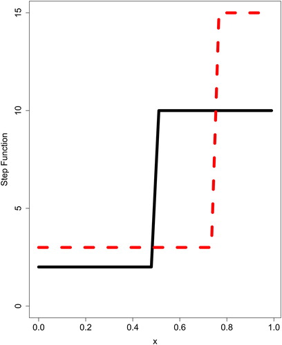
Table 1. m = 30 n = 16 for Step Function (Based on 1000 Replication Simulation Results).

				IMSE		P(Signal)
m	n	shift	height	Par	Wave	Par	Wave
30	16	0	0	6.21	3.00	0.051	0.055
30	16	0.125	0	5.77	2.86	0.073	0.089
30	16	0.25	0	5.34	2.73	0.123	0.197
30	16	0.5	0	4.93	2.47	0.291	0.607
30	16	0	0.125	7.01	3.19	0.080	0.080
30	16	0.125	0.125	6.46	3.04	0.060	0.079
30	16	0.25	0.125	5.93	2.89	0.074	0.156
30	16	0.5	0.125	5.40	2.61	0.197	0.581
30	16	0	0.25	7.91	3.40	0.164	0.151
30	16	0.125	0.25	7.23	3.26	0.098	0.109
30	16	0.25	0.25	6.57	3.06	0.071	0.164
30	16	0.5	0.25	5.95	2.72	0.123	0.577
30	16	0	0.5	9.97	3.83	0.393	0.354
30	16	0.125	0.5	9.00	3.67	0.278	0.264
30	16	0.25	0.5	8.05	3.40	0.179	0.250
30	16	0.5	0.5	7.19	3.00	0.065	0.588

Table 2. m = 30 n = 32 for Step Function (Based on 1000 Replication Simulation Results).

				IMSE		P(Signal)
m	n	shift	height	Par	Wave	Par	Wave
30	32	0	0	5.78	1.49	0.051	0.051
30	32	0.125	0	5.35	1.45	0.092	0.120
30	32	0.25	0	4.94	1.36	0.189	0.310
30	32	0.5	0	4.57	1.25	0.486	0.768
30	32	0	0.125	6.57	1.60	0.112	0.106
30	32	0.125	0.125	6.02	2.87	0.066	0.099
30	32	0.25	0.125	5.51	1.45	0.097	0.251
30	32	0.5	0.125	5.05	1.31	0.327	0.745
30	32	0	0.25	7.43	1.69	0.260	0.230
30	32	0.125	0.25	6.76	3.28	0.146	0.167
30	32	0.25	0.25	6.13	1.54	0.089	0.248
30	32	0.5	0.25	5.57	1.38	0.191	0.735
30	32	0	0.5	9.45	1.92	0.597	0.542
30	32	0.125	0.5	8.49	2.92	0.455	0.499
30	32	0.25	0.5	7.58	1.72	0.287	0.667
30	32	0.5	0.5	6.79	1.52	0.079	0.750

4. Case study

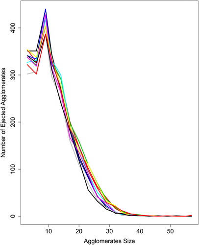
Now that we showed the superiority of the semi-parametric model over the parametric and nonparametric in our simulation study, it is time to assess these methods’ performance in a real-world profile monitoring situation. We decided to test the methods discussed in this study in profile monitoring on a volcano data set that was used in Amiri et al. (2015). The data was taken from a volcano in successive days. Profiles were defined as the relationship between the number of ejected agglomerates and agglomerate diameter. In this scenario, number of ejected agglomerates were a function of agglomerate diameter, which were counted by space images taken from the volcano each day. The first 10 profiles are shown in Figure 2.

Figure 2. Volcano Profiles.

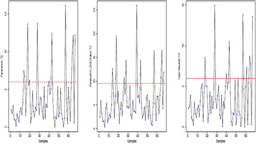
Looking at the Figure 3, the reader can see the obvious advantage of the $3^{rd}$ order parametric model over the $1^{st}$ order parametric and wavelet. The IMSE for $1^{st}$ order parametric, $3^{rd}$ order parametric and wavelet, are 4,227, 692, and 982 respectively and the T² for $1^{st}$ order parametric, $3^{rd}$ order parametric and wavelet are 0.16, 0.15, and 0.15 respectively. Figure 4 shows the T² control chart, where the T² values for profiles are shown and the red dashed line represents the upper control limit. The control chart for $1^{st}$ order parametric, $3^{rd}$ order parametric and wavelet give 11, 10, and 10 signals respectively which are quite close. However, the $3^{rd}$ order parametric model captures the shape of the profiles much better than the $1^{st}$ order parametric and wavelet and therefore can be more reliable in monitoring the changes in volcano profiles.

Figure 3. Real Data and Parametric Estimates.

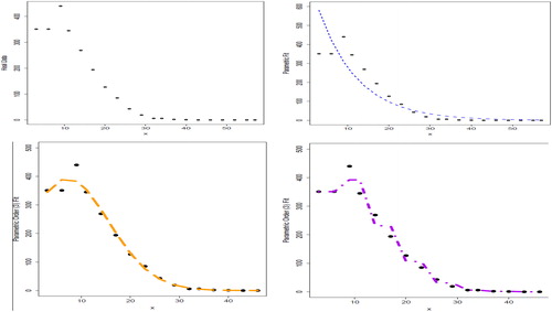
Figure 4. T² Control Charts for Parametric and Wavelet.

5. Conclusion and discussion

In this work, we compared first order and wavelet approaches for profile monitoring of Poisson data. These models were compared in a situation where there was a sudden jump in the profile. The simulation study showed that, the Haar wavelet would be a better option for fitting step changes in profiles for detecting changes than the misspecified parametric approach. In addition, the volcano case study showed that when the shape of the profiles are smooth and no sudden shift is happening, the proposed Haar wavelet is Superior than the parametric approach. The distribution of response was Poisson in this study, but other distribution of exponential family of distribution can be considered in future works.

References

- Amiri, A., M. Koosha, and A. Azhdari. 2011. Profile monitoring for Poisson responses. In Industrial Engineering and Engineering Management (IEEM), 2011 IEEE International Conference on, pp. 1481–1484. IEEE,
- Amiri, A., M. Koosha, A. Azhdari, and G. Wang. 2015. Phase I monitoring of generalized linear model-based regression profiles. Journal of Statistical Computation and Simulation 85 (14):2839–59. doi:10.1080/00949655.2014.942864.
- Asgari, A., A. Amiri, and S. T. A. Niaki. 2014. A new link function in GLM-based control charts to improve monitoring of two-stage processes with poisson response. The International Journal of Advanced Manufacturing Technology 72 (9):1243–56. doi:10.1007/s00170-014-5692-z.
- Chang, S. I., and S. Yadama. 2010. Statistical process control for monitoring non-linear profiles using wavelet filtering and B-spline approximation. International Journal of Production Research 48 (4):1049–68. doi:10.1080/00207540802454799.
- Chicken, E., J. J. Pignatiello, and J. R. Simpson. 2009. Statistical process monitoring of nonlinear profiles using wavelets. Journal of Quality Technology 41 (2):198–210. doi:10.1080/00224065.2009.11917773.
- Fan, J., and I. Gijbels. 1996. Local Polynomial Modelling and Its Applications. Boca Raton, FL: Chapman & Hall/CRC.
- Green, P. J., and B. W. Silverman. 1994. Nonparametric Regression and Generalized Linear Models: A Roughness Penalty Approach. London, New York: Chapman & Hall.
- Härdle, W. K. 1992. Applied Nonparametric Regression. Cambridge University Press.
- Hastie, T., and R. Tibshirani. 1990. Generalized additive models. Hoboken, NJ: John Wiley & Sons, Inc.
- Jeong, M., J. Lu, and N. Wang. 2006. Wavelet-based SPC procedure for complicated functional data. International Journal of Production Research 44:729–44.
- Kang, L., and S. L. Albin. 2000. On-line monitoring when the process yields a linear profile. Journal of Quality Technology 32 (4):418. doi:10.1080/00224065.2000.11980027.
- Kim, K., M. A. Mahmoud, and W. H. Woodall. 2003. On the monitoring of linear profiles. Journal of Quality Technology 35 (3):317. doi:10.1080/00224065.2003.11980225.
- Mahmoud, M. A., and W. H. Woodall. 2004. Phase I analysis of linear profiles with calibration applications. Technometrics 46 (4):380–91. doi:10.1198/004017004000000455.
- Mahmoud, M. A., P. A. Parker, W. H. Woodall, and D. M. Hawkins. 2007. A change point method for linear profile data. Quality and Reliability Engineering International 23 (2):247–68. doi:10.1002/qre.788.
- Mays, J. E., and J. B. Birch. 2002. Smoothing for small samples with model misspecification: nonparametric and semiparametric concerns. Journal of Applied Statistics 29 (7):1023–45. doi:10.1080/0266476022000006720.
- Mays, J. E., J. B. Birch, and B. Alden Starnes. 2001. Model robust regression: combining parametric, nonparametric, and semiparametric methods. Journal of Nonparametric Statistics 13 (2):245–77. doi:10.1080/10485250108832852.
- Mays, J. E., J. B. Birch, and R. L. Einsporn. 2000. An overview of model-robust regression. Journal of Statistical Computation and Simulation 66 (1):79–100. doi:10.1080/00949650008812013.
- McCullagh, P., and J. A. Nelder. 1989. Generalized linear models, no. 37 in monograph on statistics and applied probability. London: Springer.
- McCulloch, C. E., and S. R. Searle. 2001. Generalized linear mixed models (GLMMs). Generalized, Linear, and Mixed Models 220–46.
- Nelder, J. A., and R. Jacob Baker. 1972. Generalized linear models. Hoboken, NJ: John Wiley & Sons, Inc.
- Nikoo, M., and R. Noorossana. 2013. Phase II monitoring of nonlinear profile variance using wavelet. Quality and Reliability Engineering International 7:1081–89.
- Noorossana, R., A. Vaghefi, and M. Dorri. 2008. The effect of non-normality on performance of linear profile monitoring. In Industrial Engineering and Engineering Management, 2008. IEEM 2008. IEEE International Conference on, pp. 262–266. IEEE.
- Reis, M. S., and P. M. Saraiva. 2006. Multiscale statistical process control of paper surface profiles. Quality Technology & Quantitative Management 3:263–82.
- Ruppert, D., M. P. Wand, and R. J. Carroll. 2003. Semiparametric regression. Cambridge: Cambridge University Press.
- Schabenberger, O., and F. J. Pierce. 2001. Contemporary statistical models for the plant and soil sciences. Boca Raton, FL: CRC press.
- Sharafi, A., M. Aminnayeri, and A. Amiri. 2013. An MLE approach for estimating the time of step changes in poisson regression profiles. Scientia Iranica 20 (3):855–60.
- Skinner, K. R., D. C. Montgomery, and G. C. Runger. 2003. Process monitoring for multiple count data using generalized linear model-based control charts. International Journal of Production Research 41 (6):1167–80. doi:10.1080/00207540210163964.
- Yeh, A. B., L. Huwang, and Y.-M. Li. 2009. Profile monitoring for a binary response. IIE Transactions 41 (11):931–41. doi:10.1080/07408170902735400.
- Wahba, G. 1990. Spline Models for Observational Data. Philadelphia, Pa.: Society for Industrial and Applied Mathematics.
- Wang, Y. 2011. Smoothing Splines: Methods and Applications. Boca Raton, FL: CRC Press.
- Williams, J. D., W. H. Woodall, J. B. Birch, and J. H. Sullivan. 2006. Distribution of hotelling’s T2 statistic based on the successive differences estimator. Journal of Quality Technology 38 (3):217. doi:10.1080/00224065.2006.11918611.
- Woodall, W. H. 2007. Current research in profile monitoring. Producao 17: 420–25.
- Zou, C., Z. Wang, and F. A. Tsung. 2007. A self-starting control chart for linear profiles. Journal of Quality Technology 39 (4):364–75.