D-Trace estimation of a precision matrix with eigenvalue control

Abstract

The estimation of a precision matrix has an important role in several research fields. In high dimensional settings, one of the most prominent approaches to estimate the precision matrix is the Lasso norm penalized convex optimization. This framework guarantees the sparsity of the estimated precision matrix. However, it does not control the eigenspectrum of the obtained estimator. Moreover, Lasso penalization shrinks the largest eigenvalues of the estimated precision matrix. In this article, we focus on D-trace estimation methodology of a precision matrix. We propose imposing a negative trace penalization on the objective function of the D-trace approach, aimed to control the eigenvalues of the estimated precision matrix. Through extensive numerical analysis, using simulated and real datasets, we show the advantageous performance of our proposed methodology.

Keywords:

• Gaussian graphical model
• Hannan-Quinn information criterion
• D-trace
• gene expression
• trace penalization

1. Introduction

The estimation of a high dimensional inverse covariance or precision matrix has attracted significant interest recently. It is an important problem in genetics (Stifanelli et al. 2013), medicine (Ryali et al. 2012), climate studies (Zerenner et al. 2014), finance (Goto and Xu 2015), etc. Moreover, it has a crucial role in various machine learning methodologies, such as classification and forecasting (McLachlan 2004).

Under the assumption of multivariate normality of data, the zero entry of the precision matrix at the position (i, j) indicates the conditional independence between the variables Xⁱ and X^j, given all the other variables $X^{-(i,j)}$ (Dempster 1972). In other words, the precision matrix represents the statistical dependency among normally distributed variables. In high dimensional settings, the precision matrix is usually sparse, since some of the variables do not interact.

The sparse precision matrix is related to the Gaussian Graphical Models (GGM) (Lauritzen 1996). It is an undirected graph $G=(N,E),$ where the set of nodes, $N=\{1,\dots ,p\},$ contains the indexes of the variables. The set of edges, $E\subseteq N\times N,$ consists of the pair indexes $(i,j),$ that correspond to ${\omega }_{\mathit{ij}}\cancel{=}0,$ for $1\le i,j\le p.$ Thus, the GGM is a useful framework for illustrating the structure of dependencies among normally distributed variables.

In this article, we focus on estimating a high dimensional precision matrix and the selection of corresponding GGM (known as covariance selection). Throughout the article we assume that observed sample data matrix, ${\mathbf{X}}_{n\times p},$ is mean centered, where each row $X_i=\left(X_{i1},\dots ,X_{\mathit{ip}}\right)$ is a p-variate normal random vector, i.i.d. for $i=1,\dots ,n,$ and has a covariance matrix Σ with corresponding precision matrix $\Omega ={\Sigma }^{-1}.$

A considerable research is devoted to the estimation of precision matrices in high dimensional settings, where the number of variables may potentially exceed the number of observations. The regularization framework has gained a substantial attention. The most popular approach is the Lasso or ${\ell }_1$ norm regularization (Tibshirani 1996), which is convex and addresses the sparsity requirement of the estimated matrix. Banerjee et al. (2006) proposed the ${\ell }_1$ norm penalized log-likelihood maximization approach, which is known in literature as Graphical Lasso or GLASSO estimator (see also Yuan and Lin 2007; Friedman, Hastie, and Tibshirani 2008; Rothman et al. 2008). On the other hand, Fan, Feng, and Wu (2009) proposed to employ adaptive ${\ell }_1$ norm and SCAD (Smoothly Clipped Absolute Deviation) penalties to reduce the bias of the GLASSO estimator. van Wieringen and Peeters (2016) proposed the estimation of the precision matrix through ${\ell }_2$ norm penalized log-likelihood maximization. Finally, Avagyan, Alonso, and Nogales (2017) proposed to improve the performance of the GLASSO estimator through k-root transformation of the sample covariance matrix.

Several authors studied non-likelihood based approaches for estimating either the precision matrix or the GGM. Meinshausen and Bühlmann (2006) introduced the Neighborhood Selection approach to estimate the GGM. Yuan (2010) proposed a similar approach to estimate each column of the precision matrix by using a Dantzig selector. Cai, Liu, and Luo (2011) proposed the constrained ${\ell }_1$ norm minimization estimator known as CLIME. Zhang and Zou (2014) proposed a precision estimation method through ${\ell }_1$ norm penalized D-trace loss minimization (hereafter, DT estimator) and Avagyan, Alonso, and Nogales (2016) proposed DT estimator using adaptive ${\ell }_1$ norm penalization.

In this article, we focus on the DT estimator. As mentioned earlier, the ${\ell }_1$ regularization induces sparsity in the estimated precision matrix. However, this framework does not control the eigenvalues of the estimated matrix. Moreover, as the penalty parameter increases (i.e., the matrix becomes sparser), the largest eigenvalues of the estimator decrease considerably and the smallest eigenvalues increase insignificantly. As a result, the eigenspectrum of the estimator shrinks. Therefore, it would be natural to expect that by controlling the eigenvalues of the estimated precision matrix through an additional constraint we may potentially improve the performance of the estimated matrix. Moreover, in practice, one may require the estimated precision matrix to have proper determinant, condition number or trace.

We propose an extension of DT estimator with an eigenvalue constraint. We employ an additional regularization of the objective function of the DT estimator through negative trace penalization. This penalty sustains the stability of the eigenvalues and diminishes the significant decrease of the largest eigenvalues. Thus, the estimator becomes sparse without having to shrink its eigenspectrum significantly. Through extensive simulation study, we show that the proposed methodology outperforms the DT in terms of several measures. Further, we propose a new penalty parameter selection procedure based on Hannan-Quinn Information Criterion (HQIC). In the simulation study, we employ BIC and HQIC approaches to select the penalty parameters.

The rest of the manuscript is organized as follows. In Sec. 2, we describe the proposed methodology. In Sec. 3, we describe the penalty parameter selection process. In Sec. 4, we exhaustively evaluate the statistical loss and GGM prediction performance of the proposed methodology and compare them with that of DT and GLASSO methods. In Sec. 5, we apply the proposed methodology to an empirical application: prediction of breast cancer state using Linear Discriminant Analysis. Finally, we provide the conclusions in Sec. 6.

2. Proposed methodology

Before proceeding with the proposed methodology, we introduce the following notations. For any vector $\mathbf{a}={(a_1,\dots ,a_p)}^T\in {\mathbb{R}}^p,$ we define the ${\ell }_2$ norm by $\left|\right|\mathbf{a}|{|}_2=\sqrt{{\sum }_{j=1}^p{a}_j^2}.$ For any symmetric matrix $\mathbf{A}={[a_{\mathit{ij}}]}_{1\le i,j\le p},$ we denote the Frobenius norm by $\left|\right|\mathbf{A}|{|}_2=\sqrt{{\sum }_{i=1}^p{\sum }_{j=1}^p{a}_{\mathit{ij}}^2},$ the ${\ell }_{\infty }$ norm by $\left|\right|\mathbf{A}|{|}_{\infty }=\underset{1\le i,j\le p}{\max }|a_{\mathit{ij}}|,$ the matrix ${\ell }_1$ norm by $\left|\right|\mathbf{A}|{|}_{{\ell }_1}=\underset{1\le j\le p}{\max }{\sum }_{i=1}^p|a_{\mathit{ij}}|,$ the componentwise ${\ell }_1$ norm by $\left|\right|\mathbf{A}|{|}_1={\sum }_{i=1}^p{\sum }_{j=1}^p|a_{\mathit{ij}}|,$ and the spectral norm by $\left|\right|\mathbf{A}|{|}_{\text{sp}}=\underset{\left|\right|x|{|}_2\le 1}{\sup }|\left|\mathit{Ax}\right|{|}_2.$ For any two symmetric p × p matrices A and B, we write $A\succcurlyeq B$ if the matrix A – B is positive semidefinite.

Zhang and Zou (2014) have proposed the D-trace loss function, defined as: (1) $$f_{\text{DT}}(\Omega ,\Sigma )=\frac{1}{2}\text{trace}({\Omega }^2\Sigma )-\text{trace}(\Omega ).$$(1)

By regularizing the $f_{\mathit{DT}}(\Omega ,\Sigma )$ function through a ${\ell }_1$ norm of Ω, Zhang and Zou (2014) proposed the ${\ell }_1$ penalized D-trace loss minimization estimator or DT. This estimator is defined as the solution of the following optimization problem: (2) $${\widehat{\Omega }}_{\text{DT}}=\arg \underset{\Omega \succcurlyeq ϵI}{\min }\frac{1}{2}\text{trace}\left({\Omega }^{2}S\right)-\text{trace}(\Omega )+\tau \left|\right|\Omega |{|}_1,$$(2) where $S=(1/n){\sum }_{i=1}^n{X}_i{X}_i^T$ is the sample covariance matrix, $\tau >0$ is the associated penalty parameter and ϵ is a small positive value (we fix $ϵ={10}^{-8}$). The constraint $\Omega \succcurlyeq ϵI$ guarantees the positive definiteness of the matrix ${\widehat{\Omega }}_{\text{DT}}.$ In this article, we also penalize the diagonal entries of Ω. To solve the problem (2), Zhang and Zou (2014) developed an algorithm based on the Alternating Direction Method.

As discussed in Sec. 1, this article addresses the eigenvalue control of DT estimator. The ${\ell }_1$ norm penalization guarantees the sparsity of the estimated precision matrix for a well-selected parameter τ. However, as τ increases (i.e., ${\widehat{\Omega }}_{\text{DT}}$ becomes sparser), the eigenspectrum of the estimated matrix shrinks, i.e., the largest eigenvalues decrease significantly and the smallest eigenvalues increase insignificantly.

In order to illustrate the shrinkage of the eigenvalues, we consider a simple example. Assume that the true precision matrix has a known sparse structure given by Model 2 described in Sec. 4.1. We set the values p = 100 and n = 100. Figure 1(a) shows the eigenvalues of DT estimator for different values of τ. Note that, as the parameter τ increases (i.e., the matrix becomes sparser), the largest eigenvalues of the DT estimator decrease significantly towards a constant. As a result, the trace of the matrix decreases significantly due to ${\ell }_1$ norm penalization (see Figure 1(b)).

Figure 1. (a) Eigenvalues of DT estimator for different penalty parameters, where ${\tau }_1<\dots <{\tau }_5,$ (b) Trace of DT estimator for $\tau \in [0.03;0.3].$

In order to control the eigenspectrum of the estimator ${\widehat{\Omega }}_{\text{DT}},$ an additional constraint is required (see Liu, Wang, and Zhao 2014, for covariance matrix estimation). We note that the decrement of the largest eigenvalues of the estimated matrix is associated with the decrease of its trace. We propose to impose an additional penalization in the problem (2) through a negative trace of Ω. In this way, we propose the DT estimator with Eigenvalue Control (or shortly, DTEC). Our proposed estimator is the solution of the following optimization problem. (3) $${\widehat{\Omega }}_{\text{DTEC}}=\arg \underset{\Omega \succcurlyeq ϵI}{\min }\frac{1}{2}\text{trace}\left({\Omega }^{2}S\right)-\text{trace}(\Omega )+\tau \left|\right|\Omega |{|}_1-\gamma \text{trace}(\Omega ),$$(3) where $\tau >0$ and $\gamma >0$ are penalty parameters. More specifically, the additional penalty term $-\gamma \text{trace}(\Omega )$ in problem (3) endorses the trace (and, therefore, the largest eigenvalues) of the estimated precision matrix not to decrease significantly. Thus, the eigenvalues (especially the largest ones) of the matrix ${\widehat{\Omega }}_{\text{DTEC}}$ will be closer to the true ones, than those of the matrix ${\widehat{\Omega }}_{\text{DT}}.$ Even though in practice the true eigenvalues are unknown, the estimated precision matrix will have more proper eigenspectrum (or condition number, determinant, etc.) if we employ an additional constraint. This in turn will lead to better performance of the estimated precision matrix. Note that a similar approach (although with a different reasoning) has been considered to improve GLASSO estimator (Maurya 2014). In this context, the results indicated that the joint penalization provides better results than standard GLASSO estimator.

Furthermore, we can write our proposed estimator as the solution of the following optimization problem: (4) $${\widehat{\Omega }}_{\text{DTEC}}=\arg \underset{\Omega \succcurlyeq ϵI}{\min }\frac{1}{2}\text{trace}\left({\Omega }^{2}S\right)-(1+\gamma )\text{trace}(\Omega )+\tau \left|\right|\Omega |{|}_1.$$(4)

Note that we can solve the problem (4) using a the same algorithm as for the problem (2), with minor modifications. We illustrate the performance of the proposed methodology on a particular example. Assume that the true precision matrix has the structure used above. In Figure 2, we present the eigenvalues of true matrix Ω and the eigenvalues of the estimators DT and DTEC. Figure 2(a) illustrates the eigenvalues of the optimal (i.e., oracle) estimators in terms of the Frobenius norm loss (see Sec. 4.2 for a formal definition). In other words, DT and DTEC estimators are obtained using the penalty parameters that minimize the Frobenius norm loss assuming that Ω is known. Figure 2(b) shows the eigenvalues of DT and DTEC estimators obtained through BIC approach described in Sec. 3. From both figures we can see that the eigenvalues of DTEC estimator are larger than those of DT estimator. Moreover, the largest eigenvalues of DTEC estimator are much closer to the eigenvalues of Ω than those of DT. Therefore, the trace penalization diminishes the significant decrease of the largest eigenvalues of DT estimator.

Figure 2. Eigenvalues of the true precision matrix and estimators DT, DTEC obtained through (a) optimal penalty parameters, (b) BIC selection approach.

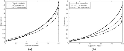
In Sec. 4, through an exhaustive simulation study, we show that our proposed DTEC estimator outperforms the DT estimator in terms of several statistical performance measures including those for graphical models.

3. Penalty parameter selection

The performance of the estimated precision matrix greatly depends on the penalty parameter. Moreover, the penalty parameter controls the sparsity pattern of the estimated matrix. In this article, we suggest the use of a criterion based on the log-likelihood function of the Gaussian model. We define the score function as (5) $$\text{SF}(\tau )=-\hspace{0.17em}\text{log}\hspace{0.17em}\det \widehat{\Omega }(\tau )+\text{trace}\left(S\widehat{\Omega }\right(\tau \left)\right)+\mathrm{k}\times \text{nz}(\tau ),$$(5) where $\text{nz}(\tau )=\text{card}\{(i,j):1\le i\le j\le p,{[\widehat{\Omega }(\tau )]}_{\mathit{ij}}\cancel{=}0\}$ and $\mathrm{k}$ is degrees of freedom. We select the parameter by $\widehat{\tau }=\arg {\min }_{\tau }\text{SF}(\tau ).$ The advantage of the suggested criterion is twofold. First, it is more effective than the techniques based on the cross-validation in terms of the computational time. Second, it accounts the sparsity characteristics of $\widehat{\Omega }.$ Further, we consider the following degrees of freedom: (6) $${\mathrm{k}}_{\text{BIC}}=\frac{\hspace{0.17em}\text{log}\hspace{0.17em}n}{n},$$(6) (7) $${\mathrm{k}}_{\text{HQIC}}=\frac{2\hspace{0.17em}\text{log}\hspace{0.17em}\hspace{0.17em}\text{log}\hspace{0.17em}n}{n}.$$(7)

The choice ${\mathrm{k}}_{\text{BIC}}$ corresponds to the Bayesian Information Criterion (BIC) which is proposed by Yuan and Lin (2007) for precision matrix estimation methodologies. On the other hand, the choice ${\mathrm{k}}_{\text{HQIC}}$ corresponds to the Hannan-Quinn Information Criterion (HQIC) (Hannan and Quinn 1979), which is consistent and asymptotically well-behaved (van der Pas and Grünwald 2014). This is a novel criterion in this framework (to the best of our knowledge, it has not been employed for selecting the penalty terms of the precision matrix estimation methods) and a little attention has been paid to the HQIC, in general.

We note that our proposed methodology requires selection of two parameters, τ and γ. For this reason, we define the following multivariate score function to select these parameters simultaneously: (8) $$\text{MSF}(\tau ,\gamma )=-\hspace{0.17em}\text{log}\hspace{0.17em}\det \widehat{\Omega }(\tau ,\gamma )+\text{trace}\left(S\widehat{\Omega }\right(\tau ,\gamma \left)\right)+\mathrm{k}\times \text{nz}(\tau ),$$(8) where $\widehat{\Omega }(\tau ,\gamma )$ is the estimated precision matrix for given values τ and γ. We select the parameters $\widehat{\tau }$ and $\widehat{\gamma }$ by $(\widehat{\tau },\widehat{\gamma })=\arg {\min }_{\tau ,\gamma }\text{MSF}(\tau ,\gamma ).$

4. Simulation study

In this section, we conduct a simulation analysis to evaluate the performance of our proposed methodology. In Sec. 4.1, we detail the considered models (i.e., patterns) for the true precision matrix Ω. In Sec. 4.2, we describe the performance evaluation. Finally, in subsection 4.3, we provide the discussion of the results.

4.1. Considered models

We perform a simulation study through six different patterns for the precision matrix with varying sizes. The considered models for the matrix Ω are the following:

1. Deterministic patterns

2. Model 1. Tridiagonal design: ${\omega }_{\mathit{ii}}=1,{\omega }_{i,i-1}={\omega }_{i-1,i}=0.45$ and others are 0.

3. Model 2. Tridiagonal design with varying entries: $\Omega =D^{1/2}{\Omega }_1{D}^{1/2},$ where D is a diagonal matrix with entries $D_{\mathit{ii}}=\frac{4i+p-5}{5(p-1)},i=1,\dots ,p$ and ${\Omega }_1$ is a matrix defined in the Model 1.

4. Model 3. Light-tailed (decaying) design: ${\omega }_{\mathit{ij}}={0.6}^{|i-j|}.$

5. Model 4. A block-diagonal matrix, with four equally sized blocks along the diagonal, with a light-tailed model in each block.

6. Random patterns (generated using the MATLAB command sprandsym)

7. Model 5. A random p.d. matrix, with approximately 20% of non-zero entries.

8. Model 6. A random p.d. matrix, with approximately 50% of non-zero entries.

For each precision matrix model, we simulate multivariate normal random samples with zero mean. We set n = 100 and p = 100, 200 and 300. The number of replications is 100.

4.2. Performance evaluation

To evaluate the performance of a precision matrix estimator, we use several losses and measures. In particular, we consider the Kullback–Leibler loss (KLL) and the Reverse Kullback–Leibler loss (RKLL), defined as (9) $$\text{KLL}(\widehat{\Omega },\Omega )=\text{trace}\left({\Omega }^{-1}\widehat{\Omega }\right)-\hspace{0.17em}\text{log}\hspace{0.17em}\det \left({\Omega }^{-1}\widehat{\Omega }\right)-p,$$(9) (10) $$\text{RKLL}(\widehat{\Omega },\Omega )=\text{trace}(\Omega {\widehat{\Omega }}^{-1})-\hspace{0.17em}\text{log}\hspace{0.17em}\det (\Omega {\widehat{\Omega }}^{-1})-p,$$(10) respectively. We also consider matrix losses: the Frobenius norm, the spectral norm and the matrix ${\ell }_1$ norm, defined respectively as (11) $${\ell }_2(\widehat{\Omega },\Omega )=\left|\right|\widehat{\Omega }-\Omega |{|}_2,$$(11) (12) $${\ell }_{\text{sp}}(\widehat{\Omega },\Omega )=\left|\right|\widehat{\Omega }-\Omega |{|}_{\text{sp}},$$(12) (13) $${\ell }_1(\widehat{\Omega },\Omega )=\left|\right|\widehat{\Omega }-\Omega |{|}_{{\ell }_1}.$$(13)

In order to evaluate the sparsity pattern of the precision matrix estimator (i.e., GGM selection performance), we compute Specificity, Sensitivity, Matthews Correlation Coefficient (Matthews 1975) and F₁ score (Powers 2011), defined as (14) $$\text{Specificity}=\frac{\text{TN}}{\text{TN}+\text{FP}},$$(14) (15) $$\text{Sensitivity}=\frac{\text{TP}}{\text{TP}+\text{FN}},$$(15) (16) $$\text{MCC}=\frac{\text{TP}\times \text{TN}-\text{FP}\times \text{FN}}{\sqrt{(\text{TP}+\text{FP})(\text{TP}+\text{FN})(\text{TN}+\text{FP})(\text{TN}+\text{FN})}},$$(16) (17) $${\mathrm{F}}_1=2\frac{\text{Precision}\times \text{Recall}}{\text{Precision}+\text{Recall}},$$(17) where TP, TN, FP and FN are the number of correctly estimated non-zero entries (true positives), the number of correctly estimated zero entries (true negatives), the number of incorrectly estimated non-zero entries (false positives) and the number of incorrectly estimated zero entries (false negatives), respectively. In (17), we define $\text{Precision}=\text{TP}/(\text{TP}+\text{FP})$ and $\text{Recall}=\text{TP}/(\text{TP}+\text{FN}).$ The values of MCC are in [-1,1], and the closer the MCC to one is, the better the classification is. On the other hand, the values of F₁ score are in [0,1], and the closer the F₁ to one is, the better the classification is. It is worth to note that both MCC and F₁ are commonly used to evaluate the performance of binary classifiers (in our context, we consider these measures for the overall evaluation of the GGM selection). However, we put MCC above F₁ score, because MCC takes into account all four classification categories (thus, it is more informative), whereas F₁ score highly depends on the specification of positive categories (Chicco 2017).

We compare our proposed estimator with DT and GLASSO. We select the penalty parameters of these methods using univariate BIC and HQIC criteria. On the other hand, the parameters τ and γ of the proposed estimator DTEC are selected using multivariate BIC and HQIC criteria. Moreover, since the trace of the estimated matrix decreases when τ increases, we consider $\gamma =\tau$ in the proposed problem (3) as a naive case. We call the obtained estimator simplified DTEC or SDTEC, which is defined as the solution of the following optimization problem: (18) $${\widehat{\Omega }}_{\text{SDTEC}}=\arg \underset{\Omega \succcurlyeq ϵI}{\min }\frac{1}{2}\text{trace}\left({\Omega }^{2}S\right)-(1+\tau )\text{trace}(\Omega )+\tau \left|\right|\Omega |{|}_1.$$(18)

In this way, we can calibrate only one parameter instead of two, which leads to saving the computational time.

4.3. Discussion of results

Tables 1–6 summarize the simulation results. Each table reports the averages over 100 replications and the standard deviations of the corresponding measures. We organize the discussion of our results as follows. First, we compare our proposed estimator DTEC with DT and GLASSO estimators when the penalty parameters are selected using the BIC approach. Next, we discuss the same comparison when the parameters are selected using the HQIC approach. Finally, we compare BIC and HQIC approaches through the corresponding measures.

Table 1. Average measures (with standard deviations) over 100 replications for Model 1.

		BIC				HQIC
	p	DT	DTEC	SDTEC	GLASSO	DT	DTEC	SDTEC	GLASSO
	100	10.68 (0.61)	10.82 (1.03)	10.67 (1.24)	18.95 (1.38)	8.94 (0.62)	9.43 (0.68)	9.41 (0.66)	14.14 (1.11)
KLL	200	31.07 (1.15)	24.92 (1.22)	25.05 (1.19)	49.43 (1.90)	23.23 (0.88)	22.76 (1.05)	22.88 (1.03)	39.96 (3.29)
	300	46.62 (1.14)	38.66 (1.53)	38.12 (1.28)	81.80 (4.85)	35.41 (1.05)	35.66 (1.25)	35.51 (1.25)	68.39 (4.64)
	100	13.32 (0.87)	9.18 (0.69)	8.84 (1.23)	31.91 (2.92)	10.28 (0.88)	7.66 (0.61)	7.55 (0.48)	21.58 (2.30)
RKLL	200	43.52 (1.90)	20.54 (1.35)	21.09 (0.99)	90.22 (4.41)	29.11 (1.28)	17.49 (1.10)	18.70 (0.82)	67.97 (7.58)
	300	64.93 (2.07)	33.28 (2.89)	31.64 (1.02)	154.36 (12.41)	43.36 (1.43)	29.10 (1.68)	28.47 (0.92)	121.38 (11.46)
	100	4.77 (0.13)	3.64 (0.24)	3.51 (0.31)	6.76 (0.18)	4.19 (0.17)	3.22 (0.23)	3.17 (0.13)	5.90 (0.25)
${\ell }_2$	200	8.21 (0.13)	5.40 (0.28)	5.54 (0.15)	10.52 (0.14)	6.99 (0.13)	4.76 (0.29)	5.13 (0.14)	9.70 (0.33)
	300	10.03 (0.11)	6.98 (0.42)	6.74 (0.13)	13.31 (0.27)	8.49 (0.12)	6.38 (0.32)	6.26 (0.13)	12.49 (0.31)
	100	1.18 (0.04)	1.03 (0.06)	1.02 (0.06)	1.40 (0.03)	1.15 (0.06)	0.99 (0.07)	0.98 (0.07)	1.39 (0.04)
${\ell }_1$	200	1.30 (0.03)	1.08 (0.05)	1.09 (0.05)	1.46 (0.02)	1.24 (0.05)	1.04 (0.06)	1.07 (0.06)	1.48 (0.04)
	300	1.30 (0.03)	1.11 (0.05)	1.10 (0.04)	1.49 (0.02)	1.27 (0.04)	1.10 (0.05)	1.10 (0.05)	1.52 (0.03)
	100	0.98 (0.03)	0.82 (0.05)	0.80 (0.05)	1.21 (0.02)	0.89 (0.04)	0.75 (0.05)	0.74 (0.05)	1.10 (0.03)
${\ell }_{\text{sp}}$	200	1.13 (0.02)	0.87 (0.04)	0.88 (0.03)	1.30 (0.01)	1.02 (0.03)	0.81 (0.04)	0.84 (0.04)	1.23 (0.03)
	300	1.13 (0.02)	0.91 (0.04)	0.89 (0.03)	1.34 (0.02)	1.03 (0.02)	0.87 (0.04)	0.86 (0.03)	1.28 (0.02)
	100	1 (0)	1 (0)	1 (0)	1 (0)	1 (0)	1 (0)	1 (0)	1 (0)
Sens	200	1 (0)	1 (0)	1 (0)	1 (0)	1 (0)	1 (0)	1 (0)	1 (0)
	300	1 (0)	1 (0)	1 (0)	1 (0)	1 (0)	1 (0)	1 (0)	1 (0)
	100	0.971 (0.002)	0.981 (0.005)	0.977 (0.009)	0.945 (0.009)	0.944 (0.006)	0.964 (0.006)	0.963 (0.002)	0.898 (0.015)
Spec	200	0.995 (0.0005)	0.992 (0.001)	0.992 (0.0006)	0.978 (0.003)	0.981 (0.001)	0.984 (0.003)	0.987 (0.001)	0.957 (0.009)
	300	0.995 (0.0003)	0.993 (0.001)	0.993 (0.0003)	0.987 (0.003)	0.982 (0.0007)	0.988 (0.001)	0.987 (0.0006)	0.974 (0.005)
	100	0.710 (0.016)	0.787 (0.047)	0.764 (0.080)	0.585 (0.035)	0.581 (0.031)	0.669 (0.033)	0.665 (0.015)	0.460 (0.029)
MCC	200	0.871 (0.012)	0.795 (0.023)	0.818 (0.012)	0.640 (0.026)	0.667 (0.012)	0.697 (0.035)	0.734 (0.013)	0.508 (0.044)
	300	0.834 (0.009)	0.787 (0.030)	0.767 (0.009)	0.664 (0.042)	0.595 (0.008)	0.679 (0.025)	0.669 (0.008)	0.530 (0.046)
	100	0.683 (0.019)	0.772 (0.054)	0.745 (0.091)	0.532 (0.043)	0.527 (0.038)	0.634 (0.041)	0.629 (0.018)	0.381 (0.034)
F1	200	0.865 (0.013)	0.795 (0.027)	0.805 (0.014)	0.590 (0.033)	0.624 (0.014)	0.661 (0.043)	0.706 (0.015)	0.425 (0.054)
	300	0.823 (0.010)	0.767 (0.036)	0.745 (0.010)	0.617 (0.053)	0.530 (0.010)	0.636 (0.032)	0.623 (0.011)	0.448 (0.059)

Table 2. Average measures (with standard deviations) over 100 replications for Model 2.

		BIC				HQIC
	p	DT	DTEC	SDTEC	GLASSO	DT	DTEC	SDTEC	GLASSO
	100	11.59 (0.56)	11.34 (0.82)	11.26 (0.72)	20.72 (1.58)	9.47 (0.87)	10.12 (0.80)	10.02 (0.69)	15.42 (1.22)
KLL	200	30.95 (1.20)	27.00 (1.34)	27.62 (1.18)	56.26 (1.40)	23.57 (0.84)	23.80 (1.11)	23.74 (1.09)	43.11 (3.37)
	300	46.77 (1.07)	42.42 (1.44)	42.30 (1.42)	95.97 (2.85)	36.36 (2.39)	37.62 (2.10)	37.45 (2.04)	75.74 (4.01)
	100	14.80 (0.80)	9.46 (1.02)	9.36 (0.55)	37.27 (3.83)	10.77 (1.51)	8.06 (0.74)	7.87 (0.57)	24.48 (2.81)
RKLL	200	43.04 (2.09)	22.00 (1.69)	23.50 (1.13)	113.36 (3.82)	28.90 (1.21)	18.60 (1.09)	18.97 (0.79)	77.13 (9.03)
	300	64.52 (1.85)	35.95 (1.57)	35.61 (1.04)	204.31 (8.71)	43.31 (4.54)	31.38 (1.85)	29.26 (2.04)	143.87 (11.53)
	100	3.21 (0.09)	2.36 (0.21)	2.36 (0.10)	4.83 (0.12)	2.71 (0.19)	2.09 (0.17)	2.05 (0.11)	4.25 (0.16)
${\ell }_2$	200	5.24 (0.11)	3.57 (0.21)	3.76 (0.13)	7.53 (0.05)	4.43 (0.11)	3.18 (0.18)	3.26 (0.11)	6.85 (0.20)
	300	6.41 (0.08)	4.65 (0.14)	4.62 (0.09)	9.56 (0.08)	5.36 (0.24)	4.28 (0.23)	4.00 (0.21)	8.85 (0.15)
	100	1.04 (0.06)	0.86 (0.08)	0.86 (0.07)	1.44 (0.03)	0.99 (0.08)	0.84 (0.09)	0.83 (0.08)	1.36 (0.04)
${\ell }_1$	200	1.17 (0.05)	0.95 (0.07)	0.98 (0.06)	1.54 (0.01)	1.09 (0.08)	0.90 (0.09)	0.91 (0.09)	1.46 (0.03)
	300	1.18 (0.05)	0.99 (0.06)	0.99 (0.06)	1.57 (0.01)	1.12 (0.06)	0.97 (0.07)	0.95 (0.07)	1.51 (0.02)
	100	0.88 (0.05)	0.70 (0.07)	0.70 (0.06)	1.32 (0.03)	0.78 (0.07)	0.64 (0.07)	0.63 (0.06)	1.20 (0.04)
${\ell }_{\text{sp}}$	200	1.02 (0.05)	0.77 (0.06)	0.80 (0.05)	1.46 (0.01)	0.89 (0.06)	0.70 (0.07)	0.72 (0.06)	1.36 (0.03)
	300	1.02 (0.04)	0.81 (0.04)	0.81 (0.04)	1.51 (0.01)	0.90 (0.05)	0.77 (0.06)	0.73 (0.06)	1.43 (0.02)
	100	1 (0)	1 (0)	1 (0)	0.996 (0.004)	1 (0)	1 (0)	1 (0)	0.999 (0.001)
Sens	200	1 (0)	1 (0)	1 (0)	0.990 (0.005)	1 (0)	1 (0)	1 (0)	0.998 (0.001)
	300	1 (0)	1 (0)	1 (0)	0.979 (0.007)	1 (0)	1 (0)	1 (0)	0.996 (0.003)
	100	0.972 (0.002)	0.980 (0.004)	0.980 (0.002)	0.933 (0.010)	0.936 (0.014)	0.958 (0.009)	0.955 (0.007)	0.880 (0.017)
Spec	200	0.992 (0.001)	0.991 (0.002)	0.992 (0.001)	0.972 (0.002)	0.974 (0.001)	0.981 (0.002)	0.982 (0.001)	0.941 (0.009)
	300	0.992 (0.0004)	0.993 (0.0006)	0.993 (0.0004)	0.983 (0.002)	0.975 (0.004)	0.986 (0.003)	0.983 (0.003)	0.963 (0.004)
	100	0.719 (0.017)	0.776 (0.034)	0.772 (0.018)	0.544 (0.032)	0.558 (0.060)	0.642 (0.046)	0.627 (0.041)	0.426 (0.030)
MCC	200	0.812 (0.022)	0.797 (0.036)	0.824 (0.028)	0.581 (0.017)	0.602 (0.010)	0.657 (0.023)	0.666 (0.011)	0.443 (0.0357)
	300	0.763 (0.010)	0.785 (0.016)	0.781 (0.010)	0.596 (0.019)	0.536 (0.047)	0.650 (0.041)	0.612 (0.054)	0.456 (0.028)
	100	0.694 (0.020)	0.761 (0.039)	0.756 (0.021)	0.482 (0.039)	0.498 (0.073)	0.600 (0.055)	0.582 (0.049)	0.343 (0.034)
F1	200	0.798 (0.026)	0.780 (0.042)	0.812 (0.033)	0.518 (0.021)	0.543 (0.012)	0.611 (0.029)	0.623 (0.014)	0.346 (0.043)
	300	0.739 (0.013)	0.765 (0.018)	0.761 (0.012)	0.536 (0.025)	0.455 (0.059)	0.599 (0.051)	0.551 (0.067)	0.356 (0.036)

Table 3. Average measures (with standard deviations) over 100 replications for Model 3.

		BIC				HQIC
	p	DT	DTEC	SDTEC	GLASSO	DT	DTEC	SDTEC	GLASSO
	100	15.75 (0.51)	15.36 (1.04)	15.38 (1.21)	22.98 (0.72)	13.74 (0.41)	14.19 (0.69)	14.17 (0.68)	20.78 (0.68)
KLL	200	34.09 (0.73)	33.40 (1.06)	33.41 (0.99)	50.60 (1.09)	33.30 (2.05)	30.52 (1.14)	30.36 (1.13)	46.51 (1.63)
	300	51.30 (1.43)	51.72 (1.32)	50.76 (1.08)	81.73 (1.97)	51.13 (0.92)	50.20 (1.42)	50.57 (1.13)	75.77 (0.50)
	100	36.58 (1.75)	27.02 (1.87)	27.02 (3.49)	64.83 (3.02)	28.74 (1.23)	22.43 (2.12)	23.20 (2.28)	55.48 (2.78)
RKLL	200	82.40 (2.42)	60.70 (3.75)	61.39 (1.90)	150.16 (4.85)	78.86 (8.90)	52.59 (3.11)	49.66 (3.62)	131.92 (7.13)
	300	122.81 (5.61)	100.01 (6.10)	91.82 (2.17)	252.30 (9.36)	122.47 (3.12)	84.75 (4.95)	91.86 (2.36)	224.33 (2.05)
	100	10.34 (0.08)	9.65 (0.15)	9.63 (0.28)	11.41 (0.06)	9.84 (0.09)	9.20 (0.25)	9.29 (0.29)	11.14 (0.07)
${\ell }_2$	200	14.99 (0.07)	14.04 (0.20)	14.08 (0.08)	16.51 (0.06)	14.84 (0.38)	13.59 (0.21)	13.38 (0.22)	16.21 (0.11)
	300	18.35 (0.12)	17.57 (0.24)	17.24 (0.08)	20.53 (0.10)	18.34 (0.08)	16.89 (0.24)	17.24 (0.09)	20.23 (0.02)
	100	3.48 (0.04)	3.37 (0.05)	3.36 (0.05)	3.58 (0.02)	3.42 (0.04)	3.31 (0.05)	3.32 (0.05)	3.59 (0.03)
${\ell }_1$	200	3.54 (0.03)	3.43 (0.04)	3.44 (0.04)	3.64 (0.02)	3.53 (0.03)	3.41 (0.04)	3.40 (0.04)	3.65 (0.03)
	300	3.56 (0.03)	3.48 (0.03)	3.46 (0.03)	3.65 (0.01)	3.56 (0.03)	3.44 (0.03)	3.46 (0.03)	3.66 (0.02)
	100	3.22 (0.02)	3.07 (0.04)	3.06 (0.06)	3.44 (0.01)	3.11 (0.02)	2.96 (0.06)	2.98 (0.06)	3.38 (0.01)
${\ell }_{\text{sp}}$	200	3.29 (0.01)	3.14 (0.03)	3.15 (0.02)	3.49 (0.01)	3.26 (0.06)	3.07 (0.03)	3.03 (0.04)	3.45 (0.01)
	300	3.29 (0.02)	3.19 (0.03)	3.15 (0.02)	3.53 (0.01)	3.29 (0.01)	3.10 (0.03)	3.15 (0.02)	3.50 (0.003)
	100	0.047 (0.001)	0.043 (0.005)	0.045 (0.008)	0.046 (0.003)	0.070 (0.002)	0.060 (0.012)	0.059 (0.015)	0.067 (0.006)
Sens	200	0.025 (0.0007)	0.021 (0.001)	0.021 (0.0006)	0.022 (0.001)	0.029 (0.009)	0.032 (0.004)	0.035 (0.005)	0.032 (0.003)
	300	0.020 (0.001)	0.014 (0.001)	0.016 (0.0004)	0.012 (0.001)	0.020 (0.0005)	0.018 (0.002)	0.016 (0.0004)	0.017 (0.0008)
	100	NA (NA)	NA (NA)	NA (NA)	NA (NA)	NA (NA)	NA (NA)	NA (NA)	NA (NA)
Spec	200	NA (NA)	NA (NA)	NA (NA)	NA (NA)	NA (NA)	NA (NA)	NA (NA)	NA (NA)
	300	NA (NA)	NA (NA)	NA (NA)	NA (NA)	NA (NA)	NA (NA)	NA (NA)	NA (NA)
	100	NA (NA)	NA (NA)	NA (NA)	NA (NA)	NA (NA)	NA (NA)	NA (NA)	NA (NA)
MCC	200	NA (NA)	NA (NA)	NA (NA)	NA (NA)	NA (NA)	NA (NA)	NA (NA)	NA (NA)
	300	NA (NA)	NA (NA)	NA (NA)	NA (NA)	NA (NA)	NA (NA)	NA (NA)	NA (NA)
	100	0.090 (0.003)	0.083 (0.009)	0.086 (0.015)	0.088 (0.006)	0.131 (0.004)	0.113 (0.021)	0.111 (0.026)	0.126 (0.012)
F1	200	0.049 (0.001)	0.042 (0.002)	0.041 (0.001)	0.043 (0.003)	0.056 (0.018)	0.062 (0.008)	0.069 (0.009)	0.062 (0.007)
	300	0.039 (0.002)	0.029 (0.002)	0.032 (0.0007)	0.025 (0.002)	0.039 (0.001)	0.036 (0.003)	0.032 (0.0008)	0.034 (0.001)

Spec and MCC are excluded for model 3, because these measurements are not defined for dense models.

Table 4. Average measures (with standard deviations) over 100 replications for Model 4.

		BIC				HQIC
	p	DT	DTEC	SDTEC	GLASSO	DT	DTEC	SDTEC	GLASSO
	100	16.30 (0.87)	14.95 (0.89)	15.04 (1.11)	22.60 (0.70)	13.34 (0.43)	13.76 (0.66)	13.81 (0.57)	20.30 (0.74)
KLL	200	33.45 (0.70)	32.81 (0.81)	32.81 (0.77)	50.07 (0.33)	33.13 (1.58)	29.90 (1.00)	29.99 (1.28)	45.91 (1.17)
	300	50.87 (2.20)	50.87 (1.39)	49.88 (1.07)	80.98 (2.57)	50.40 (0.82)	49.56 (1.10)	49.77 (1.15)	75.33 (0.94)
	100	38.63 (3.35)	25.97 (1.98)	26.27 (3.16)	62.60 (2.81)	27.41 (1.23)	21.54 (1.86)	22.44 (1.77)	53.10 (2.97)
RKLL	200	79.96 (2.53)	59.01 (3.29)	59.50 (1.85)	147.07 (1.35)	78.35 (7.20)	51.97 (2.60)	48.86 (4.40)	128.79 (5.14)
	300	121.68 (8.59)	97.93 (5.57)	90.04 (2.26)	247.89 (11.87)	119.69 (2.68)	82.66 (4.39)	89.30 (3.37)	221.61 (4.06)
	100	10.24 (0.19)	9.37 (0.17)	9.38 (0.26)	11.15 (0.06)	9.55 (0.09)	8.93 (0.23)	9.04 (0.23)	10.86 (0.09)
${\ell }_2$	200	14.77 (0.08)	13.81 (0.18)	13.85 (0.09)	16.32 (0.01)	14.70 (0.33)	13.44 (0.19)	13.19 (0.27)	16.01 (0.08)
	300	18.20 (0.19)	17.39 (0.22)	17.06 (0.09)	20.37 (0.13)	18.16 (0.08)	16.69 (0.22)	17.03 (0.17)	20.08 (0.05)
	100	3.47 (0.04)	3.33 (0.05)	3.33 (0.06)	3.56 (0.02)	3.39 (0.04)	3.27 (0.06)	3.29 (0.05)	3.56 (0.03)
${\ell }_1$	200	3.53 (0.02)	3.43 (0.03)	3.43 (0.03)	3.62 (0.01)	3.53 (0.03)	3.41 (0.05)	3.39 (0.05)	3.63 (0.02)
	300	3.56 (0.03)	3.48 (0.03)	3.45 (0.04)	3.65 (0.01)	3.56 (0.03)	3.43 (0.04)	3.46 (0.04)	3.66 (0.02)
	100	3.14 (0.04)	2.95 (0.04)	2.95 (0.06)	3.29 (0.01)	3,00 (0.03)	2.85 (0.06)	2.88 (0.06)	3.24 (0.02)
${\ell }_{\text{sp}}$	200	3.25 (0.01)	3.11 (0.03)	3.11 (0.02)	3.45 (0.005)	3.24 (0.05)	3.05 (0.03)	3.01 (0.05)	3.41 (0.01)
	300	3.28 (0.02)	3.18 (0.03)	3.13 (0.02)	3.51 (0.01)	3.27 (0.02)	3.08 (0.04)	3.13 (0.03)	3.48 (0.008)
	100	0.132 (0.009)	0.133 (0.009)	0.134 (0.012)	0.130 (0.005)	0.170 (0.006)	0.155 (0.014)	0.151 (0.015)	0.150 (0.009)
Sens	200	0.070 (0.001)	0.066 (0.001)	0.066 (0.001)	0.064 (0.001)	0.073 (0.009)	0.079 (0.005)	0.083 (0.007)	0.075 (0.003)
	300	0.050 (0.002)	0.044 (0.001)	0.046 (0.0007)	0.040 (0.001)	0.051 (0.001)	0.049 (0.002)	0.047 (0.003)	0.045 (0.005)
	100	0.988 (0.005)	0.987 (0.004)	0.987 (0.007)	0.982 (0.003)	0.962 (0.003)	0.973 (0.010)	0.976 (0.011)	0.960 (0.008)
Spec	200	0.990 (0.0007)	0.993 (0.001)	0.993 (0.0006)	0.992 (0.001)	0.988 (0.008)	0.984 (0.003)	0.981 (0.005)	0.981 (0.003)
	300	0.990 (0.001)	0.995 (0.0009)	0.993 (0.0004)	0.996 (0.001)	0.990 (0.001)	0.992 (0.002)	0.993 (0.002)	0.991 (0.001)
	100	0.262 (0.011)	0.261 (0.012)	0.262 (0.012)	0.234 (0.011)	0.224 (0.011)	0.237 (0.016)	0.240 (0.015)	0.194 (0.016)
MCC	200	0.168 (0.005)	0.178 (0.005)	0.179 (0.004)	0.167 (0.005)	0.164 (0.013)	0.155 (0.008)	0.150 (0.013)	0.140 (0.009)
	300	0.126 (0.007)	0.143 (0.005)	0.137 (0.003)	0.142 (0.006)	0.125 (0.004)	0.130 (0.006)	0.136 (0.005)	0.124 (0.004)
	100	0.227 (0.011)	0.228 (0.011)	0.229 (0.015)	0.220 (0.006)	0.265 (0.008)	0.251 (0.014)	0.246 (0.014)	0.237 (0.009)
F1	200	0.128 (0.002)	0.122 (0.002)	0.121 (0.002)	0.119 (0.002)	0.132 (0.012)	0.139 (0.007)	0.145 (0.010)	0.133 (0.005)
	300	0.093 (0.003)	0.084 (0.002)	0.087 (0.001)	0.077 (0.002)	0.094 (0.002)	0.091 (0.003)	0.088 (0.004)	0.085 (0.002)

Table 5. Average measures (with standard deviations) over 100 replications for Model 5.

		BIC				HQIC
	p	DT	DTEC	SDTEC	GLASSO	DT	DTEC	SDTEC	GLASSO
	100	13.31 (0.57)	12.24 (0.89)	12.31 (0.85)	23.60 (1.46)	10.85 (0.50)	10.74 (0.68)	10.70 (0.58)	18.88 (1.18)
KLL	200	37.39 (2.16)	33.20 (1.48)	33.40 (1.63)	61.96 (2.50)	31.80 (1.57)	29.98 (0.91)	29.89 (0.83)	52.96 (2.65)
	300	60.49 (0.88)	55.62 (1.65)	55.45 (1.63)	98.60 (3.20)	52.01 (0.88)	51.28 (1.23)	51.20 (1.06)	88.28 (2.93)
	100	27.05 (1.96)	18.55 (2.18)	18.62 (2.24)	59.02 (5.66)	18.63 (1.36)	13.55 (1.25)	13.55 (1.22)	40.76 (4.44)
RKLL	200	84.32 (7.61)	52.24 (3.82)	52.55 (4.21)	175.09 (11.44)	64.22 (6.25)	41.93 (2.78)	42.13 (2.04)	135.28 (11.54)
	300	157.43 (4.16)	105.24 (6.54)	104.93 (5.40)	301.02 (15.68)	120.35 (3.04)	87.20 (5.30)	88.53 (2.66)	251.68 (13.73)
	100	1.83 (0.04)	1.58 (0.06)	1.58 (0.06)	2.65 (0.05)	1.63 (0.05)	1.44 (0.06)	1.44 (0.06)	2.44 (0.07)
${\ell }_2$	200	2.94 (0.08)	2.54 (0.06)	2.54 (0.07)	3.97 (0.04)	2.70 (0.09)	2.37 (0.07)	2.37 (0.06)	3.79 (0.07)
	300	3.74 (0.04)	3.39 (0.07)	3.39 (0.07)	4.94 (0.04)	3.53 (0.13)	3.31 (0.15)	3.31 (0.14)	4.79 (0.05)
	100	1.25 (0.03)	1.21 (0.05)	1.21 (0.05)	1.47 (0.02)	1.20 (0.04)	1.15 (0.05)	1.15 (0.05)	1.42 (0.02)
${\ell }_1$	200	1.63 (0.05)	1.56 (0.05)	1.56 (0.05)	1.74 (0.01)	1.57 (0.07)	1.50 (0.07)	1.50 (0.06)	1.72 (0.01)
	300	1.84 (0.08)	1.78 (0.14)	1.78 (0.14)	2.05 (0.01)	1.83 (0.46)	1.77 (0.39)	1.77 (0.38)	2.04 (0.01)
	100	0.76 (0.02)	0.73 (0.03)	0.73 (0.03)	0.84 (0.01)	0.72 (0.03)	0.68 (0.03)	0.68 (0.03)	0.80 (0.01)
${\ell }_{\text{sp}}$	200	0.90 (0.01)	0.87 (0.02)	0.87 (0.02)	0.92 (0.00)	0.87 (0.02)	0.84 (0.02)	0.84 (0.02)	0.90 (0.01)
	300	0.85 (0.06)	0.83 (0.13)	0.83 (0.12)	0.89 (0.01)	0.87 (0.24)	0.87 (0.25)	0.86 (0.25)	0.88 (0.01)
	100	0.144 (0.006)	0.131 (0.011)	0.131 (0.011)	0.156 (0.015)	0.183 (0.011)	0.167 (0.014)	0.167 (0.012)	0.212 (0.020)
Sens	200	0.068 (0.007)	0.062 (0.005)	0.062 (0.006)	0.065 (0.005)	0.088 (0.010)	0.082 (0.005)	0.082 (0.004)	0.091 (0.011)
	300	0.043 (0.001)	0.037 (0.002)	0.037 (0.002)	0.046 (0.003)	0.059 (0.002)	0.049 (0.003)	0.048 (0.002)	0.060 (0.006)
	100	0.980 (0.002)	0.986 (0.005)	0.987 (0.005)	0.957 (0.009)	0.954 (0.007)	0.966 (0.008)	0.965 (0.007)	0.912 (0.017)
Spec	200	0.991 (0.004)	0.994 (0.002)	0.994 (0.002)	0.982 (0.004)	0.979 (0.008)	0.983 (0.003)	0.983 (0.003)	0.962 (0.009)
	300	0.992 (0.0005)	0.995 (0.0009)	0.995 (0.0008)	0.989 (0.002)	0.981 (0.001)	0.989 (0.002)	0.989 (0.001)	0.980 (0.004)
	100	0.240 (0.011)	0.249 (0.012)	0.249 (0.013)	0.184 (0.013)	0.210 (0.014)	0.222 (0.014)	0.221 (0.014)	0.156 (0.015)
MCC	200	0.165 (0.008)	0.170 (0.006)	0.170 (0.007)	0.116 (0.009)	0.148 (0.011)	0.153 (0.008)	0.153 (0.007)	0.098 (0.009)
	300	0.114 (0.004)	0.121 (0.004)	0.120 (0.004)	0.105 (0.005)	0.099 (0.005)	0.108 (0.005)	0.109 (0.005)	0.095 (0.005)
	100	0.235 (0.008)	0.221 (0.013)	0.220 (0.013)	0.234 (0.014)	0.267 (0.011)	0.254 (0.014)	0.255 (0.013)	0.268 (0.012)
F1	200	0.123 (0.010)	0.115 (0.008)	0.114 (0.009)	0.115 (0.008)	0.150 (0.011)	0.143 (0.008)	0.142 (0.006)	0.145 (0.012)
	300	0.080 (0.002)	0.069 (0.004)	0.070 (0.004)	0.084 (0.005)	0.104 (0.003)	0.089 (0.005)	0.087 (0.003)	0.104 (0.008)

Table 6. Average measures (with standard deviations) over 100 replications for Model 6.

		BIC				HQIC
	p	DT	DTEC	SDTEC	GLASSO	DT	DTEC	SDTEC	GLASSO
	100	19.67 (1.86)	19.40 (1.11)	19.50 (1.01)	30.42 (1.69)	15.71 (1.31)	16.71 (0.96)	16.78 (0.95)	24.63 (1.36)
KLL	200	46.30 (2.29)	45.63 (1.51)	45.37 (1.41)	70.47 (2.69)	39.99 (1.71)	41.51 (1.39)	41.70 (1.36)	61.12 (2.01)
	300	84.45 (3.63)	77.81 (2.66)	77.58 (3.08)	119.27 (3.64)	74.74 (1.45)	70.72 (1.62)	71.73 (1.12)	106.39 (3.18)
	100	44.73 (7.44)	32.36 (3.44)	32.99 (3.16)	88.30 (8.13)	28.10 (5.37)	23.06 (2.65)	23.25 (3.15)	60.90 (6.18)
RKLL	200	114.93 (10.88)	83.67 (5.63)	83.04 (4.78)	217.72 (13.82)	84.49 (7.47)	67.50 (4.59)	67.04 (6.11)	170.55 (9.83)
	300	234.17 (16.41)	147.95 (9.38)	148.14 (9.74)	383.36 (20.13)	189.14 (8.01)	123.71 (8.36)	126.28 (3.56)	315.08 (16.68)
	100	2.24 (0.10)	2.04 (0.07)	2.05 (0.07)	2.84 (0.04)	1.93 (0.12)	1.79 (0.08)	1.80 (0.09)	2.66 (0.05)
${\ell }_2$	200	3.19 (0.07)	2.95 (0.06)	2.95 (0.06)	4.08 (0.04)	2.95 (0.07)	2.80 (0.07)	2.79 (0.08)	3.92 (0.04)
	300	4.19 (0.08)	3.72 (0.07)	3.72 (0.08)	5.11 (0.04)	3.96 (0.05)	3.53 (0.08)	3.55 (0.05)	4.96 (0.04)
	100	1.56 (0.05)	1.52 (0.05)	1.53 (0.04)	1.78 (0.01)	1.45 (0.06)	1.42 (0.05)	1.42 (0.05)	1.73 (0.02)
${\ell }_1$	200	1.87 (0.02)	1.85 (0.02)	1.85 (0.02)	1.97 (0.01)	1.84 (0.02)	1.83 (0.04)	1.83 (0.03)	1.95 (0.01)
	300	2.09 (0.05)	2.01 (0.03)	2.01 (0.03)	2.29 (0.01)	2.06 (0.04)	1.99 (0.03)	1.99 (0.03)	2.27 (0.01)
	100	0.71 (0.03)	0.67 (0.03)	0.68 (0.03)	0.88 (0.01)	0.63 (0.04)	0.61 (0.03)	0.61 (0.03)	0.84 (0.01)
${\ell }_{\text{sp}}$	200	0.82 (0.01)	0.79 (0.03)	0.79 (0.03)	0.90 (0.006)	0.79 (0.02)	0.77 (0.05)	0.77 (0.04)	0.88 (0.01)
	300	0.85 (0.01)	0.82 (0.03)	0.82 (0.03)	0.90 (0.004)	0.84 (0.01)	0.81 (0.03)	0.81 (0.01)	0.88 (0.01)
	100	0.094 (0.018)	0.079 (0.010)	0.078 (0.010)	0.097 (0.014)	0.155 (0.027)	0.128 (0.018)	0.128 (0.020)	0.161 (0.022)
Sens	200	0.040 (0.004)	0.031 (0.003)	0.031 (0.003)	0.040 (0.005)	0.066 (0.007)	0.049 (0.007)	0.049 (0.009)	0.067 (0.008)
	300	0.022 (0.004)	0.021 (0.003)	0.021 (0.003)	0.025 (0.003)	0.033 (0.003)	0.035 (0.004)	0.031 (0.002)	0.040 (0.005)
	100	0.978 (0.010)	0.986 (0.005)	0.987 (0.005)	0.965 (0.009)	0.934 (0.020)	0.955 (0.012)	0.955 (0.014)	0.917 (0.018)
Spec	200	0.984 (0.004)	0.991 (0.002)	0.991 (0.002)	0.987 (0.003)	0.963 (0.006)	0.977 (0.006)	0.977 (0.007)	0.971 (0.005)
	300	0.994 (0.003)	0.995 (0.002)	0.995 (0.002)	0.991 (0.002)	0.986 (0.003)	0.985 (0.003)	0.987 (0.002)	0.980 (0.004)
	100	0.156 (0.011)	0.157 (0.010)	0.157 (0.010)	0.126 (0.010)	0.144 (0.011)	0.149 (0.010)	0.149 (0.010)	0.121 (0.010)
MCC	200	0.075 (0.007)	0.080 (0.005)	0.080 (0.006)	0.087 (0.006)	0.065 (0.007)	0.072 (0.006)	0.072 (0.006)	0.089 (0.007)
	300	0.072 (0.004)	0.073 (0.003)	0.073 (0.004)	0.063 (0.005)	0.064 (0.004)	0.063 (0.005)	0.065 (0.004)	0.059 (0.005)
	100	0.167 (0.028)	0.145 (0.017)	0.143 (0.017)	0.170 (0.021)	0.251 (0.036)	0.218 (0.025)	0.216 (0.029)	0.257 (0.026)
F1	200	0.075 (0.008)	0.059 (0.005)	0.060 (0.005)	0.076 (0.010)	0.118 (0.012)	0.091 (0.012)	0.092 (0.016)	0.122 (0.013)
	300	0.043 (0.007)	0.040 (0.005)	0.041 (0.006)	0.048 (0.005)	0.063 (0.006)	0.066 (0.007)	0.060 (0.004)	0.076 (0.009)

First, we observe that when the parameters are selected through BIC approach, the estimator DTEC outperforms DT in terms of all statistical losses for almost all the models (except of model 3, in terms of KLL). The estimator DTEC outperforms DT for models 2, 4, 5, 6 in terms of MCC, for model 2 in terms of F₁. On the other hand, DT outperforms DTEC for model 1 in terms of MCC, for models 1, 3, 4, 5, 6 in terms of F₁. Furthermore, we observe that GLASSO provides high statistical losses and low GGM prediction measures.

Second, the results show that when the parameters are selected through HQIC approach, the estimator DTEC outperforms DT in terms of all statistical losses for almost all the models (except of model 2, in terms of KLL). On the other hand, DTEC outperforms DT for models 1, 2, 4, 5 in terms of MCC, for models 1, 2 in terms of F₁. DT method outperforms DTEC for models 3, 4, 5 in terms of F₁. Furthermore, we observe that GLASSO outperforms all the other estimators for model 6 in terms of F₁. However, for the other models GLASSO provides poor results.

Finally, we conduct a comparison BIC and HQIC based on the corresponding losses and measures. We observe, that BIC provides higher statistical losses, whereas HQIC provides lower statistical losses for all considered approaches (including DT and GLASSO methods). Moreover, estimators obtained through BIC provide higher MCC than those for HQIC, and higher F₁ for models 1, 2. Estimators obtained through HQIC provide higher F₁ for models 3, 4, 5, 6 than those for BIC.

In sum, the proposed DTEC estimation method provides better performance than DT and GLASSO methods for most of the models in terms of several statistical losses and GGM prediction measures. Moreover, we observe that this conclusion holds if we consider the simplified SDTEC method (i.e., when $\gamma =\tau$), since it performs as good as DTEC estimator. This finding leads to saving significantly the computational time without sacrificing too much the performance.

5. Real data application

In this section, we conduct an empirical analysis through real-data example. In particular, we focus on the problem of predicting breast cancer patients (subjects) with pathological complete response (pCR) using Linear Discriminant Analysis (LDA). For this application we use a dataset which contains gene expression levels of subjects with different stages of breast cancer. The dataset consists of 22,283 gene expression levels of 271 subjects. There are 58 subjects with pCR and 213 subjects with residual disease (RD). The applied dataset is available in the website of the National Center for Biotechnology Information (http://www.ncbi.nlm.nih.gov/).

First, following the analysis by Cai, Liu, and Luo (2011), we divide the dataset into training and testing sets with sizes 227 and 44 (almost 5/6 and 1/6 of the observations), respectively. For the testing set, we randomly select 9 subjects with pCR and 35 subjects with RD (roughly 1/6 of the subjects in each group). The training set contains the remaining subjects. Second, based on the training set we perform two sample t-tests between two groups and select the most significant 200 genes with the smallest p-values. Third, using the training set, we estimate the precision matrix Ω with the DT, DTEC, SDTEC and GLASSO methods. Finally, we use the estimated precision matrix in the LDA score function, defined as ${\delta }_t(Y)=Y^T\widehat{\Omega }{\widehat{\mu }}_t-\frac{1}{2}{\widehat{\mu }}_t^T\widehat{\Omega }{\widehat{\mu }}_t,$ where t = 1, 2 (t = 1 for pCR and t = 2 for RD) and ${\widehat{\mu }}_t$ is the within group average, calculated using the training data. We classify the subject Y through the classification rule $\widehat{t}=\arg \max {\delta }_t(Y).$ To measure the prediction accuracy, we use Specificity, Sensitivity, MCC and F₁. We consider TP and TN as the number of correctly predicted RD and pCR, respectively, and FP and FN as the number of erroneously predicted RD and pCR, respectively. We repeat this process 100 times. We report the average measurements in Table 7.

Table 7. Average pCR/RD classification measurements over 100 replications.

BIC
Method	Specificity	Sensitivity	MCC	F 1
DT	0.692	0.749	0.378	0.818
DTEC	0.719	0.742	0.392	0.816
SDTEC	0.713	0.744	0.389	0.817
GLASSO	0.461	0.790	0.232	0.816
		HQIC
Method	Specificity	Sensitivity	MCC	F1
DT	0.559	0.787	0.312	0.827
DTEC	0.606	0.778	0.341	0.827
SDTEC	0.606	0.777	0.340	0.826
GLASSO	0.443	0.802	0.231	0.823

Our findings show that for both selection criteria the GLASSO method provides the highest Sensitivity, but it attains the lowest Specificity and MCC. On the other hand, the DTEC approach provides the highest Specificity and dominates all the other estimators in terms of MCC. We note that all methods provide very similar results in terms of the F₁ score. However, as mentioned earlier, we find MCC more informative than F₁ score. The results also show that SDTEC performs as good as the DTEC estimator. Furthermore, we observe that the obtained Specificity and MCC of the considered estimators are higher for BIC than the same for HQIC, whereas the Sensitivity and F₁ of the estimators are higher for HQIC than the same for BIC.

In sum, for the considered application our proposed DTEC method (and its simplified version SDTEC) provides better classification performance than DT and GLASSO approaches. Therefore, employing additional penalization on the estimated precision matrix eigenvalues improves the estimate, even though the true precision matrix eigenvalues are unknown in this example.

6 Conclusions

In this article, we develop a new approach for estimating high dimensional precision matrices, using the ${\ell }_1$ penalization framework. The proposed method imposes a negative trace penalization on the recently introduced DT estimator. The additional penalty term controls the eigenvalues of the precision matrix estimator and diminishes the reduction of its largest eigenvalues. We conduct an extensive simulation study where we use several statistical losses and measures for the estimation evaluation. The results show that our proposed methodology outperforms DT and GLASSO methods for most of the considered scenarios. In line with the popular BIC method we study the performance of another technique based on HQIC for selecting the penalty parameters. In contrast to its little use in practice, HQIC demonstrates lower statistical losses than BIC in the simulation study. Moreover, we illustrate the performance of our proposed approach through an empirical application aimed at predicting the patients with pCR using LDA. Furthermore, we propose a simplified version of our methodology, which leads to saving the computational time without having to sacrifice the performance.

Acknowledgments

The author would like to thank the anonymous referee and the Editor for their helpful comments that led to an improvement of this article.

References

- Avagyan, V., A. M. Alonso, and F. J. Nogales. 2016. D-trace estimation of a precision matrix using adaptive lasso penalties. Advances in Data Analysis and Classification 12 (2):425–47. doi: 10.1007/s11634-016-0272-8.
- Avagyan, V., A. M. Alonso, and F. J. Nogales. 2017. Improving the graphical lasso estimation for the precision matrix through roots of the sample covariance matrix. Journal of Computational and Graphical Statistics 26 (4):865–72. doi: 10.1080/10618600.2017.1340890.
- Banerjee, O., L. El Ghaoui, A. d’Aspremont, and G. Natsoulis. 2006. Convex optimization techniques for fitting sparse gaussian graphical models. Pittsburg. Proceedings of the
- Cai, T., W. Liu, and X. Luo. 2011. A constrained ℓ1 minimization approach to sparse precision matrix estimation. Journal of the American Statistical Association 106 (494):594–607. doi: 10.1198/jasa.2011.tm10155.
- Chicco, D. 2017. Ten quick tips for machine learning in computational biology. BioData Mining 10 (1):35doi: 10.1186/s13040-017-0155-3.
- Dempster, A. 1972. Covariance selection. Biometrics 28 (1):157–75. doi: 10.2307/2528966.
- Fan, J., J. Feng, and Y. Wu. 2009. Network exploration via the adaptive Lasso and Scad penalties. The Annals of Applied Statistics 3(2):521–41. doi: 10.1214/08-AOAS215SUPP.
- Friedman, J., T. Hastie, and R. Tibshirani. 2008. Sparse inverse covariance estimation with the graphical lasso. Biostatistics 9(3):432–41. doi: 10.1093/biostatistics/kxm045.
- Goto, S., and Y. Xu. 2015. Improving mean variance optimization through sparse hedging restrictions. Journal of Financial and Quantitative Analysis 50 (06):1415–41. doi: 10.1017/S0022109015000526.
- Hannan, E. J., and B. G. Quinn. 1979. The determination of the order of an autoregression. Journal of the Royal Statistical Society: Series B 41 (2):190–5. doi: 10.1111/j.2517-6161.1979.tb01072.x.
- Lauritzen, S. 1996. Graphical models. Oxford: Clarendon Press.
- Liu, H., L. Wang, and T. Zhao. 2014. Sparse covariance matrix estimation with eigenvalue constraints. Journal of Computational and Graphical Statistics 23 (2):439–59. doi: 10.1080/10618600.2013.782818.
- Matthews, B. W. 1975. Comparison of the predicted and observed secondary structure of t4 phage lysozyme. Biochimica et Biophysica Acta 405(2):442–51. doi: 10.1016/0005-2795(75)90109-9.
- Maurya, A. 2014. A joint convex penalty for inverse covariance matrix estimation. Computational Statistics & Data Analysis 75:15–27. doi: 10.1016/j.csda.2014.01.015.
- McLachlan, S. 2004. Discriminant analysis and statistical pattern recognition. New York: Willey Interscience.
- Meinshausen, N., and P. Bühlmann. 2006. High-dimensional graphs and variable selection with the lasso. The Annals of Statistics 34 (3):1436–62. doi: 10.1214/009053606000000281.
- Powers, D. M. 2011. Evaluation: from precision, recall and f-measure to roc, informedness, markedness and correlation. Journal of Machine Learning Technologies 2 (1):37–63.
- Rothman, A., P. Bickel, E. Levina, and J. Zhu. 2008. Sparse permutation invariant covariance estimation. Electronic Journal of Statistics 2 (0):494–515. doi: 10.1214/08-EJS176.
- Ryali, S., T. Chen, K. Supekar, and V. Menon. 2012. Estimation of functional connectivity in fMRI data using stability selection-based sparse partial correlation with elastic net penalty. NeuroImage 59(4):3852–61. doi: 10.1016/j.neuroimage.2011.11.054.
- Stifanelli, P. F., T. M. Creanza, R. Anglani, V. C. Liuzzi, S. Mukherjee, F. P. Schena, and N. Ancona. 2013. A comparative study of covariance selection models for the inference of gene regulatory networks. Journal of Biomedical Informatics 46 (5):894–904. doi: 10.1016/j.jbi.2013.07.002.
- Tibshirani, R. 1996. Regression shrinkage and selection via the lasso. Journal of the Royal Statistical Society: Series B 58 (1):267–88. doi: 10.1111/j.2517-6161.1996.tb02080.x.
- van der Pas, S. L., and P. D. Grünwald. 2014. Almost the best of three worlds: Risk, consistency and optional stopping for the switch criterion in single parameter model selection. arXiv Preprint arXiv:1408.5724.
- van Wieringen, W. N., and C. F. Peeters. 2016. Ridge estimation of inverse covariance matrices from high-dimensional data. Computational Statistics & Data Analysis 103:284–303. doi: 10.1016/j.csda.2016.05.012.
- Yuan, M. 2010. High dimensional inverse covariance matrix estimation via linear programming. Journal of Machine Learning Research 11:2261–86.
- Yuan, M., and Y. Lin. 2007. Model selection and estimation in the Gaussian graphical model. Biometrika 94 (1):19–35. doi: 10.1093/biomet/asm018.
- Zerenner, T., P. Friederichs, K. Lehnertz, and A. Hense. 2014. A gaussian graphical model approach to climate networks. Chaos: An Interdisciplinary Journal of Nonlinear Science 24 (2):023103. doi: 10.1063/1.4870402.
- Zhang, T., and H. Zou. 2014. Sparse precision matrix estimation via lasso penalized d-trace loss. Biometrika 88:1–18.