On the trend detection of time-ordered intensity images of point processes on linear networks

Abstract

Spatial point processes on linear networks are increasingly getting attention in different disciplines such as traffic accidents and street crime analysis. Dealing with a set of time-ordered point patterns on a linear network over a period, helps in obtaining a time series of estimated intensity images. In this article, we combine the problem of estimating the intensity and relative risk of point patterns on linear networks with trend detection in time-ordered observations. Taking the temporal autocorrelation between consecutive time-ordered intensity and relative risk images into account, we make use of the Mann–Kendall trend test to look for potential locations in the network where the estimated intensity and/or relative risk show evidence of a monotonic trend. The monthly time-ordered spatial point patterns of fatal traffic accidents and street crimes in the city of London, UK, in the period of January 2013 to December 2017, are used as an application.

Keywords:

• Mann–Kendall trend test
• Relative risk
• Separability
• Spatio-temporal data
• Street crime
• Traffic accident

1. Introduction

The analysis of spatial point patterns on linear networks, e.g. the location of traffic accidents or street crimes, is increasingly receiving scientific interest. Since such locations inherently only live on their corresponding network structure, considering such structure as the support of data instead of a general state space might result in defining a more realistic scenario (Yamada and Thill 2004). Nevertheless, geometrical complexities of linear networks give rise to different mathematical/computational challenges. Thus far, most of the attention is paid to estimating the intensity function of such point processes non-parametrically (Okabe, Satoh, and Sugihara 2009; McSwiggan, Baddeley, and Nair 2016; Moradi, 2018; Moradi, Rodriguez-Cortes, and Mateu 2018; Moradi et al., 2019; Rakshit et al., 2019). Regarding traffic accidents or street crimes data, such locations are usually recorded daily, and their incidence rate may be affected by external events such as different activities of the Town-hall or the Police department, and/or environmental characteristics like physical environment, weather, and so forth (Feng et al. 2016; Hipp, Kim, and Kane 2019). The density/intensity of traffic accidents and/or street crimes may face gradual/sudden changes over time. For instance, new strategies to reduce the crime/accident rate in a particular area might push the corresponding intensity down at a particular area. The efficiency of such strategies to reduce the rate of traffic accidents or street crimes might be then detectable when having a set of time-ordered realizations of the underlying point process.

The problem of trend/change-point detection has been frequently raised within different disciplines such as agronomy, hydrology, geology, climatology, etc. Several proposals have been developed for detecting gradual/sudden distributional changes in time-ordered datasets including non-parametric, parametric, and regression-based methods (Mann 1945; Kendall 1948; Cox and Stuart 1955; Pettitt 1979; Zeileis et al. 2003; Matteson and James 2014; Grundy, Killick, and Mihaylov 2020). A selective review of several change-point detection methods is provided by Truong, Oudre, and Vayatis (2020). The developed proposals were initially considered for time series, and later they are examined for time series of satellite images (Verbesselt et al. 2010; Bullock, Woodcock, and Holden 2020; Militino, Moradi, and Ugarte 2020). In general, since time-ordered datasets usually experience a seasonal behavior, there also exists a technique to decompose time series into trend, seasonal, and reminder components looking for possible changes in both trend and seasonal components individually (Verbesselt et al. 2010). Although these methods demonstrate a reasonably high power of the test, the majority drastically suffer from a high rate of introducing false positives when dealing with highly autocorrelated data. Several modifications have been proposed to reduce the type I error probability of the Mann–Kendall test in the presence of temporal autocorrelation (Kulkarni and von Storch 1995; Hamed and Rao 1998; Von Storch 1999; Yue et al. 2002; Yue and Wang 2004; Hamed 2009). Nevertheless, their major drawback is to reduce the power of the test along with reducing the type I error probability. Note that reducing the power of the test means increasing the type II error probability. It is shown that taking a tradeoff between the type I and II error probabilities into account, the original Mann–Kendall method might still be a reliable technique (Militino, Moradi, and Ugarte 2020).

Although, in practice, this might often be the case to have a set of time-ordered point patterns on a linear network, to the best of our knowledge this field has not yet benefited from trend detection techniques. In this article, we focus on an application of trend detection in the time series of estimated intensities and relative risk images of spatial point patterns on linear networks. Two sets of monthly time-ordered point patterns of fatal traffic accidents and street crimes, in the period of January 2013 to December 2017, in the city of London, UK, are used for this purpose. Each point pattern represents the locations of the events in a particular month. Taking the temporal autocorrelation degree of such time-ordered estimated intensities and relative risk images into account, we make use of the multivariate/univariate Mann–Kendall test (Mann 1945; Kendall 1948; Militino, Moradi, and Ugarte 2020) to look for potential locations where the estimated intensity and/or relative risk show evidence of monotonic trend.

The rest of the article is organized as follows. In Sec. 2 we present the time-ordered spatial point patterns of traffic accidents and street crimes in the city of London, UK. Section 3 provides a summary about point processes on linear networks together with their intensity and relative risk estimators. In Sec. 4 we briefly present some details of the Mann–Kendall trend detection test. Section 5 is devoted to present the results of the traffic accidents and street crimes data analysis. The article ends with a summary in Sec. 6.

2. Data

In this section we present two time-ordered sets of monthly spatial point patterns of traffic accidents and street crimes in the city of London, UK, from January 2013 to December 2017. The city of London has an area of 2.90 km², with an approximate population of 8000 people, and comprises six lower layer super output area (LSOA). The number of people who commute into the city daily for work exceeds 5,00,000, with over 10 million visits as tourists yearly. The area is an important local government district of UK that contains the historic center and the primary Central Business District (CBD) of London.

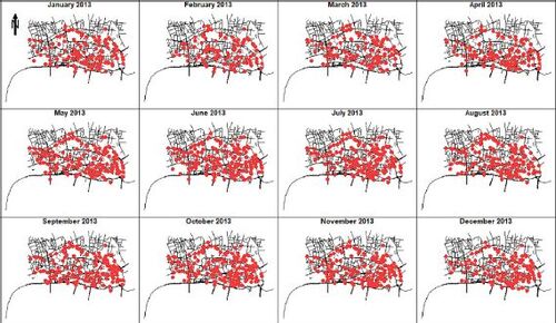
The street crime data contain 18,908 records for the study period including antisocial behavior, bicycle theft, drug-related, public disorder and weapons, public order, robbery, shoplifting, theft from the person, vehicle-related crime, violence and sexual offenses, and violent crime. Antisocial behavior comprises the maximum percentage of records (26.79%) followed by violence and sexual offenses (19.06%), and shoplifting (16.97%). Amongst all types of crimes, only antisocial behavior, shoplifting, vehicle-related, and drug-related crimes appeared in all months. Regarding the traffic accident data, it contains 1678 observations all being fatal accidents having at least one causality count. We note that most accidents (90.58%) are having only one causality. As showcases, the locations of traffic accidents and street crimes for the year 2013 are shown in Figures 1 and 2.

Figure 1. Monthly spatial point patterns of fatal traffic accidents in the city of London, UK, during 2013.

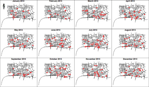
Figure 2. Monthly spatial point patterns of street crimes in the city of London, UK, during 2013.

We note that the road network is accessed from open street map (OSM) repository using the R package osmdata (Padgham et al. 2017). OSM data is free and licensed under the open data commons open database license (ODbL) by the OpenStreetMap Foundation (OSMF)¹. Initially, complete OSM street network for the entire study area has been retrieved using primary tag highway (used for any category of streets). Then, less important OSM highway categories such as unclassified, bus guideway, path, raceway, escape, and bridleway are not included in the current study. In fact, these categorizes are not used for usual traffic, and thus they do not host any event. Both data retrieval and cleaning has been performed using the same R package osmdata.

The traffic accident dataset is published by the Department of Transports, government of UK, under the UK government open data project². The street crime data is provided by 43 geographic police forces in the UK and Wales, the British Transport Police, the Police Service of Northern Ireland and the Ministry of Justice, and the government of UK. Both the traffic accidents and street crimes datasets are free and licensed under the Open Government License v3.0 for public sector information, government of UK³.

3. Point processes on linear networks

Throughout the article, we consider X as a simple spatial point process on the linear network $L\subset {\mathbb{R}}^2,$ which is a union of some finite number of segments $l_i=[u_i,v_i]=\{t{u}_i+(1-t)v_i:0\le t\le 1\}\subset {\mathbb{R}}^2,1\le i<\infty .$ We do not set any restriction regarding the connectivity of the network or the kind of intersection between different segments. The distance between any two points $u,v\in L$ is denoted by $d_L(u,v).$ For any subnetwork $A\subset L,$ its total length is obtained by summing the length of all its corresponding segments and is denoted by $\left|A\right|.$ For any measurable function $f:L\to [0,\infty ),$ the Campbell formula states that: $$\mathbb{E}\sum _{x\in X}f\left(x\right)={\int }_{L}f\left(u\right)\lambda \left(u\right)d_{1}u,$$ where $\lambda (·)$ is called the intensity function of X governing its distribution over L, and $d_1$ stands for integration with respect to arc length. In particular, $$\mathbb{E}\left[\#\left(A\cap X\right)\right]={\int }_A\lambda \left(u\right)d_{1}u,\hspace{1em}A\subset L,$$ where $\#(A\cap X)$ denotes the number of points of X falling in A. If $\lambda (u)\equiv \lambda ,$ then X is called a homogeneous point process, otherwise it is said to be an inhomogeneous point process (Ang, Baddeley, and Nair 2012; Baddeley, Rubak, and Turner 2015).

Due to the geometrical complexities of linear networks, estimating the intensity function $\lambda (·)$ has been quite challenging. Nevertheless, several proposals have been developed including some network-distance kernel-based smoothing methods (Okabe, Satoh, and Sugihara 2009; McSwiggan, Baddeley, and Nair 2016; Moradi, 2018; Moradi, Rodriguez-Cortes, and Mateu 2018), the two-dimensional convolution-based kernel intensity estimators (Rakshit et al. 2019), and the resample-smoothed Voronoi intensity estimator (Moradi et al. 2019). Consider $\mathbf{x}=\{x_1,x_2,\dots ,x_n\}$ as a realization of point process X on L, the two-dimensional convolution-based kernel intensity estimator, with uniform corrections, is of the form: (1) $${\widehat{\lambda }}^{\mathrm{U}}(u)=\frac{1}{c_L(u)}\sum _{i=1}^n\kappa (u-x_i),\mathrm{\hspace{1em}}\mathrm{\hspace{1em}}u\in L,$$(1) and with Jones-Diggle correction, it is given as (2) $${\widehat{\lambda }}^{\text{JD}}(u)=\sum _{i=1}^n\frac{1}{c_L(x_i)}\kappa (u-x_i),\mathrm{\hspace{1em}}\mathrm{\hspace{1em}}u\in L,$$(2) where κ is a bivariate kernel function, and $$c_L(u)={\int }_L\kappa (u-v){\mathrm{d}}_{1}v,$$ is an edge correction. The Eq. (1)(1) $${\widehat{\lambda }}^{\mathrm{U}}(u)=\frac{1}{c_L(u)}\sum _{i=1}^n\kappa (u-x_i),\mathrm{\hspace{1em}}\mathrm{\hspace{1em}}u\in L,$$(1) is unbiased if the true intensity $\lambda (·)$ is constant, and the Eq. (2)(2) $${\widehat{\lambda }}^{\text{JD}}(u)=\sum _{i=1}^n\frac{1}{c_L(x_i)}\kappa (u-x_i),\mathrm{\hspace{1em}}\mathrm{\hspace{1em}}u\in L,$$(2) provides mass conservation, i.e. ${\int }_L{\widehat{\lambda }}^{\text{JD}}(u){\mathrm{d}}_{1}u=n.$ For further details regarding different statistical properties of the Eqs. (1)(1) $${\widehat{\lambda }}^{\mathrm{U}}(u)=\frac{1}{c_L(u)}\sum _{i=1}^n\kappa (u-x_i),\mathrm{\hspace{1em}}\mathrm{\hspace{1em}}u\in L,$$(1) and (2)(2) $${\widehat{\lambda }}^{\text{JD}}(u)=\sum _{i=1}^n\frac{1}{c_L(x_i)}\kappa (u-x_i),\mathrm{\hspace{1em}}\mathrm{\hspace{1em}}u\in L,$$(2) , and additional details of relative risk see Rakshit et al. (2019).

It is common practice to estimate the spatially-varying relative frequency of each type of events, when there are several types of events occurring on the same network. Assume that two realizations $\mathbf{x}$ and $\mathbf{y}$ are observed, on the same network L, from two different point processes X and Y. The relative risk between the two types is then calculated by $\rho (u)=\mathit{log}({\lambda }_X(u)/{\lambda }_Y(u)),u\in L,$ in which ${\lambda }_X(·)$ and ${\lambda }_Y(·)$ stand for the intensity functions of X and Y, respectively. The literature recommends to estimate both ${\lambda }_X(·)$ and ${\lambda }_Y(·)$ using a common bandwidth (Kelsall and Diggle 1995; Hazelton 2008; Davies, Jones, and Hazelton 2016). Relative risk for point patterns on linear networks is substantially discussed by Rakshit et al. (2019) and McSwiggan, Baddeley, and Nair (2020).

4. Mann–Kendall trend detection

When dealing with observations that appear as ordered in time, a very first thing that might be of interest is to check whether, in the distribution of data, there is any gradual/sudden departure from its past norm. The importance of being aware of such departure, e.g. in model fitting and prediction, has led to the development of several proposals under different settings. Amongst all, the Mann–Kendall trend test has been one of the most frequently used trend tests in the literature (Mann 1945; Kendall 1948; Militino, Moradi, and Ugarte 2020). Generally, for trend detection methods, the null hypothesis ${\mathcal{H}}_0$ is that data is independently and randomly ordered, whereas the alternative hypothesis ${\mathcal{H}}_1$ claims the existence of a monotonic trend. In other words, the null hypothesis stands with no gradual change in data over time. Considering $\mathbf{y}=\{y_1,y_2,\dots ,y_m\},1<m<\infty ,$ as a finite set of numerical time-ordered observations, the test statistic of the univariate Mann–Kendall is given as (3) $$S=\sum _{i=1}^{m-1}\sum _{j=i+1}^m\text{sgn}\{y_j-y_i\},$$(3) where $$\text{sgn}\{y_j-y_i\}=\{\begin{array}{cc}1,\hfill & y_j-y_i>0,\hfill \\ 0,\hfill & y_j-y_i=0,\hfill \\ -1,\hfill & y_j-y_i<0.\hfill \end{array}$$

Under the null hypothesis, the expectation and variance of Eq. (3)(3) $$S=\sum _{i=1}^{m-1}\sum _{j=i+1}^m\text{sgn}\{y_j-y_i\},$$(3) are $\mathbb{E}\left[S\right]=0$ and $\text{Var}\left[S\right]=m(m-1)(2m+5)/18$ subject to there being no ties. The test statistic Eq. (3)(3) $$S=\sum _{i=1}^{m-1}\sum _{j=i+1}^m\text{sgn}\{y_j-y_i\},$$(3) compares each data point to all data appeared at a later time, looking for any gradual growth/shrinking in the data. Moreover, the so-called (rank correlation) Kendall’s τ is in close relation with Eq. (3)(3) $$S=\sum _{i=1}^{m-1}\sum _{j=i+1}^m\text{sgn}\{y_j-y_i\},$$(3) , being calculated as $S/\left(\begin{array}{c}m\\ 2\end{array}\right)$ if there is no tie in $\mathbf{y}.$ Note that positive/negative values of S are used as indicators of upward/downward trend in $\mathbf{y}.$ In practice, however, the standardized test statistic $Z=\left[\text{sgn}\right\{S\left\}\right(\left|S\right|-1\left)\right]/\sqrt{\text{Var}\left[S\right]}$ and its corresponding approximate p value (4) $$p=2\min (0.5,P(X>\left|Z\right|\left)\right),\hspace{1em}X\sim N(0,1),$$(4) are used to whether accept or reject the null hypothesis ${\mathcal{H}}_0.$ In addition, a multivariate version of the Mann–Kendall test is available for trend detection in a group of time-ordered datasets jointly. This takes information from all individual ones, combines the information and provides a corrected statistics based on the corresponding variance-covariance matrix (Libiseller and Grimvall 2002), and makes decision about the existence of trend in data without pointing to where dominance occurs in case a trend is detected (Pohlert 2018). Looking at the literature, the performance reduction of Mann–Kendall test in the presence of temporal autocorrelation has been frequently highlighted, suffering from a high rate of false positives. The higher the degree of autocorrelation, the higher the type I error probability (Yue et al. 2002). In order to remedy such an issue, several modifications have been developed including pre-whitening techniques (Kulkarni and von Storch 1995; Von Storch 1999; Yue et al. 2002; Hamed, 2009) and variance correction approaches (Hamed and Rao 1998; Yue and Wang 2004). Although these modifications generally reduce/moderate the type I error probability of the Mann–Kendall test, they inevitably decrease the power of the test which means increasing the type II error probability. However, in hypothesis testing a balance between the type I and type II error probabilities is needed. Under different settings, and through a comprehensive simulation study, it is shown that looking for a tradeoff between the type I error probability and the power of the test leads to the original Mann–Kendall test as a reliable and preferable test when data have experienced a monotonic trend (Militino, Moradi, and Ugarte 2020).

5. Results

This section is devoted to present the results of trend detection, based on the multivariate/univariate Mann–Kendall test, for the time series of estimated intensity images of fatal traffic accidents and street crimes in the city of London, UK, from January 2013 to December 2017, and also their corresponding time series of relative risk images. Prior to employ the Mann–Kendall test, we need to estimate the intensities and relative risk images. Since we are interested in the temporal evolution in the time series of estimated intensities of time-ordered spatial point patterns, and also to avoid undesirable halo artifacts, we make use of a common bandwidth for each time series of point patterns. Hence, for each such time series, we first select the bandwidth parameter using the Scott’s rule-of-thumb (Rakshit et al. 2019) for individual point patterns, and then use the geometrical mean of such selected bandwidths as a common choice. In the calculation of relative risk images we use the method of Davies (2013) to employ equal bandwidths for both the numerator and denominator for each individual risk, and again we make use of the geometrical mean of the selected bandwidths as a common choice in this case.

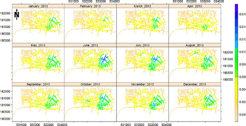
Each time series of point patterns contain 60 monthly patterns for which the common selected bandwidths for accidents data and street crime data are 277.19 and 179.12 m, respectively. The considered common bandwidth for relative risk calculation is 215.95 m. Figures 3 and 4 show the monthly estimated intensities, using the uniform edge correction, of fatal traffic accidents and street crimes in the city of London, UK, in 2013 respectively. Clearly, the estimated intensities in both cases vary across time, implying a change in the corresponding time of hot-spots and pointing to some spatial variation in the intensities. This indeed might be a sign of first-order non-separability. We did not overlay the network for a better visualization of spatial/temporal changes in the intensity images.

Figure 3. Monthly estimated intensities of the fatal traffic accident data in the city of London, UK, in 2013.

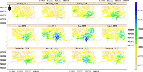
Figure 4. Monthly estimated intensities of the street crime data in the city of London, UK, in 2013.

Before turning to the trend detection problem, we note that for each pixel in Figures 3 and 4, or their corresponding relative risks, there exists a time series of estimated values. We are now interested in trend detection in such time series. Thus, we first deseason the data by creating seasonal anomalies of data (Appelhans, Detsch, and Nauss 2015), and then aggregate it with factor 2. Note that aggregation might reduce the number of potential false positives by smoothing out the estimated intensity images locally.

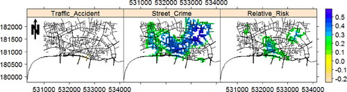
In order to study the existence of potential trend/change in the time series of estimated intensities and their corresponding relative risk more precisely, we next call the Mann–Kendall trend detection method. Nevertheless, being aware of the effect of temporal autocorrelation in the performance of trend/change-point detection methods, we initially calculate the first lag partial autocorrelation for the (pixel) time series of estimated intensities and relative risk images by fitting autoregressive models to each (pixel) time series of such values. Figure 5 shows how the first lag partial autocorrelation of such time series of images vary over the region. Amongst all, the time series of estimated intensities of street crimes show the highest temporal autocorrelation reaching its maximum in the center and eastern part of the network. The time series of estimated intensities of traffic accidents and relative risk generally show a low degree of temporal autocorrelation having their maximum around the central part of the region. Moreover, their spatial variation does not necessarily follow the same distribution, e.g. a location with high temporal autocorrelation in the time series of the estimated intensities of street crime does not necessarily show a high temporal autocorrelation in the time series of the estimated intensities of fatal traffic accidents. Looking back into the literature, areas with quite high temporal autocorrelation are vulnerable to introduce false positives in terms of trend/change-point detection (Serinaldi and Kilsby 2016; Militino, Moradi, and Ugarte 2020).

Figure 5. First lag partial autocorrelation for the time series of monthly estimated intensity and relative risk images of fatal traffic accident and street crime in the city of London, UK, in the period of January 2013 to December 2017.

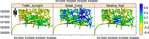
Turning to the trend detection problem, we first make use of the multivariate version of the Mann–Kendall method (Pohlert 2018) to check if there is any major area showing any significant monotonic trend that could dominate the behavior of data in question in the rest of the network. The obtained p values of multivariate Mann–Kendall for the corresponding time series of fatal traffic accident, street crime, and relative risk are 0.95, 3.7 × 10^–6, and 0.007, respectively. Therefore, the time series of estimated intensities of traffic accident data does not show any evidence of trend. Regarding the street crime data, there is a strong claim on the existence of a monotonic trend, and the time series of the estimated relative risk images also show a monotonic trend. Nevertheless, and in order to get an insight into where dominance occurs, we next employ the univariate Mann–Kendall method. Figure 6 shows the detected segments/pixels/locations in the network of the city of London, where the time series of the monthly estimated intensities of fatal traffic accidents, street crimes, and their corresponding relative risk show a monotonic trend in the period of January 2013 to December 2017. Apparently, the fatal traffic accident data does not show a particular trend in the network, apart from a very small area in the center of the southernmost street that shows a downward trend. The street crime dataset, however, generally shows an upward trend in many of the western, central, and northeastern streets. The time series of relative risk images shows three major areas with upward trend, in the (southern) center, northwest, and northeast of the network.

Figure 6. Detected pixels with significant trend based on the univariate Mann–Kendall test, at significance level 0.05, for the time series of monthly estimated intensity and relative risk images of fatal traffic accident and street crime in the city of London, UK, in the period of January 2013 to December 2017. Values represent the Kendall’s τ.

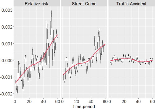
Looking into Figures 5 and 6 simultaneously, it is seen that detected areas with significant trend in Figure 6 somehow show a higher temporal autocorrelation than the rest of the network. Having this said, and being conscious of the adverse effect of temporal autocorrelation on the performance of Mann–Kendall method (Yue et al. 2002), we next aim at checking the behavior of individual pixel time series in the detected areas in Figure 6. However, since all detected pixels with significant trend, per each type in Figure 6, generally show similar trend, we look into their average behavior over time. Figure 7 shows the average time series of the detected pixels in Figure 6 in combination with their locally weighted smooth regression lines (Cleveland, Grosse, and Shyu 2017). The monotonic trend in the behavior of time series of the estimated intensities of street crime, and of the estimated relative risk of street crime with respect to traffic accident is clearly visible in Figure 7. Concerning the time series of the estimated intensities of traffic accidents, apparently there is a low slope downward trend from the middle of time series onwards.

Figure 7. Average relative risk and estimated intensities, after aggregation and deseasoning, of the detected significant pixels by the Mann–Kendall method, at significance level 0.05, together with their locally weighted smooth regression lines.

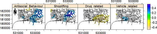
In addition, we next look for trend in the monthly estimated intensity images for different types of street crime such as antisocial behavior, shoplifting, vehicle-related, and drug-related crimes individually. Note these are the only types of street crimes appeared in all months. Figures 8 and 9 show their corresponding first lag partial autocorrelation and detected pixels with significant trend, respectively. It is clearly seen that these types of crimes show different behavior over the network. Further, from Figure 9 we can see that the estimated intensity of drug-related crimes has experienced a reduction over time in a big part of the network. Regarding other types of crimes, there are both upward and downward detected trends in different areas, where the major areas having upward trend belong to antisocial behavior and shoplifting, respectively. We add that the multivariate Mann–Kendall tests also gave rise to p values 0.05, 0.01, 9.1 × 10^–5, and 0.55 for anticocial behavior, shoplifting, drug-related, and vehicle-related crimes, respectively.

Figure 8. First lag partial autocorrelation for the time series of monthly estimated intensity images of different types of street crime in the city of London, UK, in the period of January 2013 to December 2017.

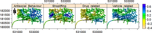
Figure 9. Detected pixels with significant trend based on the univariate Mann–Kendall test, at significance level 0.05, for the time series of monthly estimated intensity images of different types of street crime in the city of London, UK, in the period of January 2013 to December 2017.

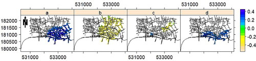
We further check the existence of any monotonic trend in the time-ordered relative risk images of different types of crimes with respect to each other. The multivariate Mann–Kendall test gave rise to p values 0.03 (antisocial behavior vs. drug-related), 3.35 × 10^–5 (drug-related vs. shoplifting), 0.43 (vehicle-related vs shoplifting), and 0.13 (vehicle-related vs. drug-related). We now employ the univariate Mann–Kendall test over each pixel time series to disclose the pixels/locations with trends. Figure 10 shows the locations where such relative risk time series have experienced monotonic trends. We have seen that the relative risk of antisocial behavior crimes with respect to drug-related crimes shows an increasing trend in the southeast of the network. The majority of the eastern part of the network shows a decreasing trend for the relative risk of drug-related crimes with respect to shoplifting. Also, the relative risk of vehicle-related crimes versus shoplifting shows a decreasing trend in a small area in the northeast of the network, together with an increasing trend in a few pixels in the south. Finally, the relative risk of vehicle-related versus drug-related crimes shows an increasing trend in most of the southern part of the network. These outputs show that the temporal changes in the relative risks between different types of crimes clearly varies over the network, there is no overall unique behavior, and moreover the slop of the trend varies among different risks. We did not find any significant trend for the relative risks between other combinations of crimes. We also add the first lag partial autocorrelation for the corresponding time series of the images displayed in Figure 10, in the detected pixels, is generally quite low with averages $0.03,0.21,0.28,$ and 0.08 for relative risks of antisocial behavior versus drug-related, drug-related versus shoplifting, vehicle-related against shoplifting, and vehicle-related against drug-related, respectively.

Figure 10. Detected pixels with significant trend based on the univariate Mann–Kendall test, at significance level 0.05, for the time series of monthly estimated relative risk images for antisocial vs. drug-related (a), drug-related vs. shoplifting (b), vehicle-related vs. shoplifting (c), and vehicle-related vs. drug-related (d) in the city of London, UK, in the period of January 2013 to December 2017.

6. Summary

On the one hand, the problem of trend detection in time series has been often called within different fields such as remote sensing, agronomy, finance, etc, due to its important role in model fitting and prediction. On the other hand, spatial point patterns may also appear as a time series of realizations. However, the field of point processes has not yet benefited from trend detection methods. In this article, we have combined the well-known trend detection problem with the recently gained attention topic of spatial point processes on linear networks. We have focused on the time series of monthly estimated intensities and relative risk images of fatal traffic accident and street crime in the city of London, UK, from January 2013 to December 2017. We have obtained the intensity and relative risk images by using the non-parametric kernel-based estimator of Rakshit et al. (2019). In our results, the time series of estimated intensities has shown that, for both datasets, they go under significant changes temporally and spatially which is a sign of first-order non-separability (an assumption which is commonly considered when analyzing spatio-temporal point patterns). The time series of estimated intensity images of traffic accident data has not generally shown a strong evidence of trend anywhere in the network. Conversely, the time series of estimated intensity images of street crime, and consequently its relative risk with respect to fatal traffic accident, however, have notably experienced a strong upward trend in mostly western, central, and northeastern parts of the network. Further, we have seen that different types of crimes show different behavior over the network, and consequently different behavior in terms of upward/downward trend. Generally, we have observed that the temporal changes in the intensity/relative risk images clearly varies over the network, and there is no overall unique behavior. Furthermore, the relative risks between certain types of crimes experience different types of trends over different regions in the city of London. Although the average time series of the locations with significant monotonic trend show evidence of such detected trend, distinguishing true and false positives needs further detailed research.

Regarding the limitations and future works, we note that one may estimate the intensities by means of parametric estimation to also reveal the effect of the characteristics of network over intensities/relative-risks such as distances to crossings, roundabouts, etc. Trend detection based on parametric intensity/relative-risk estimation may not necessarily lead to similar results. In addition, one may aim to model the time-ordered non-parametrically estimated intensities/relative-risks values based on some given/collected covariates to disclose their effect over the evolution of intensities/relative-risks over time. Such parametric modeling can further reveal what actually causes the trend. Moreover, another relevant and interesting idea might be to investigate the influence of autocorrelation, and also to detect the time index when trend starts to grow using e.g. deep-learning-based methods such as Long-short term memory (LSTM), Recurrent Neural Networks (RNN), and Convolutional Neural Network (CNN).

Our data and R codes, to reproduce the results, are available at https://github.com/Moradii/trend_intensity_images. Moreover, throughout the article, we have made use of the R packages stats (R Core Team 2020), spatstat (Baddeley and Turner 2005; Baddeley, Rubak, and Turner 2015), sparr (Davies, Marshall, and Hazelton 2018), remote (Appelhans, Detsch, and Nauss 2015), raster (Hijmans 2019), trend (Pohlert 2018), gimms (Detsch 2018), sp (Pebesma and Bivand 2005; Bivand, Pebesma, and Gomez-Rubio 2013), and ggplot2 (Wickham 2016).

Acknowledgments

The authors are grateful to the editor and three referees for constructive comments.

Additional information

Funding

Jorge Mateu has been partially funded by grants UJI-B2018-04 from Universitat Jaume I of Castellón (Spain), AICO/2019/198 from Generalitat Valenciana, and MTM2016-78917-R from Ministry of Science. Somnath Chaudhuri has been funded through the Erasmus Mundus programme by the European Commission under the Framework Partnership Agreement, FPA-2016-2054.

Notes

1 https://www.openstreetmap.org/copyright

2 https://data.gov.uk

3 http://www.nationalarchives.gov.uk/doc/open-government-license/version/3

References

- Ang, Q. W., A. Baddeley, and G. Nair. 2012. Geometrically corrected second order analysis of events on a linear network, with applications to ecology and criminology. Scandinavian Journal of Statistics 39 (4):591–617. doi:10.1111/j.1467-9469.2011.00752.x.
- Appelhans, T., F. Detsch, and T. Nauss. 2015. remote: Empirical orthogonal teleconnections in R. Journal of Statistical Software 65 (10):1–19. doi:10.18637/jss.v065.i10.
- Baddeley, A., E. Rubak, and R. Turner. 2015. Spatial point patterns: Methodology and applications with R. London: Chapman and Hall/CRC.
- Baddeley, A., and R. Turner. 2005. spatstat: An R package for analyzing spatial point patterns. Journal of Statistical Software 12 (6):1–42. doi:10.18637/jss.v012.i06.
- Bivand, R., E. Pebesma, and V. Gomez-Rubio. 2013. Applied spatial data analysis with R. 2nd ed. NY: Springer.
- Bullock, E. L., C. E. Woodcock, and C. E. Holden. 2020. Improved change monitoring using an ensemble of time series algorithms. Remote Sensing of Environment 238:111165. doi:10.1016/j.rse.2019.04.018.
- Cleveland, W. S., E. Grosse, and W. M. Shyu. 1992. Local regression models. Chapter 8 of Statistical models in S, eds. J. M. Chambers and T. J. Hastie, 309–76. Wadsworth & Brooks/Cole.
- Cox, D. R., and A. Stuart. 1955. Some quick sign tests for trend in location and dispersion. Biometrika 42 (1-2):80–95. doi:10.1093/biomet/42.1-2.80.
- Davies, T. M. 2013. Jointly optimal bandwidth selection for the planar kernel-smoothed density-ratio. Spatial and Spatio-Temporal Epidemiology 5:51–65. doi:10.1016/j.sste.2013.04.001.
- Davies, T. M., K. Jones, and M. L. Hazelton. 2016. Symmetric adaptive smoothing regimens for estimation of the spatial relative risk function. Computational Statistics & Data Analysis 101:12–28. doi:10.1016/j.csda.2016.02.008.
- Davies, T. M., J. C. Marshall, and M. L. Hazelton. 2018. Tutorial on kernel estimation of continuous spatial and spatiotemporal relative risk. Statistics in Medicine 37 (7):1191–221. doi:10.1002/sim.7577.
- Detsch, F. 2018. gimms: Download and process GIMMS NDVI3g data. R package version 1.1.1.
- Feng, S., Z. Li, Y. Ci, and G. Zhang. 2016. Risk factors affecting fatal bus accident severity: Their impact on different types of bus drivers. Accident; Analysis and Prevention 86:29–39. doi:10.1016/j.aap.2015.09.025.
- Grundy, T., R. Killick, and G. Mihaylov. 2020. High-dimensional changepoint detection via a geometrically inspired mapping. Statistics and Computing 30 (4):1155–66. doi:10.1007/s11222-020-09940-y.
- Hamed, K. 2009. Enhancing the effectiveness of prewhitening in trend analysis of hydrologic data. Journal of Hydrology 368 (1-4):143–55. doi:10.1016/j.jhydrol.2009.01.040.
- Hamed, K., and A. R. Rao. 1998. A modified Mann–Kendall trend test for autocorrelated data. Journal of Hydrology 204 (1-4):182–96. doi:10.1016/S0022-1694(97)00125-X.
- Hazelton, M. L. 2008. Kernel estimation of risk surfaces without the need for edge correction. Statistics in Medicine 27 (12):2269–72. doi:10.1002/sim.3047.
- Hijmans, R. J. 2019. raster: Geographic data analysis and modeling. R Package Version 2.8–19.
- Hipp, J. R., Y. A. Kim, and K. Kane. 2019. The effect of the physical environment on crime rates: Capturing housing age and housing type at varying spatial scales. Crime & Delinquency 65 (11):1570–95. doi:10.1177/0011128718779569.
- Kelsall, J. E., and P. Diggle. 1995. Kernel estimation of relative risk. Bernoulli 1 (1/2):3–16. doi:10.2307/3318678.
- Kendall, M. G. 1948. Rank correlation methods. Oxford, England: Griffin.
- Kulkarni, A., and H. von Storch. 1995. Monte carlo experiments on the effect of serial correlation on the Mann–Kendall test of trend. Meteorologische Zeitschrift 4 (2):82–85. doi:10.1127/metz/4/1992/82.
- Libiseller, C., and A. Grimvall. 2002. Performance of partial mann–kendall tests for trend detection in the presence of covariates. Environmetrics 13 (1):71–84. doi:10.1002/env.507.
- Mann, H. B. 1945. Nonparametric tests against trend. Econometrica 13 (3):245–59. doi:10.2307/1907187.
- Matteson, D. S., and N. A. James. 2014. A nonparametric approach for multiple change point analysis of multivariate data. Journal of the American Statistical Association 109 (505):334–45. doi:10.1080/01621459.2013.849605.
- McSwiggan, G., A. Baddeley, and G. Nair. 2016. Kernel density estimation on a linear network. Scandinavian Journal of Statistics 44 (2):324–45. doi:10.1111/sjos.12255.
- McSwiggan, G., A. Baddeley, and G. Nair. 2020. Estimation of relative risk for events on a linear network. Statistics and Computing 30 (2):469–84. doi:10.1007/s11222-019-09889-7.
- Militino, A. F., M. Moradi, and M. D. Ugarte. 2020. On the performance of trend and change-point detection methods for remote sensing data. Remote Sensing 12 (6):1008. doi:10.3390/rs12061008.
- Moradi, M. 2018. Spatial and spatio-temporal point patterns on linear networks. PhD diss., University Jaume I.
- Moradi, M.,. O. Cronie, E. Rubak, R. Lachieze-Rey, J. Mateu, and A. Baddeley. 2019. Resample-smoothing of Voronoi intensity estimators. Statistics and Computing 29 (5):995–1010. doi:10.1007/s11222-018-09850-0.
- Moradi, M.,. F. Rodriguez-Cortes, and J. Mateu. 2018. On kernel-based intensity estimation of spatial point patterns on linear networks. Journal of Computational and Graphical Statistics 27 (2):302–11. doi:10.1080/10618600.2017.1360782.
- Okabe, A., T. Satoh, and K. Sugihara. 2009. A kernel density estimation method for networks, its computational method and a GIS-based tool. International Journal of Geographical Information Science 23 (1):7–32. doi:10.1080/13658810802475491.
- Padgham, M., B. Rudis, R. Lovelace, and M. Salmon. 2017. osmdata. The Journal of Open Source Software 2 (14):305. doi:10.21105/joss.00305.
- Pebesma, E., and R. Bivand. 2005. Classes and methods for spatial data in R. R News 5 (2):9–13.
- Pettitt, A. N. 1979. A non-parametric approach to the change-point problem. Journal of the Royal Statistical Society: Series C (Applied Statistics) 28 (2):126–35. doi:10.2307/2346729.
- Pohlert, T. 2018. trend: Non-parametric trend tests and change-point detection. R package version 1.1.1.
- Rakshit, S., T. M. Davies, M. Moradi, G. McSwiggan, G. Nair, J. Mateu, and A. Baddeley. 2019. Fast kernel smoothing of point patterns on a large network using two-dimensional convolution. International Statistical Review 87 (3):531–56. doi:10.1111/insr.12327.
- R Core Team. 2020. R: A Language and Environment for Statistical Computing. Vienna, Austria: R Foundation for Statistical Computing.
- Serinaldi, F., and C. G. Kilsby. 2016. The importance of prewhitening in change point analysis under persistence. Stochastic Environmental Research and Risk Assessment 30 (2):763–77. doi:10.1007/s00477-015-1041-5.
- Truong, C., L. Oudre, and N. Vayatis. 2020. Selective review of offline change point detection methods. Signal Processing 167:107299. doi:10.1016/j.sigpro.2019.107299.
- Verbesselt, J., R. Hyndman, G. Newnham, and D. Culvenor. 2010. Detecting trend and seasonal changes in satellite image time series. Remote Sensing of Environment 114 (1):106–15. doi:10.1016/j.rse.2009.08.014.
- Von Storch, H. 1995. Misuses of statistical analysis in climate research. In Analysis of Climate Variability: Applications of Statistical Techniques, ed. H. von Storch and A. Navara, 11–26. Berlin, Germany: Springer-Verlag.
- Wickham, H. 2016. ggplot2: Elegant graphics for data analysis. New York: Springer-Verlag.
- Yamada, I., and J. C. Thill. 2004. Comparison of planar and network K-functions in traffic accident analysis. Journal of Transport Geography 12 (2):149–58. doi:10.1016/j.jtrangeo.2003.10.006.
- Yue, S., P. Pilon, B. Phinney, and G. Cavadias. 2002. The influence of autocorrelation on the ability to detect trend in hydrological series. Hydrological Processes 16 (9):1807–29. doi:10.1002/hyp.1095.
- Yue, S., and C. Wang. 2004. The mann-kendall test modified by effective sample size to detect trend in serially correlated hydrological series. Water Resources Management 18 (3):201–18. doi:10.1023/B:WARM.0000043140.61082.60.
- Zeileis, A., C. Kleiber, W. Krämer, and K. Hornik. 2003. Testing and dating of structural changes in practice. Computational Statistics & Data Analysis 44 (1-2):109–23. doi:10.1016/S0167-9473(03)00030-6.