Exponential dispersion models for overdispersed zero-inflated count data

Abstract

We consider two classes of exponential dispersion models of discrete probability distributions which are defined by specifying their variance functions in their mean value parameterization. These classes were considered in our earlier paper as models of overdispersed zero-inflated distributions. In this paper we analyze the application of these classes to fit count data having overdispersed and zero-inflated statistics. For this reason, we first elaborate on the computational aspects of the probability distributions, before we consider the data fitting with our models. We execute an extensive comparison with other statistical models that are recently proposed, on both real data sets, and simulated data sets. Our findings are that our framework is a flexible tool that gives excellent results in a wide range of cases. Moreover, specifically when the data characteristics show also large skewness and kurtosis our models perform best.

Keywords:

• Count data analysis
• Exponential dispersion models
• Fit models
• Overdispersion
• Poisson-tweedie model
• Zero-inflation

1. Introduction

In many scientific fields, one deals with systems, experiments, or phenomena that have random discrete outcomes. These outcomes are revealed typically through a set of data obtained by observing the system and counting the occurrences. The next issue is to describe statistically the system, modeling the occurrences by a discrete random variable, or just by a discrete probability distribution. Indeed, this is our starting point: we consider a number of sets of different count data, each from another application, and our goal is to fit suitable discrete distributions. In Bar-Lev and Ridder (2021) we have developed a framework of exponential dispersion models for count data, which resulted in two classes of parametric families of discrete distributions presented in terms of their variance functions. We proved that these two classes have some desirable properties. Each of these classes was shown to be overdispersed and zero inflated in ascending order, making them as competitive statistical models for those in use in statistical modeling.

The contribution of this paper is, firstly, that we elaborate on the computational aspects of these distributions, and secondly, that we use our framework for fitting data sets. We shall examine the goodness-of-fit of the proposed distributions when applied not only to real data sets, but also to simulated data sets that were generated to have certain statistical characteristics. Moreover, we shall compare our fits with known fits from literature. Specifically, we consider data that show (i) overdispersion, meaning the variance is greater than the mean; and (ii) zero-inflation, i.e. a high occurrence of zero values. We shall see that our framework allows for very flexible modeling in all kinds of different statistical situations. Finally, we show empirically that our models outperform specifically in the cases with large skewness and kurtosis.

1.1. Literature review

Modeling count data by parametric families of discrete distributions has always been part of the statistical literature. Traditional models of count data were based on the Poisson and the negative binomial distributions, for instance in case of

• actuarial sciences for car insurance claims (Gossiaux and Lemaire 1981), hospitalizations (Klugman, Panjer, and Willmot 1998), motor vehicle crashes (Lord, Washington, and Ivan 2005);

• health economics for kidneys cysts (Chan et al. 2010), Thalassemia disease among children (Zafakali and Ahmad 2013), bovine tuberculosis cases (Coly et al. 2016);

• psychology and behavioral sciences for cigarette smoking (Siddiqui et al. 1999), alcohol drinking (Armeli et al. 2005), prison incidents (Walters 2007).

The advantages of the Poisson and negative binomial distributions are their easy computations and parameter estimation. The main disadvantage of the Poisson distribution is its variance being equal to its mean. Thus, this distribution does not fit the data properly in case of overdispersion. The negative binomial distribution is an improvement since it can model overdispersion, however it could give poor fits to data with an excessive number of zeros (Coly et al. 2016).

In view of this, many other statistical models have been proposed and studied. An abundance of studies of new models can be observed in recent years, the reason being the availability of many diverse data sources, but more importantly, the advances in computational techniques. Commonly, the purpose is to handle overdispersion, or to handle zero-inflation; less frequently to handle both.

To name a few concerning handling overdispersion which are relevant for our study, generalized negative binomial (Jain and Consul 1971), Poisson-inverse Gaussian distribution (Willmot 1987), strict arcsine distribution (Kokonendji and Khoudar 2004), Poisson-Tweedie (Kokonendji, Dossou-Gbété, and Demétrio 2004), discrete Lindley distribution (Gomez-Deniz and Calderin-Ojeda 2011), a new logarithmic distribution (Gomez-Deniz, Sarabia, and Calderin-Ojeda 2011), discrete Gamma distribution (Chakraborty and Chakravarty 2012), and discrete generalized Rayleigh distribution (Alamatsaz et al. 2016). See Coly et al. (2016), for a review on other models and applications.

Concerning the development of models to handle zero-inflation, we mention zero-inflated Poisson (Lambert 1992), zero-inflated negative binomial (Ridout, Hinde, and Demétrio 2001), and a modeling based on copula functions (Zhao and Zhou 2012), and for a review on more models and applications we refer to Yip and Yau (2005). A few studies considered the development of models for both overdispersed and zero-inflated data, for instance, generalized Poisson (Consul 1989), and geometric discrete Pareto distribution (Bhati and Bakouch 2019), exponentiated discrete Lindley distribution (El-Morshedy, Eliwa, and Nagy 2020).

All above mentioned models deal with parametric distributions. The parameters are estimated directly from the data by moment matching or maximum likelihood estimation. Another statistical way of estimating the parameters of these distributions is by considering the concept of generalized linear models. For instance, Poisson regression is a generalized linear model with Poisson distribution error structure and the natural logarithm link function. We refer to Fahrmeir and Osuna Echavarría (2006) for an overview of regression models dealing with both overdispersed and zero-inflated data.

The approach that we followed for developing our fitted models is based on the concept of natural exponential families, and its generalization to exponential dispersion models (Bar-Lev and Kokonendji 2017; Jørgensen 1997). These models play an important role in probabilistic and statistical modeling. Many well-known distributions and families of distributions are included in these models. For instance, when considering counting distributions, the Poisson, negative binomial, genaralized Poisson, generalized negative binomial, and Poisson-inverse Gaussian distributions are special cases of exponential dispersion models. Moreover, they show nice mathematical properties which are convenient for the practical fitting of data. We defer theoretical details on natural exponential families, exponential dispersion models, and our usage of these models to Sec. 2. In Sec. 3 we will elaborate on the computation of the probabilities and show some descriptive properties. Sec. 4 concerns fitting our models to real data and to simulated data, and compare with seven models recently developed in the literature for the same purposes. The performance of a model is expressed by the loglikelihood value, the ${\chi }^2$ statistic and its p-value, the root mean square error (RMSE), and the Kullback-Leibler divergence . Based on the results, we discuss the suitability of our models, specifically in case the data show large skewness and kurtosis.

2. Families of probability distributions

In this section we first summarize the techniques of modeling probability distributions based on the concepts of natural exponential families, exponential dispersion models, and mean parameterization. For more details we refer to Bar-Lev and Kokonendji (2017); Jørgensen and Kokonendji (2016); Letac and Mora (1990). Also, we present our specific classes of these models.

2.1. Natural exponential families

Natural exponential families of distributions form a classic tool in statistical modeling and analysis, e.g. see Barndorff-Nielsen (1978). We give the definition here to introduce our notation. Let μ be a positive Radon measure on the Borel sets of the real line $\mathbb{R},$ with convex support, and define $\Theta \doteq \{\theta \in \mathbb{R}:\int e^{\theta x}\mu (dx)<\infty \},$ where we use the symbol $\doteq$ for “defined to be equal to”. Assume that Θ is nonempty and open. According to the Hölder’s inequality, Θ is an interval. We define for $\theta \in \Theta$ the cumulant transform $$\kappa (\theta )\doteq \hspace{0.17em}\text{log}\hspace{0.17em}\int e^{\theta x} \mu (dx).$$

Then, the natural exponential family $\mathcal{F},$ generated by μ is defined by the set of probability distributions (1) $$\mathcal{F}\doteq \{F_{\theta }:F_{\theta }(dx)\doteq e^{\theta x-\kappa (\theta )} \mu (dx):\theta \in \Theta \}.$$(1)

The measure μ is called the kernel of the family. The family is parameterized by the natural parameter θ. Differentiation is permitted and gives the mean $m(\theta )={\kappa }^{\prime }(\theta )$ and variance $V(\theta )={\kappa }^{″}(\theta ).$

2.2. Exponential dispersion models

The concept of natural exponential families generalizes in the following manner to exponential dispersion models which gives the statistical practitioner a convenient framework (Jørgensen 1997). Given a natural exponential family $\mathcal{F}$ with kernel μ and cumulant $\kappa (\theta ),$ let Λ be the set of p > 0 such that $p\kappa (\theta )$ is the cumulant transform for some measure μ_p. Thus for any $p\in \Lambda ,$ we get a natural exponential family of the form (2) $${\mathcal{F}}_p\doteq \{F_{(\theta ,p)}:F_{(\theta ,p)}(dx)\doteq e^{\theta x-p\kappa (\theta )} {\mu }_p(dx):\theta \in \Theta \}.$$(2)

This family of distributions, parameterized by pairs $(\theta ,p)\in \Theta \times \Lambda$ is called the exponential dispersion model. Parameter p is called the dispersion parameter. Many useful families of discrete distributions belong to exponential dispersion models (Kokonendji, Dossou-Gbété, and Demétrio 2004), and for this reason these models are important for fitting discrete data. Furthermore, exponential dispersion models show convenient properties, such as closure under convolution, and infinite divisibility (iff $\lambda =(0,\infty )$), see Jørgensen (1997) for more details.

2.3. Mean parameterization

For our purposes it is convenient to consider a reparameterization of the exponential dispersion model, similarly as has been introduced in Letac and Mora (1990) for natural exponential families. Starting point is the family of distributions defined in (2), in which we denote the cumulant by ${\kappa }_p(\theta )\doteq p\kappa (\theta ).$ Recall that any distribution $F_{(\theta ,p)}$ of the family has mean $m_p(\theta )={\kappa }_p^{\prime }(\theta ),$ and variance $V_p(\theta )={\kappa }_p^{\prime }(\theta ).$ The image of the differentiation of the cumulant, i.e. ${\mathcal{M}}_p\doteq {\kappa }_p^{\prime }(\Theta ),$ is called the mean domain of the family ${\mathcal{F}}_p.$ Because the map $\theta \mapsto {\kappa }_p^{\prime }(\theta )$ is one-to-one, its inverse function ${\psi }_p:{\mathcal{M}}_p\to \Theta$ is well defined, i.e. (3) $${\psi }_p(m)\doteq {({\kappa }_p^{\prime })}^{-1}(m),m\in {\mathcal{M}}_p.$$(3)

The corresponding variance function is $V_p(m)\doteq V_p({\psi }_p(m)).$ Furthermore, we define (4) $${\varphi }_p(m)\doteq {\kappa }_p({\psi }_p(m)),m\in {\mathcal{M}}_p.$$(4)

In this way the natural exponential family ${\mathcal{F}}_p$ is modeled by its mean parameterization, (5) $${\mathcal{F}}_p=\{F_{(m,p)}:F_{(m,p)}(dx)\doteq e^{{\psi }_p(m)x-{\varphi }_p(m)} {\mu }_p(dx):m\in {\mathcal{M}}_p\},p\in \Lambda .$$(5)

Note that the mean parameterization has an associated variance function $V_p(m)$ on the mean domain ${\mathcal{M}}_p.$ Conversely, when an exponential dispersion model ${\mathcal{F}}_p, p\in \Lambda$ is given by the pair $({\mathcal{M}}_p,V_p(m)),$ we find the distributions by (6) $${\psi }_p(m)=\int \frac{1}{V_p(m)} dm;\hspace{1em}{\varphi }_p(m)=\int \frac{m}{V_p(m)} dm.$$(6)

In our study we are interested in discrete distributions, say with probability mass functions $f(n)=\mathcal{P}(X=n),n=0,1,\dots ,$ where X represents the associated random variable. Specifically, we consider distributions belonging to exponential dispersion models, using the mean parameterization. Thus, the probability mass functions are represented by (7) $$f_{(m,p)}(n)\doteq {\mu }_p(n)e^{n{\psi }_p(m)-{\varphi }_p(m)},n=0,1,\dots .$$(7)

2.4. Variance function classes

Here we present the two models (or families) of distributions that were considered in Bar-Lev and Ridder (2021) as a means of a general framework for zero-inflated, overdispersed probability distributions. The models are defined through their variance function classes of the mean parameterization.

• ABM class, named after Awad, Bar-Lev, and Makov (2016), with mean m > 0, and variance function (8) $$V_p(m)=m{(1+\frac{m}{p})}^r, p>0,r=1,2,\dots .$$(8)

  Note that we exclude the r = 0 case, which would give the Poisson distribution. The case r = 1 gives the negative binomial distribution. The case r = 2 is called generalized Poisson (Consul 1989), or Abel distribution (Letac and Mora 1990).

• LM class with mean m > 0 and variance function (9) $$V_p(m)=\frac{m}{{(1-\frac{m}{p})}^r}, p>m,r=1,2,\dots .$$(9)

  Note that the mean domain of this class is a finite interval, ${\mathcal{M}}_p=(0,p).$ This class refers to Letac and Mora (1990), however, contrarily to the ABM class, the LM class belongs to a non-steep natural exponential family. Steepness of a natural exponential family is a property of its cumulant transform $\kappa (\theta )$ (Barndorff-Nielsen 1978).

It has been shown in Letac and Mora (1990) that the natural exponential families associated with these classes of variance functions are concentrated on the nonnegative integers. To our best knowledge these distributional models have not been used before in statistical fitting to real data, except for the trivial cases. We have considered in Bar-Lev and Ridder (2019) the Abel distribution for modeling insurance claim data.

It is easy to see that both two classes show overdispersion, $V_p(m)>m,$ and that the dispersion increases with the power r in the expressions (8)-(9) of the variance functions. Moreover, in Bar-Lev and Ridder (2021) we have shown that both classes satisfy also an increasing zero-inflation property. This means, denoting $f_{(m,p)}(0;r)$ for the probability mass in zero given mean m, dispersion parameter p and power r in the variance function, then $$f_{(m,p)}(0;r)<f_{(m,p)}(0;r+1),r=1,2,\dots .$$

These properties make the two classes a flexible tool for fitting overdispersed, zero-inflated data, which we will show in the sequel. For this purpose, however, we have to consider a method for computing the probability dsitributions.

2.5. Poisson-tweedie mixtures

Our two classes are two special exponential dispersion models in the sense that (i) they satisfy to be concentrated on the nonnegative integers, and (ii) their variance functions are exponential functions. Moreover, we consider the power parameter to be integer, which leads to a polynomial variance function (ABM), or a rational function (LM). Property (i) is a consequence of the sufficient and necessary conditions for variance functions that are established in Letac and Mora (1990). Other exponential dispersion models satisfying (i) and (ii) are the Hinde-Demétrio class with variance $V(m)=m+m^{\gamma }$ (Hinde and Demétrio 1998; Kokonendji, Dossou-Gbété, and Demétrio 2004), Poisson-Tweedie mixture class with variance $V(m)=m+p^{1-\gamma }{m}^{\gamma }$ (Jørgensen and Kokonendji 2016; Kokonendji, Dossou-Gbété, and Demétrio 2004), and Poisson-exponential-Tweedie models which have the variance function $V(m)=m+m^2+p^{1-\gamma }{m}^{\gamma }$ (Jørgensen and Kokonendji 2016), where exponent $\gamma >0$ may be non-integer. All these classes are based on mixing Poisson probabilities by a Tweedie distribution, which is inherently different from our approach. Also these classes are useful for overdispersed zero-inflated data as has been exposed in Jørgensen and Kokonendji (2016). In Sec. 4 of our data fitting analysis we shall include the Poisson-Tweedie mixture model.

3. Computing distributions

In this section we elaborate the numerical methods concerning computation of our distributions. The general procedure follows the guidelines of Letac and Mora (1990). Let be given a variance function V(m) of a natural exponential family of discrete distributions, where we have dropped the subscript dispersion parameter p for ease of notation and exposition. Recall the integral equations (6)(6) $${\psi }_p(m)=\int \frac{1}{V_p(m)} dm;\hspace{1em}{\varphi }_p(m)=\int \frac{m}{V_p(m)} dm.$$(6) .

1. We solve for primitives $\tilde{\psi }$ and $\tilde{\varphi }$ of the integral equations with zero constant of integration. All solutions are $$\psi (m)=\tilde{\psi }(m)+c_0;\varphi (m)=\tilde{\varphi }(m)+d_0,c_0,d_0\in \mathbb{R}.$$

   The specific constants c₀ and d₀ are obtained by the boundary conditions (10) $$\underset{m\to 0}{\lim }m e^{-\psi (m)}=1\hspace{1em}\text{and}\hspace{1em}\underset{m\to 0}{\lim }\varphi (m)=0.$$(10) Define (11) $$G(m)=m e^{-\psi (m)}.$$(11) The kernel ${(\mu (n))}_{n=0}^{\infty }$ is computed according to (12) $$\begin{array}{cc}\mu (0)& =e^{\varphi (0)}\\ \mu (n)& =\frac{1}{n!}{(\frac{d}{dm})}^{n-1}{e}^{\varphi (m)}{\varphi }^{\prime }(m){(G(m))}^n{|}_{m=0},\hspace{1em}n=1,2,\dots .\end{array}$$(12)

2. Note that the d₀ constant of the $\varphi$ function equals $$d_0=-\tilde{\varphi }(0).$$

   It is convenient to introduce $\tilde{\xi }$ and ξ functions, by (13) $$\tilde{\xi }(m)\doteq \tilde{\psi }(m)-\hspace{0.17em}\text{log}\hspace{0.17em}(m);\hspace{1em}\xi (m)\doteq \tilde{\xi }(m)+c_0=\psi (m)-\hspace{0.17em}\text{log}\hspace{0.17em}(m).$$(13) Then the c₀ constant of the ψ function equals $$c_0=-\tilde{\xi }(0),$$

and $G(m)=e^{-\xi (m)}.$

• 3. The main difficulty lies in computing the kernel as in (12). Define for $n=1,2,\dots$ $$F_n(m)\doteq e^{\varphi (m)} {\varphi }^{\prime }(m) {(G(m))}^n,$$

and $H_n(m)\doteq \hspace{0.17em}\text{log}\hspace{0.17em}{F}_n(m).$ Thus, $$H_n(m)=\varphi (m)+\hspace{0.17em}\text{log}\hspace{0.17em}{\varphi }^{\prime }(m)-n\xi (m).$$

It is easy to see that $$H_n(0)=\varphi (0)+\hspace{0.17em}\text{log}\hspace{0.17em}{\varphi }^{\prime }(0)-n\xi (0)=0+\hspace{0.17em}\text{log}\hspace{0.17em}1-n(\tilde{\xi }(0)+c_0)=0.$$ The next step is to compute the $(n-1)$-st derivative of $F_n(m)$ in (12). Apply the chain rule: $$\begin{array}{c}{(\frac{d}{dm})}^{n-1}{F}_n(m)={(\frac{d}{dm})}^{n-1}{e}^{H_n(m)}\\ =\sum \frac{(n-1)!}{k_1!k_2!\cdots k_{n-1}!} {\left({(\frac{d}{dx})}^k{e}^x\right)}_{x=H_n(m)} \prod _{j=1}^{n-1}(\frac{H_n^{(j)}(m)}{j!}{)}^{k_j},\end{array}$$

where the sum is over all nonnegative integer solutions of the Diophantine equation ${\sum }_{j=1}^{n-1}j{k}_j=n-1,$ and where $k={\sum }_{j=1}^{n-1}{k}_j.$ In the next sections we compute the derivatives $H_n^{(j)}(m)$ for the separate classes. The final computation for kernel $\mu (n)$ involves evaluating these expressions in m = 0, and dividing by $n!.$ Thus, (14) $$\begin{array}{c}\mu (n)=\frac{1}{n!}({(\frac{d}{dm})}^{n-1}{e}^{{\psi }_1(m)} {\psi }_1^{\prime }(m) {(G(m))}^n){|}_{m=0}\\ =\frac{1}{n!}\left({(\frac{d}{dm})}^{n-1}{e}^{H_n(m)}\right){|}_{m=0}\\ =\frac{1}{n!}\sum \frac{(n-1)!}{k_1!k_2!\cdots k_{n-1}!} {\left({(\frac{d}{dx})}^k{e}^x\right)}_{x=H_n(0)} \prod _{j=1}^{n-1}((\frac{H_n^{(j)}(m)}{j!}){|}_{m=0}{)}^{k_j}\\ =\frac{1}{n}\sum \frac{1}{k_1!k_2!\cdots k_{n-1}!} \prod _{j=1}^{n-1}(\frac{H_n^{(j)}(0)}{j!}{)}^{k_j}\\ =\frac{1}{n}\sum \prod _{j=1}^{n-1}\prod _{t=1}^{k_j}\frac{H_n^{(j)}(0)/j!}{t}.\end{array}$$(14)

3.1. Computing ABM distribution

Recall that the variance function is given by $$V(m)=m{(1+\frac{m}{p})}^r, r=2,3,\dots .$$

The integral equations are solved by (Bar-Lev and Ridder 2021) $$\begin{array}{l}\tilde{\psi }(m)=\hspace{0.17em}\text{log}\hspace{0.17em}(m)+\sum _{i=1}^{r-1}{c}_i {(m+p)}^{-i}+c_r\hspace{0.17em}\text{log}\hspace{0.17em}(m+p);\\ \tilde{\varphi }(m)=d_{r-1} {(m+p)}^{-r+1},\end{array}$$ where the coefficients $c_i,d_{r-1}$ are, $$\begin{array}{c}{c}_i=\{\begin{array}{cc}\frac{p^i}{i}& i=1,\dots ,r-1;\\ -1\hspace{1em}& i=r;\end{array}\hspace{1em}\\ d_{r-1}=-p^r/(r-1).\end{array}$$

Furthermore, $${\varphi }^{\prime }(m)=m/V(m)=p^r{(m+p)}^{-r}=\hspace{0.17em}\text{exp}\hspace{0.17em}(r\hspace{0.17em}\text{log}\hspace{0.17em}(p)-r\hspace{0.17em}\text{log}\hspace{0.17em}(m+p)).$$

We get $$\begin{array}{c}{H}_n(m)=\varphi (m)+\hspace{0.17em}\text{log}\hspace{0.17em}{\varphi }^{\prime }(m)-n\xi (m)\\ =d_{r-1}{(m+p)}^{-r+1}+d_0+r\hspace{0.17em}\text{log}\hspace{0.17em}(p)-r\hspace{0.17em}\text{log}\hspace{0.17em}(m+p)-n\sum _{i=1}^{r-1}{c}_i{(m+p)}^{-i}-n{c}_r\hspace{0.17em}\text{log}\hspace{0.17em}(m+p)-n{c}_0\\ =q_0+\sum _{i=1}^{r-1}{q}_i{(m+p)}^{-i}+q_r\hspace{0.17em}\text{log}\hspace{0.17em}(m+p),\end{array}$$ with $$\begin{array}{c}{q}_0=d_0+r\hspace{0.17em}\text{log}\hspace{0.17em}(p)-n{c}_0\\ q_i=-n{c}_i,i=1,\dots ,r-2\\ q_{r-1}=d_{r-1}-n{c}_{r-1}\\ q_r=-r-n{c}_r\end{array}$$

The j-th derivative of the $H_n(m)$ function becomes $$H_n^{(j)}(m)=\sum _{i=1}^{r-1}{q}_i{(\frac{d}{dm})}^j{(m+p)}^{-i}+q_r{(\frac{d}{dm})}^j\hspace{0.17em}\text{log}\hspace{0.17em}(m+p).$$

Thus, by defining $$h_n(i,j)=\{\begin{array}{cc}\frac{1}{j!}\left({(\frac{d}{dm})}^j{(m+p)}^{-i}\right){|}_{m=0}={(-1)}^j \left(\begin{array}{c}j+i-1\\ j\end{array}\right) p^{-i-j}\hfill & \hspace{1em}i=1,\dots ,r-1;\hfill \\ \frac{1}{j!}({(\frac{d}{dm})}^j\hspace{0.17em}\text{log}\hspace{0.17em}(m+p)){|}_{m=0}={(-1)}^{j-1} \frac{1}{j} p^{-j}\hfill & \hspace{1em}i=r,\hfill \end{array}$$ we obtain for the kernel $\mu (n)$ in (14), $$\mu (n)=\frac{1}{n}\sum \prod _{j=1}^{n-1}\prod _{t=1}^{k_j}\sum _{i=1}^r\frac{q_i{h}_n(i,j)}{t}.$$

3.2. Computing LM distribution

The variance function is $$V(m)=m{(1-\frac{m}{p})}^{-r}, r=1,2,\dots ,0<m<p.$$

The procedure is similar to computing the ABM and LMS distributions. Now it holds that (Bar-Lev and Ridder 2021) $$\begin{array}{c}\tilde{\psi }(m)=\hspace{0.17em}\text{log}\hspace{0.17em}(m)+\sum _{i=1}^r{c}_i m^i;\\ \tilde{\varphi }(m)=d_{r+1}{(p-m)}^{r+1},\end{array}$$ where $$\begin{array}{c}{c}_i={(-1)}^i\left(\begin{array}{c}r\\ i\end{array}\right)\frac{1}{i{p}^i}\hspace{1em}i=1,\dots ,r;\\ d_{r+1}=-\frac{1}{(r+1)p^r}.\end{array}$$

Thus $${\varphi }^{\prime }(m)=m/V(m)=p^{-r}{(p-m)}^r=\hspace{0.17em}\text{exp}\hspace{0.17em}(-r\hspace{0.17em}\text{log}\hspace{0.17em}(p)+r\hspace{0.17em}\text{log}\hspace{0.17em}(p-m)).$$

Now we get $$\begin{array}{c}{H}_n(m)=\varphi (m)+\hspace{0.17em}\text{log}\hspace{0.17em}{\varphi }^{\prime }(m)-n\xi (m)\\ =q_0+\sum _{i=1}^r{q}_i{m}^i+q_{r+1}{(p-m)}^{r+1}+q_{r+2}\hspace{0.17em}\text{log}\hspace{0.17em}(p-m),\end{array}$$ with $$\begin{array}{c}{q}_0=d_0-r\hspace{0.17em}\text{log}\hspace{0.17em}(p)-n{c}_0\\ q_i=-n{c}_{i}i=1,\dots ,r\\ q_{r+1}=d_{r+1}\\ q_{r+2}=r\end{array}$$

And, $$\mu (n)=\frac{1}{n}\sum \prod _{j=1}^{n-1}\prod _{t=1}^{k_j}\sum _{i=1}^{r+2}\frac{q_i{h}_n(i,j)}{t},$$ where $$h_n(i,j)=\{\begin{array}{cc}\frac{1}{j!}\left({(\frac{d}{dm})}^j{m}^i\right){|}_{m=0}\hfill & \hspace{1em}i=1,\dots ,r;j=1,\dots ,n-1;\hfill \\ \frac{1}{j!}\left({(\frac{d}{dm})}^j{(p-m)}^{r+1}\right){|}_{m=0}\hfill & \hspace{1em}i=r+1;j=1,\dots ,n-1;\hfill \\ \frac{1}{j!}({(\frac{d}{dm})}^j\hspace{0.17em}\text{log}\hspace{0.17em}(p-m)){|}_{m=0}\hfill & \hspace{1em}i=r+2;j=1,\dots ,n-1.\hfill \end{array}$$

This becomes $$h_n(i,j)=\{\begin{array}{cc}1\hfill & \hspace{1em}i=1,\dots ,r;j=i;\hfill \\ 0\hfill & \hspace{1em}i=1,\dots ,r;j\cancel{=}i;\hfill \\ {(-1)}^j\left(\begin{array}{c}r+1\\ j\end{array}\right)p^{r+1-j}\hfill & \hspace{1em}i=r+1;j=1,\dots ,\min \{r+1,n-1\};\hfill \\ 0\hfill & \hspace{1em}i=r+1;j>r+1;\hfill \\ -\frac{1}{j{p}^j}\hfill & \hspace{1em}i=r+2;j=1,\dots ,n-1.\hfill \end{array}$$

3.3. Plotting the distributions

Before we discuss the results of the data analysis and the fit of our distributions, we present graphs of the probability mass functions of these distributions as an illustration of their shape and properties. From these figures we observe that the probability mass functions are either decreasing or unimodal. Furthermore, we see that both classes allow for zero-inflation, but also for skewness to the right with less heavy probability mass in zero. Generally, we conclude that our framework of the two variance function classes for exponential families of distributions is a flexible tool for describing discrete data.

3.3.1. ABM class

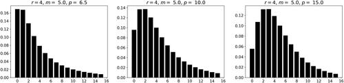
Figures 1 and 2 show the probability mass functions of ABM distributions with the same mean m = 5, the same power r = 4 of the variance function, but with increasing dispersion parameter p. When computing the features of these distributions, one observes decreasing zero probability, dispersion, skewness and kurtosis.

Figure 1. Probability mass functions of the ABM class for $r=4,m=5,$ and p = 1, 3, and 5, respectively.

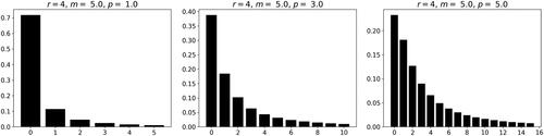
Figure 2. Probability mass functions of the ABM class for $r=4,m=5,$ and $p=6.5,10,$ and 15, respectively.

We obtain similar histograms in reversed order when mean m and dispersion p are fixed, and the variance function power r is increasing. Then, the distributions show increasing zero probability, dispersion, skewness and kurtosis.

3.3.2. LM class

Figures 3 and 4 show the probability mass functions of LMNS distributions with the same mean m = 2, the same power r = 4 of the variance function, but with increasing dispersion parameter p. Similar to the ABM distributions, we see decreasing zero probability, dispersion, skewness and kurtosis.

Figure 3. Probability mass functions of the LM class for $r=4,m=2,$ and $p=2.1,4,$ and 8, respectively.

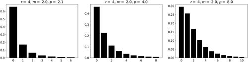
Figure 4. Probability mass functions of the LM class for $r=4,m=2,$ and p = 12, 16, and 20, respectively.

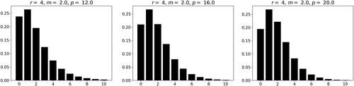
Again, when the variance function power r is increasing at a constant m and p, the distributions have increasing zero probability, dispersion, skewness and kurtosis.

4. Data applications

Well-known data sets that are used very often for validation and comparison reasons, concern automobile insurance claims because these show heavy overdispersion and zero inflation. Other sets can be found in diverse fields such as marketing, biometry, health and social sciences. In this section we investigate a number of these sets that were used in recent literature on the development of fitting models. We consider the following two-parameter models and their probability mass functions. These seven distributions are a mix of traditional ones, and some recently developed. We leave out models with one parameter, with three or more parameters, and regression models.

• PIG (Poisson-inverse Gaussian distribution) in Willmot (1987), $$p_n={\int }_0^{\infty }\frac{e^{-x} x^n}{n!} f(x;\beta ,\mu ) dx,n=0,1,\dots ,$$

where $f(x;\beta ,\mu )$ is the inverse Gaussion pdf with positive parameters β and μ.

• NLD (new logarithmic distribution) in Gomez-Deniz, Sarabia, and Calderin-Ojeda (2011), $$p_n=\frac{\hspace{0.17em}\text{log}\hspace{0.17em}(1-\alpha {\theta }^n)-\hspace{0.17em}\text{log}\hspace{0.17em}(1-\alpha {\theta }^{n+1})}{\hspace{0.17em}\text{log}\hspace{0.17em}(1-\alpha )}n=0,1,\dots ,$$

with parameters $\alpha <1$ ($\alpha \ne 0$), and $0<\theta <1.$

• NGDP (a new geometric discrete Pareto distribution) in Bhati and Bakouch (2019), $$p_n=\frac{q^n}{{(n+1)}^{\alpha }}-\frac{q^{n+1}}{{(n+2)}^{\alpha }},n=0,1,\dots ,$$

with parameters $0<q\le 1$ and $\alpha \ge 0.$

• EDLID (an exponentiated discrete Lindley distribution in from El-Morshedy, Eliwa, and Nagy (2020), $$p_n=\frac{1}{{(1-\hspace{0.17em}\text{log}\hspace{0.17em}a)}^b} (\Lambda (n+1;a,b)-\Lambda (n;a,b)),n=0,1,\dots ,$$

where $\Lambda (n;a,b)={(1-a^n+((1+n)a^n-1)\hspace{0.17em}\text{log}\hspace{0.17em}a)}^b,$ with parameters $0<a<1$ and b > 0.

• BTD (Bell-Touchard discrete distribution) in Castellares, Lemonte, and Moreno–Arenas (2020), $$p_n=\frac{1}{n!} e^{\theta (1-e^{\alpha })} {\alpha }^n{T}_n(\theta ),n=0,1,\dots ,$$

with positive parameters $\alpha ,\theta ,$ and where the $T_n(·)$ are Touchard polynomials; i.e, $$T_n(\theta )=e^{-\theta }\sum _{k=0}^{\infty }\frac{k^n {\theta }^k}{k!}$$

• ZIP (zero-inflated Poisson), in Lambert (1992), $$p_n=\{\begin{array}{cc}\pi +(1-\pi )e^{-\lambda },\hfill & \hspace{1em}n=0;\hfill \\ (1-\pi )e^{-\lambda }\frac{{\lambda }^n}{n!},\hfill & \hspace{1em}n=1,2,\dots \hfill \end{array}$$

where $0<\pi <1,$ and $\lambda >0.$

• PTD (Poisson-Tweedie distribution) in (Bonat et al. 2018; Kokonendji, Dossou-Gbété, and Demétrio 2004), $$p_n={\int }_0^{\infty }{e}^{-x}\frac{x^n}{n!} f_{\gamma }(x;p,t) dx,$$

where $f_{\gamma }(x;p,t)$ is a Tweedie density function with parameters p > 0, t < 0, $\gamma >2.$ The probabilities are computed by the recursion $$p_{n+1}=\frac{p{(\gamma -1)}^{\alpha -1}{(1-t)}^{\alpha -1}}{n+1}\sum _{j=0}^n\frac{\Gamma (j+1-\alpha )}{\Gamma (1-\alpha )j!} {(\frac{1}{1-t})}^j p_{n-j},$$

where $\alpha \in (0,1)$ satisfies $(\gamma -1)(1-\alpha )=1.$ We have included this distribution because it is associated to an exponential dispersion model with variance function $V(m)=m+p^{1-\gamma }{m}^{\gamma }$ which is an exponential function, similar to our classes. For a fixed exponent γ is it as a two-parameter distribution.

We applied maximum likelihood for estimating the parameters of all distributions. Concerning our distributions, we fix the power r in the range $\{1,\dots ,10\},$ we set the mean parameter $m=\overline{x},$ and then compute the dispersion parameter p by maximum likelihood estimation. We follow the same procedure for the Poisson-Tweedie distribution by fixing the power parameter γ.

4.1. Performance measures

Consider a data set of counts, $n_0,n_1,\dots ,n_K,$ meaning, n₀ observations of value 0, n₁ observations of value 1, etc. Let $N={\sum }_{k=0}^K{n}_k$ be the total number of observations. The empirical probability mass function is $$p_k^{(\text{emp})}=\frac{n_k}{N},k=0,\dots ,K.$$

We shall characterize such a data set by five features: zero mass, average, index of dispersion, skewness, and kurtosis. These are well-known, but for completeness we summarize them. Recall moments and central moments of order $r=1,2,\dots$ by $$m_r\doteq \frac{1}{N}\sum _{k=0}^K{k}^r{n}_k=\sum _{k=0}^K{k}^r{p}_k^{(\text{emp})},\hspace{1em}{m}_r^c\doteq \frac{1}{N}\sum _{k=0}^K{(k-m_1)}^r{n}_k=\sum _{k=0}^K{(k-m_1)}^r{p}_k^{(\text{emp})},$$ and that one usually denotes s² for the variance (central 2-nd moment $m_2^c$). Then, $$\begin{array}{c}\text{zeromass}{p}_0=p_0^{(\text{emp})}\\ \text{average}\overline{x}=m_1\\ \text{indexofdispersion}D=\frac{s^2}{\overline{x}}\\ \text{skewness}{b}_1=\frac{m_3^c}{s^3}\\ \text{kurtosis}{b}_2=\frac{m_4^c}{s^4}\end{array}$$

Furthermore, consider a (theoretical) probability model of a discrete random variable X on $\{0,1,\dots \}$ with probability mass function $$p_k^{(\text{mod})}\doteq \mathcal{P}(X=k), k=0,1,\dots .$$

The objective is to find a ‘good fitting’ model of the data. The performance of a model is expressed through the following measures.

• The logarithm of the likelihood: $$L=\hspace{0.17em}\text{log}\hspace{0.17em}\prod _{k=0}^K{n}_k{p}_k^{(\text{mod})}.$$

• ${\chi }^2$ value; taken into account sufficiently observations in the categories, which we have executed as follows. Since our data sets show zero-inflation with a rapidly decreasing tail, we take $s+1\le K$ categories, such that the categories $0,\dots ,s-1$ refer to the observed values $n_0,\dots ,n_{s-1},$ and category s groups all remaining values. Doing this as well for the fitting model, we arrive at $${\chi }^2=\sum _{k=0}^{s-1}\frac{{(n_k-N{p}_k^{(\text{mod})})}^2}{N{p}_k^{(\text{mod})}}+\frac{{(\sum _{k=s}^{\infty }{n}_k-N\sum _{k=s}^{\infty }{p}_k^{(\text{mod})})}^2}{N\sum _{k=s}^{\infty }{p}_k^{(\text{mod})}}.$$

• p-value of the ${\chi }^2$ quantile; taken into account the number of parameters that are estimated from the data. When there are s + 1 categories, and n_p parameters, the degrees of freedom (df) equals $s-n_p.$

• Root mean squared error (RMSE): $$\sqrt{\frac{1}{K+1}\sum _{k=0}^K(n_k-N{p}_k^{\text{mod}}{)}^2}.$$

• Kullback-Leibler divergence (KL): $$\sum _{k=0}^K{p}_k^{(\text{emp})} \hspace{0.17em}\text{log}\hspace{0.17em}\frac{p_k^{(\text{emp})}}{p_k^{(\text{mod})}}.$$

In the literature there are usages of a few other measures, such as mean square error (MSE), Akaike information criterion (AIC), or Bayesian information criterion (BIC). These are related to the measures mentioned earlier, and do not give more information.

4.2. Real data

We chose four data sets with various characteristics as summarized in Table 1. Data set 1 was considered in the literature for fitting by PIG, NLD, NGDP, and PTB, data set 2 by NGDP, data set 3 by EDLID, and data set 4 by NLD. Note that in this order of the sets, the zero mass probability, skewness and kurtosis are decreasing.

Table 1. Characteristics of data sets.

	p0	$\overline{x}$	D	b1	b2
Data set 1	0.9298	0.08650	1.417	5.316	41.01
Data set 2	0.7150	0.4831	2.092	3.163	16.34
Data set 3	0.5909	1.391	4.394	2.230	7.807
Data set 4	0.3322	1.708	2.148	1.707	6.904

4.2.1. Data set 1

Insurance claims in Zaire in 1974 (Gossiaux and Lemaire 1981) (Table 2).

Table 2. Data set 1.

Value	0	1	2	3	4	5
Frequency	3719	232	38	7	3	1

Table 3 summarizes the performances of the distributions that we mentioned earlier. We have computed our fitting models for power parameter r in the range of $r=1,\dots ,10.$ As selection criterion we used the chi-squared test on goodness-of-fit (Andrews 1988a, 1988b). This was the comparison measure for these data in Gossiaux and Lemaire (1981), and since then it has been considered for instance in Willmot (1987); Kokonendji and Khoudar (2004); Kokonendji, Dossou-Gbété, and Demétrio (2004). Thus, we choose the model that gave the the lowest ${\chi }^2$-value, equivalently, the one that gave the highest p-value. For the Poisson-Tweedie distribution we did a similar experiment concerning the power parameter γ, with step sizes 0.001.

Table 3. Performance of fitting data set 1.

Model	L	${\chi }^2$	df	p-value	RMSE	KL
PIG	–1183.52	0.543789	2	0.761935	1.760396	1.9866e-04
NLD	– 1183.97	2.312184	2	0.314714	2.235378	3.1047e-04
NGDP	–1183.44	0.383445	2	0.825536	1.303073	1.7734e-04
EDLID	– 1184.48	3.651826	2	0.161071	3.000701	4.3696e-04
BTD	–1186.20	9.251567	2	0.009796	4.056789	8.6835e-04
ZIP	–1187.78	14.771480	2	0.000620	5.313975	1.2621e-03
PTD($\gamma =2.684$)	–1183.39	0.437403	2	0.803561	1.053916	1.6459e-04
ABM(r = 10)	–1183.37	0.444316	2	0.800789	0.726210	1.5896e-04
LM(r = 4)	–1183.41	0.382719	2	0.825835	1.043140	1.6972e-04

When we consider the ${\chi }^2$ criterion, we find the best fit by the LM model (r = 4), however the ABM and model gives better (smaller) root mean squared error and Kullback-Leibler distance. The PIG and NGDP were proposed to model these data, and they are clearly performing as good as LM/ABM. Note that PTD is competetive in all criteria. The classic ZIP model shows bad performance, we will see this also in the other experiments.

4.2.2. Data set 2

The number of accidents experienced by machinists (Bliss and Fisher 1953) (Table 4).

Table 4. Data set 2.

Value	0	1	2	3	4	5	6	7	8
Frequency	296	74	26	8	4	4	1	0	1

Table 5 summarizes the performances. Also here, the ABM and LM models perform best, with PTD competing close. The NGDP was proposed to model these data, it gives also a good fit in all criteria. We found the best PTD for $\gamma =2.920$ close to γ = 3 in which case the PTD is in fact the PIG distribution. Indeed we see that the PTD performs slightly better than PIG.

Table 5. Performance of fitting data set 2.

Model	L	${\chi }^2$	df	p-value	RMSE	KL
PIG	–381.92	0.790146	3	0.851822	1.505635	6.0370e-03
NLD	– 382.13	2.292750	3	0.513911	1.732206	6.5419e-03
NGDP	–381.82	1.302363	3	0.728572	1.251828	5.7786e-03
EDLID	– 382.97	4.198396	3	0.240822	2.585325	8.5663e-03
BTD	–386.46	11.293501	3	0.010240	3.786089	1.4734e-02
ZIP	–391.63	27.329394	3	0.000005	5.714534	2.9491e-02
PTD($\gamma =2.920$)	–381.88	0.784300	3	0.853218	1.394523	5.9263e-03
ABM(r = 10)	–381.80	0.891831	3	0.827399	1.036148	5.7331e-03
LM(r = 3)	–381.95	0.753439	3	0.860568	1.297283	6.0981e-03

4.2.3. Data set 3

The counts of cysts of kidneys using steroids (Chan et al. 2010) (Table 6).

Table 6. Data set 3.

Value	0	1	2	3	4	5	6	7	8	9	10	11
Frequency	65	14	10	6	4	2	2	2	1	1	1	2

Table 7 summarizes the performances. The EDLID was proposed to model these data, it gives indeed the best fit. The ABM-r = 1 and PTD-γ =  =nd PTD-indeed the best fit. The ABM- ABM-proposed to model these data, it gives indeed the best fit. The ABM-lham, A. S. Woolf, and D. A. L

Table 7. Performance of fitting data set 3.

Model	L	${\chi }^2$	df	p-value	RMSE	KL
PIG	–170.87	4.754522	3	0.190680	2.762842	6.3329e-02
NLD	– 167.52	0.705282	3	0.871961	1.038579	3.2884e-02
NGDP	–168.87	2.530106	3	0.469875	2.243219	4.5103e-02
EDLID	– 166.95	0.151495	3	0.985011	0.665346	2.7689e-02
BTD	–170.91	4.485663	3	0.213573	2.108909	6.3666e-02
ZIP	–182.24	15.768584	3	0.001265	3.238417	1.6673e-01
PTD(γ = 2)	–167.54	0.632639	3	0.888921	1.034530	3.3090e-02
ABM(r = 1)	–167.54	0.632639	3	0.888921	1.034530	3.3090e-02
LM(r = 10)	–171.01	4.762802	3	0.190013	2.717090	6.4574e-02

4.2.4. Data set 4

Number of claims of automobile liability policies (Klugman, Panjer, and Willmot 1998) (Table 8).

Table 8. Data set 4.

Value	0	1	2	3	4	5	6	7	8	9	10	11
Frequency	99	65	57	35	20	10	4	0	3	4	0	1

Table 9 summarizes the performances. The NLD was proposed to model these data, and it gives indeed a good fit, but also distribution EDLID. Remarkebly, the BTD performs excellent. The data set shows low zero-inflation and low higher moments, resulting that our models are not as good.

Table 9. Performance of fitting data set 4.

Model	L	${\chi }^2$	df	p-value	RMSE	KL
PIG	–530.10	6.659803	4	0.154996	6.194263	3.6346e-02
NLD	– 528.40	2.408122	4	0.661160	3.527420	3.0641e-02
NGDP	–531.46	10.267733	4	0.036151	5.863542	4.0934e-02
EDLID	– 528.56	3.029695	4	0.552868	3.734667	3.1208e-02
BTD	–529.93	1.025681	4	0.905877	2.292173	2.9729e-02
ZIP	–542.67	12.091699	4	0.016682	5.288587	7.8550e-02
PTD(γ = 2)	–528.77	3.680797	4	0.450925	4.247745	3.1895e-02
ABM(r = 1)	–528.77	3.680797	4	0.450925	4.247745	3.1895e-02
LM(r = 10)	–529.65	5.682523	4	0.224145	5.674060	3.4849e-02

4.3. Simulated data

We saw in the results of our models in comparison with recently proposed others, that the larger zero-mass probability, skewness, and kurtosis data have, the better our models perform. When these data characteristics are rather large, our models outperform even models that were proposed for fitting these data sets. When the data characteristics are rather small, our models may be competitive, but they seem not to be the best for fitting purposes compared to the other models that we considered.

For testing this hypothesis we have executed an extensive numerical study on a total of 20 data sets found in literature, see our report Bar-Lev and Ridder (2020) which is available on the arXiv. When we order these sets by decreasing skewness and kurtosis, and when we consider the ${\chi }^2$ and p-value performances, the first 13 data were fitted best by ABM or LMNS with one exception. The last 7 data were fitted best by (one of) the other four models.

For further testing our claim that our models are suitable for fitting purposes when data show high zero-inflation, skewness and kurtosis, we ran a simulation experiment. First we constructed a probability distribution on a finite support having the required properties of zero-mass and the first four moments. The probability distribution was obtained by applying the maximum entropy method with these constraints (Jaynes 1957). From the distribution we generated N = 10000 simulated data, and then apply our fitting models to these data. We present here three data sets that were simulated in this manner. All data have values $0,\dots ,K=8$ (Table 10).

Table 10. Three sets of simulated data.

Value	0	1	2	3	4	5	6	7	8
Data set 5	8203	1417	290	62	19	5	0	3	1
Data set 6	7933	1420	406	132	63	23	16	4	3
Data set 7	4624	2387	1390	752	412	211	103	74	47

The first two sets were obtained from distributions with relative large zero-mass, skewness and kurtosis, see the characteristics in Table 11, though the second set is slightly more flat. The third set is much more flat with relative small zero-mass, skewness and kurtosis.

Table 11. Characteristics of simulated data sets.

	p0	$\overline{x}$	D	b1	b2
Data set 5	0.8203	0.2313	1.401	3.481	22.25
Data set 6	0.7933	0.3143	1.843	3.569	20.40
Data set 7	0.4624	1.164	2.009	1.702	6.126

Finally, the performances of our ABM and LM models against the seven models that we consider in our study for comparisons, are summarized in Tables 12–14. The results confirm our suggestion that our models are well-suited for fitting zero-inflated overdispersed data with relative large skewness and kurtosis. Moreover, ABM is more suited than LM when the tail is flatter.

Table 12. Performance of fitting data set 5.

Model	L	${\chi }^2$	df	p-value	RMSE	KL
PIG	–5931.76	1.035150	3	0.792748	4.648578	5.4929e-04
NLD	– 5936.02	5.965423	3	0.113305	9.971059	9.7550e-04
NGDP	–5934.05	3.220770	3	0.358823	9.859480	7.7833e-04
EDLID	– 5939.82	12.760586	3	0.005184	14.395989	1.3553e-03
BTD	–5947.82	29.654061	3	0.000002	19.082800	2.0303e-03
ZIP	–5966.77	95.916546	3	0.000000	29.550924	4.0501e-03
PTD($\gamma =2.812$)	–5931.90	0.909689	3	0.823089	3.483411	5.6369e-04
ABM(r = 10)	–5932.31	1.198908	3	0.753266	4.490144	6.0485e-04
LM(r = 2)	–5931.53	0.723555	3	0.867650	3.297800	5.2608e-04

Table 13. Performance of fitting data set 6.

Model	L	${\chi }^2$	df	p-value	RMSE	KL
PIG	–7106.28	6.023648	4	0.197389	19.786444	7.9821e-04
NLD	– 7107.42	15.922941	4	0.003124	20.825278	9.1194e-04
NGDP	–7102.73	2.192939	4	0.700322	4.990708	4.4282e-04
EDLID	– 7117.12	40.313621	4	0.000000	34.229900	1.8821e-03
BTD	–7149.64	147.108365	4	0.000000	52.296407	5.1338e-03
ZIP	–7207.74	510.837458	4	0.000000	77.450065	1.0944e-02
PTD($\gamma =2.513$)	–7102.73	1.732954	4	0.784723	5.734922	4.4270e-04
ABM(r = 6)	–7103.02	1.669665	4	0.796220	5.126902	4.7231e-04
LM(r = 10)	–7104.07	2.311162	4	0.678738	9.632771	5.7683e-04

Table 14. Performance of fitting data set 7.

Model	L	${\chi }^2$	df	p-value	RMSE	KL
PIG	–14995.75	99.083792	5	0.000000	149.291054	1.0650e-02
NLD	– 14934.82	11.271396	5	0.046257	52.119898	4.5567e-03
NGDP	–14936.26	10.581946	5	0.060329	40.518667	4.7004e-03
EDLID	– 14924.71	2.381891	5	0.794168	13.910594	3.5448e-03
BTD	–14946.95	74.021500	5	0.000000	78.646023	5.7693e-03
ZIP	–15205.17	968.884983	5	0.000000	221.474368	3.1591e-02
PTD(γ = 2)	–14935.23	11.539940	5	0.041665	51.234138	4.5976e-03
ABM(r = 1)	–14935.23	11.539940	5	0.041665	51.234138	4.5976e-03
LM(r = 10)	–14980.33	71.569157	5	0.000000	126.322372	9.1075e-03

Table 12 summarizes the performances for fitting data set 5. For this data set with high skewness and kurtosis, and large zero-inflation, we found excellent fitting by the LM class. Note also the competitive perfromance of PTD with power parameter γ close to 3, and therefore the PIG is not too bad. Most other distributions are not suited to model such data.

Table 13 summarizes the performances for fitting data set 6. Here we see that an ABM distribution has the best fit when considering the p-value criterion, but for the other criteria, either the NGDP or the PTD perform best. Most other distributions perform basdly.

Table 14 summarizes the performances for fitting data set 7. Remarkebly all but one model (EDLID) has difficulty with finding a good fit. The data set is rather flat with relative low zero-inflation and low higher moments.

5. Conclusion

In this paper we investigated two classes of exponential dispersion models for fitting data sets showing zero-dispersion and overdispersion. These models act as alternatives not only to classic distributions such as Poisson, generalized Poisson, negative binomial, discrete Lindley, and Poisson-inverse Gaussian, but also to recently proposed models, such as discrete Gamma, discrete Rayleigh, new logarithmic, geometric discrete Pareto, and exponentiated discrete Lindley, to name a few. Our two classes are given by specifying their variance functions in the mean parameterization of their exponential forms. The variance functions are particular polynomials of the mean. This is a convenient and flexible way of specifying families of probability distributions, namely by a functional form of the first two moments. Moreover, we were able to to develop a numerical procedure to compute the actual associated probability distributions. Further investigation of these distributions showed that they show a monotonic behavior for zero-inflation, skewness, and kurtosis, by varying the dispersion parameter, or by varying the degree of the variance polynomials. Finally, the main purpose was to determine how good fits our models are to discrete count data such as insurance claims. We executed an extensive numerical study on twenty real data sets, four of which are reported in this paper, and on three sets of simulated data, where we compared our models with four recently developed in the literature. The conclusion is that our models are very well suited to fit zero-inflated overdispersed data with large skewness and kurtosis.

Acknowledgements

The authors are grateful to the reviewers for their comments and suggestions for improvements.

Additional information

Funding

Shaul Bar-Lev was partially supported in this research by the Netherlands Organization for Scientific Research (NWO), project number 040.11.711.

References

- Alamatsaz, M. H., S. Deey, T. Dey, and S. Shams Harandi. 2016. Discrete generalized Rayleigh distribution. Pakistan Journal of Statistics 32 (1):1–20.
- Andrews, D. 1988a. Chi-square diagnostic tests for Econometric models: Introduction and application. Journal of Econometrics 37 (1):135–56. doi:10.1016/0304-4076(88)90079-6.
- Andrews, D. 1988b. Chi-square diagnostic tests for Econometric models: Theory. Econometrica 56 (6):1419–53. doi:10.2307/1913105.
- Armeli, S., C. Mohr, M. Todd, N. Maltby, H. Tennen, M. A. Carney, and G. Affleck. 2005. Daily evaluation of anticipated outcomes from alcohol use Aamong college students. Journal of Social and Clinical Psychology 24 (6):767–92. doi:10.1521/jscp.2005.24.6.767.
- Awad, Y., S. K. Bar-Lev, and, and U. Makov. 2016. A new class counting distributions embedded in the Lee-Carter model for mortality projections: A Bayesian approach. Technical report No. 146, Actuarial Research Center, University of Haifa, Israel.
- Bar-Lev, S. K., and C. C. Kokonendji. 2017. On the mean value parameterization of natural exponential families - a revisited review. Mathematical Methods of Statistics 26 (3):159–75. doi:10.3103/S1066530717030012.
- Bar-Lev, S. K., and A. Ridder. 2019. Monte Carlo methods for insurance risk computation. International Journal of Statistics and Probability 8 (3):54–74. doi:10.5539/ijsp.v8n3p54.
- Bar-Lev, S. K., and A. Ridder. 2020. Supplementary data analyses of exponential dispersion models for overdispersed zero-inflated count data. Available as arXiv:2003.13854.
- Bar-Lev, S. K., and A. Ridder. 2021. New exponential dispersion models for count data - the ABM and LM classes. ESAIM: Probability and Statistics 25:31–52. doi:10.1051/ps/2021001.
- Barndorff-Nielsen, O. 1978. Information and exponential families in statistical theory. Chichester: Wiley.
- Bhati, D., and H. S. Bakouch. 2019. A new infinitely divisible discrete distribution with applications to count data modelling. Communications in Statistics - Theory and Methods 48 (6):1401–16. doi:10.1080/03610926.2018.1433847.
- Bliss, C. I., and R. A. Fisher. 1953. Fitting the negative binomial distribution to biological data. Biometrics 9 (2):176–200. doi:10.2307/3001850.
- Bonat, W. H., B. Jørgensen, C. C. Kokonendji, J. Hinde, and C. G. B. Demétrio. 2018. Extended poisson–tweedie: Properties and regression models for count data. Statistical Modelling 18 (1):24–49. doi:10.1177/1471082X17715718.
- Castellares, F., A. J. Lemonte, and G. Moreno–Arenas. 2020. On the two-parameter Bell–Touchard discrete distribution. Communications in Statistics - Theory and Methods 49 (19):4834–52. doi:10.1080/03610926.2019.1609515.
- Chakraborty, S., and D. Chakravarty. 2012. Discrete Gamma distributions: Properties and parameter estimations. Communications in Statistics - Theory and Methods 41 (18):3301–24. doi:10.1080/03610926.2011.563014.
- Chan, S.-K., P. R. Riley, K. L. Price, F. McElduff, P. J. Winyard, S. J. M. Welham, A. S. Woolf, and D. A. Long. 2010. Corticosteroid-induced kidney dysmorphogenesis is associated with deregulated expression of known cystogenic molecules, as well as indian hedgehog. American Journal of Physiology-Renal Physiology 298 (2):F346–356. doi:10.1152/ajprenal.00574.2009.
- Coly, S., A.-F. Yao, D. Abrial, and M. Charras-Garrido. 2016. Distributions to model overdispersed count data. Journal de la Société Française de Statistique 157 (2):39–63.
- Consul, P. C. 1989. Generalized poisson distributions: Properties and applications. New York: Marcel Dekker.
- El-Morshedy, M., M. S. Eliwa, and H. Nagy. 2020. A new two-parameter exponentiated discrete Lindley distribution: Properties, estimation and applications. Journal of Applied Statistics 47 (2):354–75. doi:10.1080/02664763.2019.1638893.
- Fahrmeir, L., and L. Osuna Echavarría. 2006. Structured additive regression for overdispersed and zero-inflated count data. Applied Stochastic Models in Business and Industry 22 (4):351–69. doi:10.1002/asmb.631.
- Gomez-Deniz, E., and E. Calderin-Ojeda. 2011. The discrete Lindley distribution: Properties and applications. Journal of Statistical Computation and Simulation 81:1405–16.
- Gomez-Deniz, E., J. M. Sarabia, and E. Calderin-Ojeda. 2011. A new discrete distribution with actuarial applications. Insurance: Mathematics and Economics 48 (3):406–12. doi:10.1016/j.insmatheco.2011.01.007.
- Gossiaux, A., and J. Lemaire. 1981. Methodes d’ajustement de distributions de sinistres. Bulletin of the Association of Swiss Actuaries 81:87–95.
- Hinde, J., and C. G. B. Demétrio. 1998. Overdispersion: Models and estimation. Computational Statistics & Data Analysis 27 (2):151–70. doi:10.1016/S0167-9473(98)00007-3.
- Jain, G. C., and P. C. Consul. 1971. A generalized negative binomial distribution. SIAM Journal on Applied Mathematics 21 (4):501–13. doi:10.1137/0121056.
- Jaynes, E. T. 1957. Information theory and statistical mechanics. Physical Review 106 (4):620–30. doi:10.1103/PhysRev.106.620.
- Jørgensen, B. 1997. The theory of exponential dispersion models, Monograph on statistics and probability. Vol. 76. London: Chapman and Hall.
- Jørgensen, B., and C. C. Kokonendji. 2016. Discrete dispersion models and their Tweedie asymptotics. AStA Advances in Statistical Analysis 100 (1):43–78. doi:10.1007/s10182-015-0250-z.
- Klugman, S., H. Panjer, and G. Willmot. 1998. Loss models. From data to decisions. 3rd ed. New York: John Wiley and Sons.
- Kokonendji, C. C., S. Dossou-Gbété, and C. G. B. Demétrio. 2004. Some discrete exponential dispersion models: Poisson-Tweedie and Hinde-Demétrio classes. Statistics and Operations Research Transactions 28 (2):201–14.
- Kokonendji, C. C., and M. Khoudar. 2004. On strict arcsine distribution. Communications in Statistics - Theory and Methods 33 (5):993–1006. doi:10.1081/STA-120029820.
- Lambert, D. 1992. Zero-inflated Poisson regression, with an application to defects in manufacturing. Technometrics 34 (1):1–14. doi:10.2307/1269547.
- Letac, G., and M. Mora. 1990. Natural real exponential families with cubic variance functions. The Annals of Statistics 18 (1):1–37. doi:10.1214/aos/1176347491.
- Lord, D., S. P. Washington, and J. N. Ivan. 2005. Poisson, poisson-gamma and zero-inflated regression models of motor vehicle crashes: Balancing statistical fit and theory. Accident Analysis & Prevention 37 (1):35–46. doi:10.1016/j.aap.2004.02.004.
- Ridout, M., J. Hinde, and C. G. B. Demétrio. 2001. A score test for testing a zero-inflated Poisson regression model against zero-inflated negative binomial alternatives. Biometrics 57 (1):219–23. doi:10.1111/j.0006-341X.2001.00219.x.
- Siddiqui, O., J. Mott, T. Anderson, and B. Flay. 1999. The application of Poisson random-effects regression models to the analyses of adolescents’ current level of smoking. Preventive Medicine 29 (2):92–101. doi:10.1006/pmed.1999.0517.
- Walters, G. D. 2007. Predicting institutional adjustment with the lifestyle criminality screening form and the antisocial features and aggression scales of the PAI. Journal of Personality Assessment 88 (1):99–105. doi:10.1080/00223890709336840.
- Willmot, G. 1987. The Poisson-inverse Gaussian distribution as an alternative to the negative binomial. Scandinavian Actuarial Journal 1987 (3-4):113–27. doi:10.1080/03461238.1987.10413823.
- Yip, K. C. H., and K. K. W. Yau. 2005. On modelling claim frequency data in general insurance with extra zeros. Insurance: Mathematics and Economics 36 (2):153–63. doi:10.1016/j.insmatheco.2004.11.002.
- Zafakali, N. S., and W. M. A. W. Ahmad. 2013. Modelling and handling overdispersion health science data with zero-inflated Poisson model. Journal of Modern Applied Statistical Methods 12 (1):255–60. doi:10.22237/jmasm/1367382420.
- Zhao, X., and X. Zhou. 2012. Copula models for insurance claim numbers with excess zeros and time-dependence. Insurance: Mathematics and Economics 50 (1):191–9. doi:10.1016/j.insmatheco.2011.11.004.