Generalized two-parameter estimators in the multinomial logit regression model: methods, simulation and application

Abstract

In this article, we propose generalized two-parameter (GTP) estimators and an algorithm for the estimation of shrinkage parameters to combat multicollinearity in the multinomial logit regression model. In addition, the mean squared error properties of the estimators are derived. A simulation study is conducted to investigate the performance of proposed estimators for different sample sizes, degrees of multicollinearity, and the number of explanatory variables. Swedish football league dataset is analyzed to show the benefits of the GTP estimators over the traditional maximum likelihood estimator (MLE). The empirical results of this article revealed that GTP estimators have a smaller mean squared error than the MLE and can be recommended for practitioners.

Keywords:

• Generalized two-parameter estimators
• MSE
• Multicollinearity
• Multinomial logistic regression
• Simulation
• Swedish football league

1. Introduction

The multinomial logit regression (MNLR) model introduced by Luce (1959) and is often used when the dependent variable comprises more than two categories. Mostly, the MNLR is used to model nominal output variables in which the log odds of the outputs are modeled as a linear combination of explanatory variables. Nowadays, the MNLR is a very common choice among applied researchers for analyzing the categorical response variable having at least three categories. For example, blood types of humans and animals give different diagnostic tests, determination of socioeconomic factors that affect major choices made by consumers, getting unrestricted credit, restricted credit, or no credit by different corporations due to their financial and official characteristics and among others. It is a general practice to use an ordinary maximum likelihood estimator (MLE) to estimate the parameters vector of the MNLR. Multicollinearity is a situation in MNLR where two or more explanatory variables are highly correlated with each other. The problem of multicollinearity can have numerous adverse effects on regression coefficients. The main drawback of multicollinearity is that the variance of the MLE becomes inflated (Månsson et al., 2018). In addition, on average estimates are too large and can have wrong signs of the estimated parameters. Consequently, the probability of type-II error of estimated parameter will be increased, which result in decreased statistical power; the Wald statistic gives insignificant results in the presence of multicollinearity (Qasim, Kibria, et al. 2020a).

Different biased estimation methods have been proposed to solve the problem of multicollinearity for a different type of regression models. Some of the biased estimation methods for popular regression models are: Hoerl and Kennard (1970) proposed a ridge regression (RR) estimator to deal the problem of multicollinearity for the linear regression model (LRM). Schaefer, Roi, and Wolfe (1984), Schaefer (1986) introduced ridge regression and Stein estimators for the logistic regression model. Kejian (1993, 2003) proposed a Liu and Liu-type estimators for the LRM. Månsson and Shukur (2011a) and Månsson, Kibria, and Shukur (2012) developed ridge regression and Liu estimators for the logit regression model, respectively. Månsson and Shukur (2011b), Qasim, Kibria, et al. (2020a), Qasim, Månsson, et al. (2020b), Lukman et al. (2020) and Noori Asl et al. (2020) suggested Poisson RR, Poisson Liu regression, biased adjusted Poisson RR, modified Poisson ridge-type, and penalized and ridge-type shrinkage estimators in the Poisson regression model, respectively. Månsson (2012, 2013) introduced ridge negative binomial ridge and Liu regression estimators, respectively. Kurtoğlu and Özkale (2016), Qasim, Amin, and Amanullah (2018), Mandal et al. (2019), Amin, Qasim, Yasin, et al. (2020b), Amin, Qasim, Amanullah, et al. (2020a) and Lukman et al. (2020) developed Liu estimation, Liu shrinkage parameters, Stein-type shrinkage estimators, bias and almost unbiased RR and modified ridge-type estimators for the gamma regression, respectively. Karlsson, Månsson, and Kibria (2020) and Qasim, Månsson, and Golam Kibria (2021) proposed beta Liu and ridge regression estimators, respectively.

Özkale and Kaciranlar (2007) proposed a two-parameter biased estimator by grafting contraction estimator into modified RR estimator in the LRM. They stated that as the value of k (ridge parameter) becomes increases then the RR has an unnecessary amount of bias. Yang and Chang (2010) suggested another efficient two-parameter estimator. Toker, Üstündağ Şiray, and Qasim (2019) proposed a first-order two-parameter estimator in the generalized linear models (GLM). Regarding the considerable literature on a two-parameter estimator for a different form of the GLM, we refer to Huang and Yang (2014), Asar and Genç (2018), Abonazel and Farghali (2019), Rady, Abonazel, and Taha (2019), Amin, Qasim, and Amanullah (2019), Farghali (2019), Akram, Amin, and Qasim (2020), Naveed et al. (2020) and among others. El-Dash, El-Hefnawy, and Farghali (2011) proposed Stein-type ridge regression and generalized ridge regression estimators for the MNLR and Månsson et al. (2018) suggested ridge estimators for the MNLR. By extending the work of Månsson, Kibria, and Shukur (2012), Farghali (2014) proposed a multinomial Liu estimator. Asl et al. (2021) proposed the Stein-type shrinkage ridge estimator when the regression coefficients are restricted to a linear subspace in the GLM and derive the asymptotic biases and risks of the proposed estimators.

The main purpose of this article is to develop two different generalized two-parameter (GTP) estimators for the MNLR by following the work of Abonazel and Farghali (2019) and Yang and Chang (2010). In addition, we suggest a new algorithm for the selection of optimal shrinkage parameters $\left(k_j \mathit{and} d_j\right)$ for GTP estimators. The proposed GTP estimators are general estimators which include the MLE, RR, generalized RR, Liu estimator, and generalized Liu-type estimator. The mean square error (MSE) properties of the estimators are examined and show the superiority of the proposed estimators under certain conditions. Besides, the Monte Carlo simulation and Swedish football league dataset are analyzed to demonstrate the benefit of the proposed estimators over the existing classical MLE.

The rest of the article is arranged as follows: The MNLR model, GTP estimators and MSE properties are well defined in Sec. 2. Estimation methods for selection of generalized optimal shrinkage parameters are explained in Sec. 3. Simulation experiment and their results are discussed in Sec. 4. The advantage of our recommended estimators is demonstrated by analyzing empirical application in Sec. 5 and finally, some concluding remarks are given in Sec 6.

2. Model and proposed GTP estimators

This section illustrates the methodology of the MNLR and MLE. In addition, we propose two new GTP estimators by considering the work of Abonazel and Farghali (2019), and Huang and Yang (2014) in the MNLR model.

2.1. Multinomial logit regression

The multinomial logistic regression model assumes that the response variable $y$ has a multinomial distribution. Consider a trial that results in exactly one of some fixed finite number of $C$ possible outcomes, with probabilities ${\pi }_1,$${\pi }_2,$…$, {\pi }_C,$$0\le {\pi }_h\le 1,$ $h=1,2,\dots ,C$ and ${\sum }_{h=1}^C{\pi }_h=1$. The random variable $y_i=(y_{i1}, y_{i2},.{.y}_{ih}\dots ,y_{iC})$ for n independent trials represents the multinomial trial for observation $i \left(i=1,2,\dots ,n\right)$ and $y_{ih}$ takes the following values: $$y_{ih}=\{\begin{array}{cc}1& \text{the }{i\mathrm{th}}^{}\text{ observation }\in \text{ the }{h\mathrm{th}}^{}\mathrm{ }\mathrm{level}\\ 0& \mathrm{otherwise}\end{array},\mathrm{ }i=1,2,\dots ,n,\mathrm{ }h=1,\dots ,C$$

Thus, ${\sum }_{h=1}^C{y}_{ih}=1.$ The probability density function of multinomial distribution is defined as (1) $$f(y_{i1},\dots ,y_{iC})=\frac{n!}{y_{i1}!\dots ,y_{iC}!}{\pi }_1(x_i{)}^{y_{i1}}.{\pi }_h(x_i{)}^{y_{ih}}.{\pi }_C(x_i{)}^{y_{iC}},$$(1) where${\sum }_{h=1}^C{y}_{ih}=1 \therefore { y}_{iC}=1-{\sum }_{h=1}^{C-1}{y}_{ih}.$ Using the value of $y_{iC}$ in (1) the density function can be written as $$f(y_{i1},\dots ,y_{iC})=\mathrm{ }\frac{n!}{y_{i1}!.,(1-{\sum }_{h=1}^{C-1}{y}_{ih})!}{\pi }_1(x_i{)}^{y_{i1}}..{\pi }_h(x_i{)}^{y_{ih}}..{\pi }_C(x_i{)}^{\left(1-\sum _{h=1}^{C-1}{y}_{ih}\right)}.$$

To develop the MNLR, assume that the explanatory variables $x_1,x_2,\dots ,x_p$ are measured for observations $y_{i1},\dots ,y_{iC}$ which follow a multinomial distribution with probability parameters${\pi }_1,$${\pi }_2,$…$,{\pi }_C .$ Then the conditional probabilities of each response variables’ level given the explanatory variables vector are $${\pi }_h\left(x_i\right)=\mathrm{Pr}(Y=h|x_1,x_2,\dots ,x_p)=\frac{e^{{\beta }_{h0}+{\sum }_{j=1}^p{\beta }_{hj}{x}_{ij}}}{1+{\sum }_{h=1}^{C-1}{e}^{{\beta }_{h0}+{\sum }_{j=1}^p{\beta }_{hj}{x}_{ij}}},\mathrm{ }h=1,2,\dots ,C-1$$ $${\pi }_C\left({\mathrm{x}}_i\right)=\frac{1}{1+{\sum }_{h=1}^{C-1}{e}^{{\beta }_{h0}+{\sum }_{j=1}^p{\beta }_{hj}{x}_{ij}}}.$$

Thus, the MNLR is (2) $$\mathit{ln}\left[\frac{{\pi }_h\left(x_i\right)}{{\pi }_C\left(x_i\right)}\right]={\beta }_{h0}+{\sum }_{j=1}^p{\beta }_{hj}\mathrm{ }{x}_{ij},\mathrm{ }h=1,2,\dots ,C-1,\mathrm{ }i=1,2,\dots ,n.$$(2) where $n$ is the sample size, $p$ is the number of explanatory variables, $C$ is the number of levels of the response variable (in model (2) level $C$ is the reference level), ${\beta }_{h0},{\beta }_{hj}\text{ are the regression}$ parameters at the $h^{th}$ level of the response variable.

The most common method for estimating the model parameters is to apply the MLE, which maximizes the log-likelihood function

$$L=\prod _{i=1}^n\frac{n!}{y_{i1}!\times y_{i2}!\times ...\times (1-{\sum }_{\mathrm{h}=1}^{C-1}{y}_{ih})!}{\left[\frac{{\widehat{\pi }}_1\left(x\right)}{{\widehat{\pi }}_C\left(x\right)}\right]}^{y_{i1}}\times {\left[\frac{{\widehat{\pi }}_2\left(x\right)}{{\pi }_C\left(x\right)}\right]}^{y_{i2}}\times \cdots \times {\left[\frac{{\widehat{\pi }}_h\left(x\right)}{{\widehat{\pi }}_C\left(x\right)}\right]}^{y_{ih}}\dots \times {\widehat{\pi }}_C\left(x\right).$$$$\ln L=\sum _{i=1}^n\left[\ln \left(\frac{n!}{y_{i1}!\times ...\times (1-{\sum }_{\mathrm{h}=1}^{C-1}{y}_{ih})!}\right)+y_{i1}\ln \left[\frac{{\widehat{\pi }}_1\left(x\right)}{{\widehat{\pi }}_C\left(x\right)}\right]+y_{i2}\ln \left[\frac{{\widehat{\pi }}_2\left(x\right)}{{\widehat{\pi }}_C\left(x\right)}\right]+...+\ln {\widehat{\pi }}_C\left(x\right)\right].$$

Let $A=\ln \left(\frac{n!}{y_{i1}!\times y_{i2}!\times ...\times (1-{\sum }_{\mathrm{h}=1}^{C-1}{y}_{ih})!}\right)$.

Then $$\ln L={\sum }_{i=1}^n{\sum }_{\mathrm{h}=1}^{C-1}\left[A+y_{i1}\mathit{ln}\left[\frac{{\widehat{\pi }}_1\left(x\right)}{{\widehat{\pi }}_C\left(x\right)}\right]+y_{i2}\ln \left[\frac{{\widehat{\pi }}_2\left(x\right)}{{\widehat{\pi }}_C\left(x\right)}\right]+...+\ln {\widehat{\pi }}_C\left(x\right)\right]$$ $$\ln L=\sum _{i=1}^n\sum _{h=1}^{C-1}\left(A+y_{ih}\mathrm{ }\ln \left(\frac{{\pi }_h\left(x_i\right)}{{\pi }_C\left(x_i\right)}\right)+\ln \left({\pi }_C\left(x_i\right)\right)\right)$$ (3) $$\ln L={\sum }_{i=1}^n{\sum }_{h=1}^{C-1}\left[{A+y}_{ih}\left({\beta }_{h0}+{\sum }_{j=1}^p{\beta }_{hj}\mathrm{ }{x}_{ij}\right)+\ln \left(\frac{1}{1+{\sum }_{h=1}^{C-1}{e}^{{\beta }_{h0}+{\sum }_{j=1}^p{\beta }_{hj}\mathrm{ }{x}_{ij}}}\right)\right]$$(3)

The MLE can be found by setting the first derivative of (3) to zero. Thus, ${\widehat{\beta }}_{\mathit{MLE}}$ is obtained by solving the following nonlinear system of equations: (4) $$\sum _{i=1}^n{y}_{ih}=\sum _{i=1}^n\left(\frac{e^{{\beta }_{h0}+{\sum }_{j=1}^p{\beta }_{hj}\mathrm{ }{x}_{ij}}}{1+{\sum }_{h=1}^{C-1}{e}^{{\beta }_{h0}+{\sum }_{j=1}^p{\beta }_{hj}\mathrm{ }{x}_{ij}}}\right),\mathrm{ }h=1,\dots ,C-1.$$(4) (5) $$\sum _{i=1}^n{y}_{ih}{x}_{ij}=\sum _{i=1}^n\left(\frac{e^{{\beta }_{h0}+{\sum }_{j=1}^p{\beta }_{hj}\mathrm{ }{x}_{ij}}}{1+{\sum }_{h=1}^{C-1}{e}^{{\beta }_{h0}+{\sum }_{j=1}^p{\beta }_{hj}\mathrm{ }{x}_{ij}}}\right)\mathrm{ }{x}_{ij},\mathrm{ }h=1,\dots ,C-1.\mathrm{ }$$(5)

The solution to Equations (4)(4) $$\sum _{i=1}^n{y}_{ih}=\sum _{i=1}^n\left(\frac{e^{{\beta }_{h0}+{\sum }_{j=1}^p{\beta }_{hj}\mathrm{ }{x}_{ij}}}{1+{\sum }_{h=1}^{C-1}{e}^{{\beta }_{h0}+{\sum }_{j=1}^p{\beta }_{hj}\mathrm{ }{x}_{ij}}}\right),\mathrm{ }h=1,\dots ,C-1.$$(4) and (5)(5) $$\sum _{i=1}^n{y}_{ih}{x}_{ij}=\sum _{i=1}^n\left(\frac{e^{{\beta }_{h0}+{\sum }_{j=1}^p{\beta }_{hj}\mathrm{ }{x}_{ij}}}{1+{\sum }_{h=1}^{C-1}{e}^{{\beta }_{h0}+{\sum }_{j=1}^p{\beta }_{hj}\mathrm{ }{x}_{ij}}}\right)\mathrm{ }{x}_{ij},\mathrm{ }h=1,\dots ,C-1.\mathrm{ }$$(5) is found by applying numerical methods such as Newton- Raphson or scoring method see Agresti (2013) and Hosmer, Lemeshow, and Sturdivant (2013) and $\mathit{the}$ asymptotic variance-covariance matrix of ${\widehat{\beta }}_{\mathit{MLE}}$ is calculated as follows: $$\mathit{Cov}\left({\widehat{\beta }}_{\mathit{MLE}}\right)={\left(X^{\mathrm{\prime }}\widehat{W}X\right)}^{-1}=\left(\begin{array}{ccc}X\mathrm{\prime }{\widehat{w}}_{11}X& \begin{array}{cc}-X\mathrm{\prime }{\widehat{w}}_{12}X& \mathrm{ }\dots \end{array}& -X\mathrm{\prime }{\widehat{w}}_{1(C-1)}X\\ ⋮& \mathrm{ }\ddots & ⋮\\ -X\mathrm{\prime }{\widehat{w}}_{(C-1)1}X& \begin{array}{cc}-X\mathrm{\prime }{\widehat{w}}_{(C-1)2}X& \dots \end{array}& X\mathrm{\prime }{\widehat{w}}_{(C-1)(C-1)}X\end{array}\right)$$ where $X$ is a $n\times p^{*}$ matrix of the explanatory variables which the first column contains one and $p^{*}=p+1,$ ${\widehat{w}}_{hh}$ is a $(n\times n)$ diagonal matrix with its general element ${\widehat{\pi }}_h\left(x_i\right)\left[1-{\widehat{\pi }}_h\left(x_i\right)\right], h=1,\dots ,C-1, i=1,2,\dots ,n,\mathrm{ }{\widehat{W}}_{hh\prime }$ is an $(n\times n)$ diagonal matrix with its general element ${\widehat{\pi }}_h\left(x_i\right){\widehat{\pi }}_h\left(x_i\right),$ $h,h\prime =1,\dots ,C-1, h\ne h\prime .$The scalar mean squared error $(\mathrm{MSE})$ of ${\widehat{\beta }}_{\mathit{MLE}}$ is obtained as: $$\mathit{MSE}\left({\widehat{\beta }}_{\mathit{MLE}}\right)=tr{\left(X\mathrm{\prime }\widehat{W}X\right)}^{-1}=\sum _{j=1}^{p^{\mathrm{*}}}\sum _{h=1}^{C-1}\frac{1}{{\lambda }_{hj}},$$ where ${\lambda }_{hj}$ is the $j^{}$ th eigenvalue at the $h^{}$ th level of the response variable.

2.2. New generalized two-parameter estimators

2.2.1. Generalized Liu-type multinomial logistic estimator

Hoping that the combination of two different estimators might inherit the advantages of both estimators, and following the work of Abonazel and Farghali (2019) and Farghali (2019), we propose generalized Liu-type estimator for the MNLR as follows (6) $${\widehat{\beta }}_{\mathrm{GLT}-M}={\left(X^{\mathrm{\prime }}\widehat{W}X+K\right)}^{-1}\left(X^{\mathrm{\prime }}\widehat{W}X+KD\right)\mathrm{ }{\widehat{\beta }}_{\mathit{MLE}},$$(6) where $K=\mathrm{ }\mathrm{diag}\left\{k_{hj}\right\};\mathrm{ }{k}_{hj}\ge 0,$ and $D=\mathrm{diag}\left\{d_{hj}\right\};\mathrm{ }{0\le d}_{hj}<1,\mathrm{ }j=1,2,\dots ,p^{*}, h=1,2,.,C-1.$ The variance-covariance matrix of ${\widehat{\beta }}_{\mathrm{GLT}-M}$ is defined as $$\mathrm{Cov}\left({\widehat{\beta }}_{\mathit{GLT}-M}\right)={\left(X^{\mathrm{\prime }}\widehat{W}X+K\right)}^{-1}\left(X^{\mathrm{\prime }}\widehat{W}X+KD\right)\mathrm{ }{\left(X^{\mathrm{\prime }}\widehat{W}X\right)}^{-1}\left(X^{\mathrm{\prime }}\widehat{W}X+KD\right){\left(X^{\mathrm{\prime }}\widehat{W}X+K\right)}^{-1}$$

Lemma 1.

The proposed biased estimator in (6) represents a general estimator which includes, the MLE, the generalized RR and Liu estimators as special cases

• $\underset{D\to O}{\lim }{\widehat{\beta }}_{\mathrm{GLT}-M}\to {(X\prime \widehat{W}X+K)}^{-1}(X\prime \widehat{W}X){\widehat{\beta }}_{\mathit{MLE}}={\widehat{\beta }}_{\mathit{GRE}};$ the generalized RR estimator.

• $\underset{K\to I}{\lim }{\widehat{\beta }}_{\mathrm{GLT}-M}\to {\left(X^{\prime }\widehat{W}X+I\right)}^{-1}\left(X^{\prime }\widehat{W}X+D\right){\widehat{\beta }}_{\mathit{MLE}}={\widehat{\beta }}_{\mathrm{GLTE}};$ the generalized Liu estimator.

• $\underset{K\to O}{\lim }{\widehat{\beta }}_{\mathrm{GLT}-M}\to {\widehat{\beta }}_{\mathit{MLE}};$ the MLE.

To provide the explicit form of $\mathit{MSE}\left({\widehat{\beta }}_{\mathit{GLT}-M}\right),$ we use the following transformations, suppose that there exists a matrix $\mathrm{\Psi }$ such that: (7) $$\mathrm{\Psi }\left(X\mathrm{\prime }\widehat{W}X\right){\mathrm{\Psi }}^{\mathrm{\prime }}=\mathrm{\Lambda }=\mathrm{diag}\left\{{\lambda }_{hj}\right\},$$(7) where ${\lambda }_{11}\ge {\lambda }_{12} \ge \dots \ge {\lambda }_{\left(C-1\right)p^{*}}$ are the ordered eigenvalues of the matrix $(X\prime \widehat{W}X)$ and $\mathrm{\Psi }$ is a $(C-1){ p}^{*}\times p^{*}$ orthogonal matrix whose columns are the corresponding eigenvectors of ${\lambda }_{11},{\lambda }_{12},\dots ,{\lambda }_{\left(C-1\right)p^{*}},$ so that the suggested biased estimator can be defined as: (8) $${\widehat{\alpha }}_{\mathrm{GLT}-M}={\left(\mathrm{\Lambda }+K\right)}^{-1}\left(\mathrm{\Lambda }+KD\right){\widehat{\alpha }}_{\mathit{MLE}}.$$(8)

Note that, ${\widehat{\beta }}_{\text{MLE }}=\mathrm{\Psi }\mathrm{\prime }{\widehat{\alpha }}_{\text{MLE }}$ and ${\widehat{\beta }}_{\mathrm{GLT}-M\mathrm{ }}=\mathrm{\Psi }\mathrm{\prime }{\widehat{\alpha }}_{\mathrm{GLT}-M}.$

The scalar MSE for ${\widehat{\beta }}_{\mathrm{GLT}-M }$ is computed as: (9) $$\mathrm{MSE}\left({\widehat{\beta }}_{\mathrm{GLT}-M\mathrm{ }}\right)=\sum _{j=1}^{p^{\mathrm{*}}}\sum _{h=1}^{C-1}\frac{{\left({\lambda }_{hj}+k_{hj}{d}_{hj}\right)}^2}{{\left({\lambda }_{hj}+k_{hj}\right)}^2{\lambda }_{hj}}+\sum _{j=1}^{p^{\mathrm{*}}}\sum _{h=1}^{C-1}\frac{{\alpha }_{hj}^2\mathrm{ }{k}_{hj}^2{\left[1-d_{hj}\right]}^2}{{\left({\lambda }_{hj}+k_{hj}\right)}^2}.$$(9) (10) $$\mathrm{MSE}\left({\widehat{\beta }}_{\mathrm{GLT}-M}\right)={\gamma }_1\left(k_{hj},d_{hj}\right)+{\gamma }_2\left(k_{hj},d_{hj}\right).$$(10)

It is obvious that ${\gamma }_1\left(k_{hj},d_{hj}\right)\text{ and }{\gamma }_2\left(k_{hj},d_{hj}\right)$ are two continuous functions of $k_{hj}\text{ and }{d}_{hj}.$

2.2.2. Generalized Huang and Yang multinomial logistic estimator

Huang and Yang (2014) proposed a two-parameter biased estimator to remedy multicollinearity in the negative binomial regression model. Their estimator was considered as a general estimator since this estimator is included the MLE, RR estimator, and Liu estimator as special cases. Also, they proved the superiority of this estimator over other biased estimators (${\widehat{\beta }}_{\mathit{MLE}}, {\widehat{\beta }}_{\mathrm{RRE}} \mathrm{and}\mathrm{ }{\widehat{\beta }}_{\mathrm{LE}}$).

In this article, we extend and generalized Huang and Yang (2014) estimator to combat multicollinearity in the MNLR model. The proposed estimator is defined as: (11) $${\widehat{\beta }}_{\mathit{GHY}-M}={\left(X^{\mathrm{\prime }}\widehat{W}X+I\right)}^{-1}\left(X^{\mathrm{\prime }}\widehat{W}X+D\right){\left(X^{\mathrm{\prime }}\widehat{W}X+K\right)}^{-1}\left(X^{\mathrm{\prime }}\widehat{W}X\right)\mathrm{ }{\widehat{\beta }}_{\mathit{MLE}}.$$(11) where $K=\mathrm{ }\mathrm{diag}\left\{k_{hj}\right\};\mathrm{ }{k}_{hj}\ge 0,$ and $D=\mathrm{diag}\left\{d_{hj}\right\};\mathrm{ }{0\le d}_{hj}<1,\mathrm{ }j=1,2,\dots ,p^{*}, h=1,2,.,C-1.$ The variance-covariance matrix of ${\widehat{\beta }}_{\mathit{GHY}-M}$ is defined as $$\mathrm{Cov}\left({\widehat{\beta }}_{\mathit{GHY}-M}\right)={\left(X^{\mathrm{\prime }}\widehat{W}X+I\right)}^{-1}\left(X^{\mathrm{\prime }}\widehat{W}X+D\right){\left(X^{\mathrm{\prime }}\widehat{W}X+K\right)}^{-1}{X^{\mathrm{\prime }}\widehat{W}X\left(X^{\mathrm{\prime }}\widehat{W}X+K\right)}^{-1}\left(X^{\mathrm{\prime }}\widehat{W}X+D\right){\left(X^{\mathrm{\prime }}\widehat{W}X+I\right)}^{-1}.$$

Lemma 2.

The proposed biased estimator in (11), represents a general case, as it is easy to see that

• $\underset{D\to I}{\lim }{\widehat{\beta }}_{\mathit{GHY}-M}\to {(X\mathrm{\prime }\widehat{W}X+K)}^{-1}(X\mathrm{\prime }\widehat{W}X){\widehat{\beta }}_{\mathit{MLE}}={\widehat{\beta }}_{\mathit{GRE}}.$

• $\underset{K\to O}{\lim }{\widehat{\beta }}_{\mathit{GHY}-M}\to {\left(X^{\mathrm{\prime }}\widehat{W}X+I\right)}^{-1}\left(X^{\mathrm{\prime }}\widehat{W}X+D\right){\widehat{\beta }}_{\mathit{MLE}}={\widehat{\beta }}_{\mathit{GLTE}}.$

• $\underset{D\to I,K\to O}{\lim }{\widehat{\beta }}_{\mathit{GHY}-M}\to {\widehat{\beta }}_{\mathit{MLE}}.$

Rewriting Equation (11)(11) $${\widehat{\beta }}_{\mathit{GHY}-M}={\left(X^{\mathrm{\prime }}\widehat{W}X+I\right)}^{-1}\left(X^{\mathrm{\prime }}\widehat{W}X+D\right){\left(X^{\mathrm{\prime }}\widehat{W}X+K\right)}^{-1}\left(X^{\mathrm{\prime }}\widehat{W}X\right)\mathrm{ }{\widehat{\beta }}_{\mathit{MLE}}.$$(11) using the eigenvalues of $(X\prime \widehat{W}X)$ and its corresponding eigenvectors, the proposed biased estimator can be written as: (12) $${\widehat{\alpha }}_{\mathit{GHY}-M}={\left(\mathrm{\Lambda }+I\right)}^{-1}\left(\mathrm{\Lambda }+D\right){\left(\mathrm{\Lambda }+K\right)}^{-1}\mathrm{\Lambda }\mathrm{ }{\widehat{\alpha }}_{\mathit{MLE}}.\mathrm{ }$$(12)

Note that, ${\widehat{\beta }}_{\mathit{GHY}-M\mathrm{ }}={\mathrm{\Psi }}^{\mathrm{\prime }}{\widehat{\alpha }}_{\mathit{GHY}-M}$. The scalar MSE of ${\widehat{\beta }}_{\mathit{GHY}-M\mathrm{ }}$ is computed as: (13) $$\mathit{MSE}\left({\widehat{\beta }}_{\mathit{GHY}-M\mathrm{ }}\right)=\sum _{j=1}^{p^{\mathrm{*}}}\sum _{h=1}^{C-1}\frac{{\left({\lambda }_{hj}+d_j\right)}^2{\lambda }_{hj}}{{\left({\lambda }_{hj}+k_j\right)}^2{\left({\lambda }_{hj}+1\right)}^2}+\sum _{j=1}^{p^{\mathrm{*}}}\sum _{h=1}^{C-1}\frac{{\alpha }_{hj}^2\mathrm{ }{\left[{\lambda }_{hj}\left(k_j-d_j+1\right)+k_j\right]}^2}{{\left({\lambda }_{hj}+k_j\right)}^2{\left({\lambda }_{hj}+1\right)}^2}.$$(13)

2.3. Matrix MSE properties

The matrix MSE (MMSE) of an estimator $\stackrel{\sim }{\beta }$ of the parameter vector $\beta$ is defined as $$\mathit{MMSE}\left(\stackrel{\sim }{\beta }\right)=E\left(\stackrel{\sim }{\beta }-\beta \right){\left(\stackrel{\sim }{\beta }-\beta \right)}^{\mathrm{\prime }}=\mathrm{Var}\left(\stackrel{\sim }{\beta }\right)+\mathit{Bias}\left(\stackrel{\sim }{\beta }\right)\mathit{Bias}{\left(\stackrel{\sim }{\beta }\right)}^{\mathrm{\prime }},$$ where $\mathrm{Var}\left(\stackrel{\sim }{\beta }\right)$ represents the covariance matrix of $\stackrel{\sim }{\beta }$ and $\mathit{Bias}(\stackrel{\sim }{\beta })$ indicates the bias which equals to $E\left(\stackrel{\sim }{\beta }\right)-\beta .$ Let ${\stackrel{\sim }{\beta }}_1$ and ${\stackrel{\sim }{\beta }}_2$ be the two estimators of$\beta ,$ the estimator ${\stackrel{\sim }{\beta }}_1$ is said to be superior to the estimator ${\stackrel{\sim }{\beta }}_2$ in the sense of MMSE criterion, if and only if $$\mathrm{\Delta }\left({\stackrel{\sim }{\beta }}_1,{\stackrel{\sim }{\beta }}_2\right)=\mathrm{ }\mathit{MMSE}\left({\stackrel{\sim }{\beta }}_1\right)-\mathit{MMSE}\left({\stackrel{\sim }{\beta }}_2\right)\ge 0.$$

The scalar MSE is another criterion to gauge the goodness of an estimator and it is defined as $$\mathrm{MSE}\left(\stackrel{\sim }{\beta }\right)=\mathit{tr}\left[\mathrm{Cov}\left(\stackrel{\sim }{\beta }\right)\right]+\mathit{Bias}{\left(\stackrel{\sim }{\beta }\right)}^{\mathrm{\prime }}\mathit{Bias}\left(\stackrel{\sim }{\beta }\right).$$

If $\mathrm{\Delta }\left({\stackrel{\sim }{\beta }}_1,{\stackrel{\sim }{\beta }}_2\right)\ge 0,$ then $\delta \left({\stackrel{\sim }{\beta }}_1,{\stackrel{\sim }{\beta }}_2\right)=\mathrm{MSE}\left({\stackrel{\sim }{\beta }}_1\right)-\mathrm{MSE}\left({\stackrel{\sim }{\beta }}_2\right)\ge 0.$ The converse in scalar MSE is not true (Rao et al., 2008), therefore, we consider MMSE criterion to gauge the goodness of proposed estimators. The following two Lemmas 3 and4 are defined to demonstrate the MMSE properties of the estimators.

Lemma 3

(Farebrother 1976). Let ${\rm A} \left({\rm A}>0\right)$ be a positive-definite matrix, $\beta$ be a vector of nonzero constants, then $A-\beta {\beta }^{\prime }\ge 0$ if and only if ${\beta }^{\prime }{A}^{-1}\beta \le 1.$

Proof.

See Farebrother (1976).□

Lemma 4.

Let ${\widehat{\beta }}_j={\mathcal{F}}_j\mathcal{y},$ $j=1,2$ be two competing estimators of $\beta$. Suppose $\Delta =\mathit{Cov}\left({\widehat{\beta }}_1\right)-\mathrm{Cov}\left({\widehat{\beta }}_2\right)>0$, where $\mathrm{Cov}\left({\widehat{\beta }}_j\right),$ $j=1,2$ denotes the covariance matrix of ${\widehat{\beta }}_j$. Then $\Delta \left({\widehat{\beta }}_1,{\widehat{\beta }}_2\right)= \mathit{MMSE}\left({\widehat{\beta }}_1\right)-\mathit{MMSE}\left({\widehat{\beta }}_2\right)\ge 0 \iff b_2^{\prime }{\left( \Delta +b_1{b}_1^{\prime }\right)}^{-1}{b}_2\le 1$, where $b_j$ denote the bias vector of ${\widehat{\beta }}_j,$ $j=1,2.$

Proof.

See Trenkler and Toutenburg (1990). □

2.3.1. Comparison between ${\widehat{\beta }}_{\mathit{GHY}-M }$ and ${\widehat{\beta }}_{\mathit{MLE}}$

The MMSE of ${\widehat{\beta }}_{\mathit{GHY}-M }$ is computed as (14) $$\mathit{MMSE}\left({\widehat{\beta }}_{\mathit{GHY}-M}\right)=\left[T\left(X^{\mathrm{\prime }}\widehat{W}X\right){\left(T\right)}^{\mathrm{\prime }}\right]+\left[\left\{T\left(X^{\mathrm{\prime }}\widehat{W}X\right)-I\right\}\beta {\beta }^{\mathrm{\prime }}{\left\{T\left(X^{\mathrm{\prime }}\widehat{W}X\right)-I\right\}}^{\mathrm{\prime }}\right],$$(14) where $$T={\left(X^{\mathrm{\prime }}\widehat{W}X+K\right)}^{-1}\left(X^{\mathrm{\prime }}\widehat{W}X+D\right){\left(X^{\mathrm{\prime }}\widehat{W}X+I\right)}^{-1}.$$

To compere ${\widehat{\beta }}_{\mathit{MLE}}$ with ${\widehat{\beta }}_{\mathit{GHY}-M }$ in the sense of MMSE, we compute the MMSE difference as: $${\mathrm{\Delta }}_1=\mathrm{\Delta }\left({\widehat{\beta }}_{\mathit{MLE}},\mathrm{ }{\widehat{\beta }}_{\mathit{GHY}-M}\right)=\mathit{MMSE}\left({\widehat{\beta }}_{\mathit{MLE}}\right)-\mathit{MMSE}\left({\widehat{\beta }}_{\mathit{GHY}-M}\right)$$ $$=\left[{\left(X^{\mathrm{\prime }}\widehat{W}X\right)}^{-1}-T\left(X^{\mathrm{\prime }}\widehat{W}X\right){\left(T\right)}^{\mathrm{\prime }}\right]-\left[\left\{T\left(X^{\mathrm{\prime }}\widehat{W}X\right)-I\right\}\beta {\beta }^{\mathrm{\prime }}{\left\{T\left(X^{\mathrm{\prime }}\widehat{W}X\right)-I\right\}}^{\mathrm{\prime }}\right].$$

Theorem 1.

Let $K= \mathrm{diag}\left(k_1, k_2,\dots , k_p\right), k_j\ge 0; j=1,2,\dots ,p$ and $D=\mathrm{diag}\left(d_1, d_2,\dots , d_p\right), {0\le d}_j<1$ under MNLR model with correlated regressors, the ${\widehat{\beta }}_{\mathit{GHY}-M }$ is superior to ${\widehat{\beta }}_{\mathit{MLE}}$ in the sense of MMSE, namely $\mathit{MMSE}\left({\widehat{\beta }}_{\mathit{MLE}}\right)-\mathit{MMSE}\left({\widehat{\beta }}_{\mathit{GHY}-M}\right)>0$ if and only if ${\beta }^{\prime }{\left\{T\left(X^{\prime }\widehat{W}X\right)-I\right\}}^{\prime }{\left[{\left(X^{\prime }\widehat{W}X\right)}^{-1}-T\left(X^{\prime }\widehat{W}X\right){\left(T\right)}^{\prime }\right]}^{-1}\left\{T\left(X^{\prime }\widehat{W}X\right)-I\right\}\beta <1.$

Proof.

The difference between $\mathrm{Cov}\left({\widehat{\beta }}_{\mathit{MLE}}\right)$ and $\mathrm{Cov}\left({\widehat{\beta }}_{\mathrm{GYC}}\right)$ can be written as $$\mathrm{Cov}\left({\widehat{\beta }}_{\mathit{MLE}}\right)-\mathrm{Cov}\left({\widehat{\beta }}_{\mathit{GHY}-M\mathrm{ }}\right)={\left(X^{\mathrm{\prime }}\widehat{W}X\right)}^{-1}-T\left(X^{\mathrm{\prime }}\widehat{W}X\right){\left(T\right)}^{\mathrm{\prime }}=\mathrm{diag}{\left[\frac{1}{{\lambda }_{hj}}-\frac{{\left({\lambda }_{hj}+d_j\right)}^2{\lambda }_{hj}}{{\left({\lambda }_{hj}+k_j\right)}^2{\left({\lambda }_{hj}+1\right)}^2}\right]}_{j=1;h=1}^{p\mathrm{*};C-1}.$$

As observes the performance of ${\widehat{\beta }}_{\mathit{MLE}}$ and ${\widehat{\beta }}_{\mathit{GHY}-M},$ we can see that ${\left(X^{\prime }\widehat{W}X\right)}^{-1}-T\left(X^{\prime }\widehat{W}X\right){\left(T\right)}^{\prime }$ will be positive-definite matrix iff

${\left({\lambda }_{hj}+k_j\right)}^2{\left({\lambda }_{hj}+1\right)}^2>{\left({\lambda }_{hj}+d_j\right)}^2{\lambda }_{hj}^2$ or $\left({\lambda }_{hj}+k_j\right)\left({\lambda }_{hj}+1\right)>\left({\lambda }_{hj}+d_j\right){\lambda }_{hj}$ for $D=\mathrm{diag}\left(d_1,\mathrm{ }{d}_2,\dots ,\mathrm{ }{d}_p\right),\mathrm{ }{0\le d}_j<1$ and $K=\mathrm{ }\mathrm{diag}\left(k_1,\mathrm{ }{k}_2,\dots ,\mathrm{ }{k}_p\right),\mathrm{ }{k}_j\ge 0;\mathrm{ }j=1,2,\dots ,p.$ Simplifying the above inequality one can find that $\left({\lambda }_{hj}+k_j\right)\left({\lambda }_{hj}+1\right)-\left({\lambda }_{hj}+d_j\right){\lambda }_{hj}={\lambda }_{hj}+k_j+k_j{\lambda }_{hj}+{\lambda }_{hj}+d_j>0.$ Therefore, it can be concluded that one of the proposed GTP estimators $\left({\widehat{\beta }}_{\mathit{GHY}-M}\right)$ has a smaller variance-covariance matrix than the existing MLE for the MNLR model with correlated regressors. By using Lemma 3, the proof is completed. □

2.3.2. Comparison between ${\widehat{\beta }}_{\mathrm{GLT-M} }$ and ${\widehat{\beta }}_{\mathit{MLE}}$

The MMSE of ${\widehat{\beta }}_{\mathrm{GLT}-M }$ is computed as (15) $$\mathit{MMSE}\left({\widehat{\beta }}_{G\mathrm{LT}-M}\right)=\left[{\left(X^{\mathrm{\prime }}\widehat{W}X+K\right)}^{-1}\left(X^{\mathrm{\prime }}\widehat{W}X+KD\right){\left(X^{\mathrm{\prime }}\widehat{W}X\right)}^{-1}{\left\{{\left(X^{\mathrm{\prime }}\widehat{W}X+KD\right)\left(X^{\mathrm{\prime }}\widehat{W}X+K\right)}^{-1}\right\}}^{\mathrm{\prime }}\right]+\left[K^2{\left(D-1\right)}^2{\left(X^{\mathrm{\prime }}\widehat{W}X+K\right)}^{-1}\beta {\beta }^{\mathrm{\prime }}{\left\{{\left(X^{\mathrm{\prime }}\widehat{W}X+K\right)}^{-1}\right\}}^{\mathrm{\prime }}\right].$$(15)

To compere ${\widehat{\beta }}_{\mathit{MLE}}$ with ${\widehat{\beta }}_{\mathrm{GLT}-M }$ in the sense of MMSE, we compute the MMSE difference as: $${\mathrm{\Delta }}_2=\mathrm{\Delta }\left({\widehat{\beta }}_{\mathit{MLE}},\mathrm{ }{\widehat{\beta }}_{\mathrm{GLT}-M}\right)=\mathit{MMSE}\left({\widehat{\beta }}_{\mathit{MLE}}\right)-\mathit{MMSE}\left({\widehat{\beta }}_{\mathrm{GLT}-M}\right)$$ (16) $$=\left[{\left(X^{\mathrm{\prime }}\widehat{W}X\right)}^{-1}-{\left(X^{\mathrm{\prime }}\widehat{W}X+K\right)}^{-1}\left(X^{\mathrm{\prime }}\widehat{W}X+KD\right){\left(X^{\mathrm{\prime }}\widehat{W}X\right)}^{-1}{\left\{{\left(X^{\mathrm{\prime }}\widehat{W}X+KD\right)\left(X^{\mathrm{\prime }}\widehat{W}X+K\right)}^{-1}\right\}}^{\mathrm{\prime }}\right]-\left[K^2{\left(D-1\right)}^2{\left(X^{\mathrm{\prime }}\widehat{W}X+K\right)}^{-1}\beta {\beta }^{\mathrm{\prime }}{\left\{{\left(X^{\mathrm{\prime }}\widehat{W}X+K\right)}^{-1}\right\}}^{\mathrm{\prime }}\right].$$(16)

Theorem 2.

Let $K=\mathrm{ }\mathrm{diag}\left(k_1, k_2,\dots , k_p\right), k_j\ge 0; j=1,2,\dots ,p$ and $D=\mathrm{diag}\left(d_1, d_2,\dots , d_p\right), {0\le d}_j<1$ under MNLR model with correlated regressors, the ${\widehat{\beta }}_{\mathrm{GLT}-M }$ is superior to ${\widehat{\beta }}_{\mathit{MLE}}$ in the sense of MMSE, namely $\mathit{MMSE}\left({\widehat{\beta }}_{\mathit{MLE}}\right)-\mathit{MMSE}\left({\widehat{\beta }}_{\mathrm{GLT}-M }\right)>0$ iff $B^{\prime }{\left[{\left(X^{\prime }\widehat{W}X\right)}^{-1}-{\left(X^{\prime }\widehat{W}X+K\right)}^{-1}\left(X^{\prime }\widehat{W}X+KD\right){\left(X^{\prime }\widehat{W}X\right)}^{-1}{\left\{{\left(X^{\prime }\widehat{W}X+KD\right)\left(X^{\prime }\widehat{W}X+K\right)}^{-1}\right\}}^{\prime }\right]}^{-1}B<1$, where $B=K\left(D-1\right){\left(X^{\prime }\widehat{W}X+K\right)}^{-1}\beta .$

Proof.

As observing the comparison of ${\widehat{\beta }}_{\mathit{MLE}}$ and ${\widehat{\beta }}_{\mathrm{GLT}-M }$ by variance–covariance matrices as $$\mathrm{Cov}\left({\widehat{\beta }}_{\mathit{MLE}}\right)-\mathrm{Cov}\left({\widehat{\beta }}_{\mathrm{GLT}-M\mathrm{ }}\right)$$ $$={\left(X^{\mathrm{\prime }}\widehat{W}X\right)}^{-1}-{\left(X^{\mathrm{\prime }}\widehat{W}X+K\right)}^{-1}\left(X^{\mathrm{\prime }}\widehat{W}X+KD\right){\left(X^{\mathrm{\prime }}\widehat{W}X\right)}^{-1}{\left\{{\left(X^{\mathrm{\prime }}\widehat{W}X+KD\right)\left(X^{\mathrm{\prime }}\widehat{W}X+K\right)}^{-1}\right\}}^{\mathrm{\prime }}$$ $$=\mathrm{diag}{\left[\frac{1}{{\lambda }_{hj}}-\frac{{\left({\lambda }_{hj}+k_j{d}_j\right)}^2}{{\left({\lambda }_{hj}+k_j\right)}^2{\lambda }_{hj}}\right]}_{j=1;h=1}^{p+1;C-1}.$$ We can see that the matrix $\mathrm{Cov}\left({\widehat{\beta }}_{\mathit{MLE}}\right)-\mathrm{Cov}\left({\widehat{\beta }}_{\mathrm{GLT}-M}\right)$ will be positive definite iff

$${\left({\lambda }_{hj}+k_j\right)}^2>{\left({\lambda }_{hj}+{k_{j}d}_j\right)}^2\text{\hspace{0.5em}or\hspace{0.5em}}\left({\lambda }_{hj}+k_j\right)>\left({\lambda }_{hj}+{k_{j}d}_j\right)$$ for $D=\mathrm{diag}\left(d_1,\mathrm{ }{d}_2,\dots ,\mathrm{ }{d}_p\right),\mathrm{ }{0\le d}_j<1$ and $K=\mathrm{ }\mathrm{diag}\left(k_1,\mathrm{ }{k}_2,\dots ,\mathrm{ }{k}_p\right),\mathrm{ }{k}_j\ge 0;\mathrm{ }j=1,2,\dots ,p.$ Simplifying the above inequality one can find that ${\left({\lambda }_{hj}+k_j\right)}^2-{\left({\lambda }_{hj}+{k_{j}d}_j\right)}^2=k_j\left(1-d_j\right)\left\{2{\lambda }_{hj}+k_j+{k_{j}d}_j\right\}>0.$ The variance-covariance matrix of ${\widehat{\beta }}_{\mathit{GLT}-M }$ has smaller value than the ${\widehat{\beta }}_{\mathit{MLE}}$ iff $d_j\left({0\le d}_j<1\right)$ and $k_j\ge 0,$ then the proof is completed by employing Lemma 3.

3. An algorithm for selection of shrinkage parameters

There are several ways to estimate the parameters k and d are available in literature. However, we propose two methods: first using of the optimal $d_{hj},$ second using the optimal $k_{hj}.$ The following lemmas are present the optimal shrinkage parameters of ${\widehat{\beta }}_{\mathrm{GLT}-M }$ and ${\widehat{\beta }}_{\mathit{GHY}-M}.$

Lemma 5.

Optimal $k_{hj}^{*}$

1. The optimal shrinkage parameter ${\mathit{k}}_{\mathit{hj}}$, for minimizing $\mathrm{MSE}\left({\widehat{\beta }}_{\mathrm{GLT}-M}\right) \forall 0\le d_{hj}<1$, is given by $$k_{hj}^{\mathrm{*}}=\frac{{\lambda }_{hj}}{{\lambda }_{hj}{\alpha }_{hj}^2\left(1-d_{hj}\right)-d_{hj}};$$

Since $k_{hj}^{\mathrm{*}}>0,$ then $d_{hj}<\frac{{\lambda }_{hj}{\alpha }_{hj}^2}{1+\mathrm{ }{\lambda }_{hj}{\alpha }_{hj}^2}.$

1. The optimal shrinkage parameter ${\mathit{k}}_{\mathit{hj}}$, for minimizing $\mathit{MSE}\left({\widehat{\beta }}_{\mathit{GHY}-M}\right) \forall 0\le d_{hj}<1$, is given by $$k_{hj(\mathit{GHY}-M)}^{\mathrm{*}}=\frac{\left({\lambda }_{hj}+d_{hj}\right)-{\lambda }_{hj}{\alpha }_{hj}^2\left(1-d_{hj}\right)}{{\lambda }_{hj}{\alpha }_{hj}^2+{\alpha }_{hj}^2}.$$

Lemma 6.

Optimal $d_{hj}^{\mathrm{*}}$

The optimal shrinkage parameter $d_{hj}$ for ${\widehat{\beta }}_{\mathrm{GLT}-M }$ and ${\widehat{\beta }}_{\mathit{GHY}-M}$, for all $k_{hj}>0$, are given by $$d_{hj(\mathrm{GLT}-M)}^{\mathrm{*}}=\frac{{\alpha }_{hj}^2-\frac{1}{k_{hj}}}{{\left(\frac{1}{{\lambda }_{hj}}+{\alpha }_{hj}^2\right)}^2};\mathrm{ }{d}_{hj(\mathit{GHY}-M)}^{\mathrm{*}}=\frac{{\alpha }_{hj}^2{k}_{hj}-{\lambda }_{hj}\left(1-{\alpha }_{hj}^2{k}_{hj}-{\alpha }_{hj}^2\right)}{1+{{\alpha }_{hj}^2\lambda }_{hj}}.$$

For GLT-M estimator, we suggest two methods to select the shrinkage parameters: in the first, we use $d_{hj(\mathrm{GLT}-M)}^{*}$ with different proposed estimation of $k_{hj}$ based on the work of Kibria (2003):

${k1}_{hj}=\frac{1}{{\widehat{\alpha }}_{hj}^2};$ ${k2}_{hj}=\frac{\max {(\lambda }_{hj})}{{\widehat{\alpha }}_{hj}^2};$ ${k3}_{hj}=\frac{\max {(\lambda }_{hj})}{{\lambda }_{hj}{\widehat{\alpha }}_{hj}^2};$ ${k4}_{hj}=\frac{\max {(\lambda }_{hj})\max ({\widehat{\alpha }}_{hj}^2)}{{\lambda }_{hj}{\widehat{\alpha }}_{hj}^2}$ where $${\widehat{\alpha }}_{hj}=\mathrm{\Psi }\mathrm{\prime }{\widehat{\beta }}_{\mathit{MLE}}.$$

While in the second proposed method for selecting shrinkage parameters of GLT-M estimator, we use ${\widehat{d}}_{hj}=\frac{1}{2}\left(\frac{{\lambda }_{hj}{\widehat{\alpha }}_{hj}^2}{1+ {\lambda }_{hj}{\widehat{\alpha }}_{hj}^2}\right),$ that satisfy the condition of $d_{hj}$ in Lemma 5 with one of the following suggested formulas of ${\mathit{k}}_{\mathit{hj}}:$

$${k5}_{hj}=\frac{{\lambda }_{hj}}{{\lambda }_{hj}{\widehat{\alpha }}_{hj}^2\left(1-{\widehat{d}}_{hj}\right)-{\widehat{d}}_{hj}};{k6}_{hj}=\frac{\max {(\lambda }_{hj})}{\min {(\lambda }_{hj})}{k5}_{hj};{k7}_{hj}=\max {(\lambda }_{hj}){k5}_{hj}$$

Note that, ${k1}_{hj}$ is the original estimation of the ridge parameter proposed by Hoerl and Kennard (1970a), while other estimations (${k2}_{hj},$ …, ${k7}_{hj}$) are completely new for Liu- type estimator in the multinomial logistic regression model. For GHY-M estimator, we use Huang and Yang (2014) algorithm for selecting shrinkage parameters but based on the generalized parameters ($d_{hj(\mathit{GHY}-M)}^{*} \mathit{and} k_{hj(\mathit{GHY}-M)}^{*}$).

4. Monte Carlo simulation

A Monte Carlo simulation study has been conducted to compare the performances of MLE, GLT-M (based on ${k1}_{hj},$ …, ${k7}_{hj}$), and GHY-M estimators. Monte Carlo experiments are carried out based on the response variable $y_i$ obtained by using the multinomial distribution $${\pi }_h\left(x_i\right)=\frac{e^{{\sum }_{j=1}^p{\beta }_{hj}{x}_{ij}}}{1+{\sum }_{h=1}^{C-1}{e}^{{\sum }_{j=1}^p{\beta }_{hj}{x}_{ij}}};\mathrm{ }i=1,2,\dots ,n;\mathrm{ }h=1,2,\dots ,C-1,$$ where parameters ${\beta }_{hj}$ are chosen to be $\beta \prime \beta = 1,$ which is a commonly used restriction in many simulation studies in the field. See for example, Kibria (2003. In this simulation study, we assume that the probability of each level of the response variable is equal. Following the work of Kibria (2003) and Månsson, Kibria, and Shukur (2012), the explanatory variables were generated as $$x_{ij}={\omega }_{ij}\sqrt{1-{\rho }^2}+\rho {\omega }_{ip+1};\mathrm{ }{\omega }_{ij}\sim N(0,1).$$

The effective factors are chosen to be the number of explanatory variables (p = 3, 5, and 7), the sample size (n = 50, 100, 200, 300, 400, and 500), the correlation among the explanatory variables ($\rho =$ 0.90, 0.95, and 0.99), and the levels of the response variable (C = 5, 7, and 9). In our study, the simulated MSE (SMSE) is used as the criterion of judgment, it is computed by using the following equation $$\mathrm{SMSE}\left(\widehat{\beta }\right)=\frac{\sum _{l=1}^{1000}{\left({\widehat{\beta }}_l-\beta \right)}^{\mathrm{\prime }}\left({\widehat{\beta }}_l-\beta \right)}{1000},$$ where ${\widehat{\beta }}_l$ is the vector of estimated values at l^th experiment of the simulation, while $\beta$ is the vector of true parameters. The program of the Monte Carlo simulation study is written in R language.

Monte Carlo simulation results are given in Tables 1–3 and Figures 1 and 2. Specifically, Tables 1–3 present SMSE values of the three estimators in the case of a number of explanatory variables ($p=3,5,7$) and with the levels of the response variable $C=5.$ While in the cases of $C=7$ with the same values of $p$ is presented in Figure 1. Similarly, Figure 2 presents SMSE values of the estimators in the case of $C=9$ with the same values of $p.$

Figure 1. Relative efficiency of the estimators when C = 7.

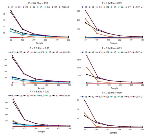
Figure 2. Relative efficiency of the estimators when C = 9.

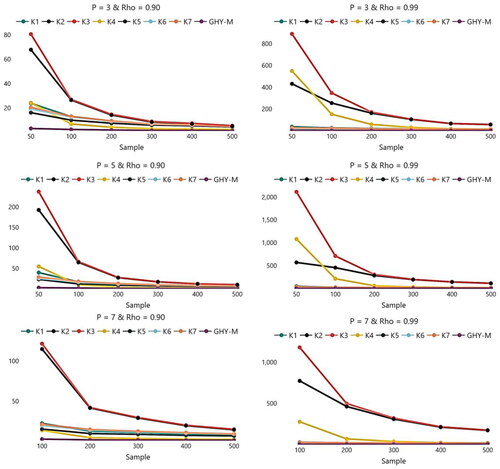
Table 1. MSE values of the estimators when $p =3$ and $C =5.$

		GLT-M
n	MLE	K1	K2	K3	K4	K5	K6	K7	GHY-M
$\rho =.90$
50	25.666	1.874	0.924	0.880	1.699	2.585	2.162	2.035	8.040
100	9.021	1.271	0.919	0.873	1.744	1.504	1.240	1.215	4.278
200	3.473	0.884	0.935	0.846	1.267	0.943	0.876	0.870	2.311
300	2.474	0.789	0.927	0.819	1.056	0.818	0.789	0.788	1.839
400	1.979	0.747	0.936	0.814	0.915	0.752	0.741	0.743	1.720
500	1.451	0.695	0.940	0.800	0.753	0.681	0.688	0.695	1.432
$\rho =.95$
50	30.713	2.428	0.949	0.914	1.850	3.266	2.417	2.295	11.893
100	16.930	1.721	0.911	0.884	1.869	2.320	1.846	1.769	6.902
200	7.177	1.168	0.913	0.859	1.653	1.373	1.146	1.121	3.907
300	4.788	0.982	0.923	0.854	1.489	1.127	1.013	0.999	3.006
400	3.594	0.902	0.927	0.843	1.270	0.984	0.892	0.884	2.740
500	3.112	0.844	0.928	0.837	1.190	0.908	0.843	0.838	2.646
$\rho =.99$
50	274.420	12.530	1.315	0.937	1.186	21.328	16.030	14.136	78.877
100	88.759	5.524	0.959	0.897	1.432	8.931	6.811	6.144	28.760
200	41.833	3.234	0.921	0.888	1.725	4.986	3.772	3.510	16.497
300	26.500	2.421	0.916	0.903	1.941	3.605	2.837	2.645	11.930
400	21.497	1.964	0.916	0.898	1.883	2.959	2.435	2.287	10.562
500	14.243	1.614	0.907	0.893	1.885	2.260	1.860	1.775	8.506

Table 2. MSE values of the estimators when $p =5$ and $C =5.$

		GLT-M
n	MLE	K1	K2	K3	K4	K5	K6	K7	GHY-M
$\rho =.90$
50	56.585	3.192	1.005	0.943	2.693	4.370	3.287	3.047	19.701
100	15.752	1.703	0.952	0.941	2.989	2.101	1.572	1.533	7.584
200	7.712	1.275	0.958	0.927	2.471	1.458	1.132	1.120	4.596
300	4.778	1.041	0.960	0.908	1.937	1.128	0.952	0.948	3.317
400	3.451	0.906	0.962	0.904	1.558	0.961	0.861	0.861	2.620
500	2.641	0.842	0.968	0.888	1.288	0.865	0.795	0.797	2.296
$\rho =.95$
50	83.575	4.089	1.000	0.947	2.630	5.886	4.566	4.082	25.134
100	33.397	2.772	0.954	0.945	3.244	3.622	2.500	2.372	12.934
200	14.976	1.835	0.951	0.939	3.145	2.248	1.616	1.571	7.704
300	10.236	1.453	0.956	0.948	2.756	1.716	1.307	1.279	5.804
400	7.091	1.254	0.956	0.937	2.343	1.437	1.133	1.116	4.665
500	6.109	1.149	0.964	0.929	2.171	1.275	1.058	1.047	4.203
$\rho =.99$
50	469.189	20.240	1.393	0.958	1.614	29.455	20.741	17.226	138.902
100	178.588	11.092	1.069	0.968	2.403	15.675	10.331	8.899	57.473
200	84.282	6.494	0.975	0.967	3.120	9.033	5.593	4.993	30.375
300	49.625	4.458	0.959	0.975	3.405	6.078	3.754	3.457	21.018
400	35.438	3.425	0.963	0.974	3.417	4.609	2.940	2.736	16.289
500	32.222	3.090	0.954	0.975	3.409	4.202	2.758	2.576	15.471

Table 3. MSE values of the estimators when $p =7$ and $C =5.$

		GLT-M
n	MLE	K1	K2	K3	K4	K5	K6	K7	GHY-M
$\rho =.90$
50	109.260	3.734	1.022	0.965	3.265	5.813	4.788	4.424	33.419
100	25.689	2.370	0.965	0.951	4.469	2.971	2.005	1.943	12.047
200	10.618	1.498	0.964	0.940	3.497	1.746	1.276	1.261	6.372
300	6.377	1.187	0.973	0.943	2.620	1.324	1.058	1.053	4.398
400	5.472	1.137	0.975	0.944	2.393	1.248	1.006	1.002	3.920
500	4.114	0.993	0.977	0.931	1.968	1.063	0.911	0.910	3.209
$\rho =.95$
50	189.602	7.451	1.100	0.973	3.051	11.023	8.419	7.446	58.543
100	55.651	3.983	0.983	0.961	4.461	5.192	3.464	3.193	20.167
200	24.974	2.400	0.970	0.965	4.482	2.973	2.052	1.955	11.049
300	14.695	1.868	0.973	0.972	3.969	2.222	1.533	1.494	8.159
400	11.115	1.588	0.973	0.977	3.542	1.840	1.325	1.302	6.653
500	8.239	1.409	0.972	0.965	3.031	1.600	1.178	1.166	5.662
$\rho =.99$
50	887.032	29.585	1.552	0.978	1.808	46.169	34.715	28.422	234.569
100	357.895	20.520	1.055	0.969	2.952	29.883	18.646	16.237	110.562
200	128.465	9.726	1.005	0.984	4.435	13.158	7.772	6.869	44.354
300	80.085	7.044	0.985	0.995	4.881	9.442	5.317	4.887	32.688
400	60.968	5.746	0.976	0.989	5.043	7.517	4.302	3.967	26.464
500	48.619	4.478	0.972	0.999	4.983	5.976	3.612	3.348	21.847

For all simulation situations, it can be noted that SMSE values of GLT-M and GHY-M estimators are less than SMSE values of MLE. This means that theses estimators have better performance than MLE for different cases of $n, \rho , p,$ and $C.$ Moreover, all the estimators have monotonic behaviors according to SMSE values. Namely, when the sample size $n$ increases, the estimated SMSE values decrease. It is obvious from tables and figures that by increasing the sample size affect positively on the performance of all estimators (including MLE). Also, it can be noted that, when $p$ and $\rho$ are fixed, increasing $C$ causes an increase in SMSE values of all estimators without exception. This increase is much larger in MLE than other estimators. Furthermore, when $C$ and $p$ are fixed, increasing $\rho$ affects SMSE values of all estimators negatively, especially MLE. In other words, this increase is much larger in MLE than other estimators. Also, increasing $p$ and $\rho$ with small $n$ inflates SMSE values of all estimators.

As expected, in the case of high multicollinearity, GLT-M and GHY-M estimators showed its best performance by means of the reduction of SMSE values and it is not affected by multicollinearity. But we note that GLT-M estimator for ${k1}_{hj},$ …, ${k7}_{hj}$ is better than GHY-M estimator in all simulation situations. And there is some difference between the performances of GLT-M estimators according to the shrinkage parameter $k$ that is used. According to our simulation study, it may be concluded that $K3$ is the best shrinkage parameter among others in most simulation situations.

5. Application

To illustrate the empirical relevance of the proposed estimators, we analyze Swedish football data in this empirical section. The proposed and existing estimators are elucidated using a dataset regarding the performance of Swedish football teams in the top Swedish league (Allsvenskan) during the year of 2018.¹

This dataset includes 242 observations and include one dependent variable (Y) is the full time results (H = Home win, D = Draw, A = Away win) of the football team, and nine explanatory variables, which are the pinnacle home win odds (PH), pinnacle draw odds (PD), pinnacle away win odds (PA), maximum Oddsportal home win odds (MaxH), maximum Oddsportal draw win odds (MaxD), maximum Oddsportal away win odds (MaxA), AvgH = average Oddsportal home win odds (AvgH), average Oddsportal draw win odds (AvgD), and average Oddsportal away win odds (AvgA). The effect of these regressors on Y, respectively are demonstrated by the A MNLR analysis.

The variance inflation factor (VIF) values of all explanatory variables are given in Table 4. From Table 4, it appears that the model is suffering from the multicollinearity problem as all VIFs are greater than 10. Also, the values of correlation coefficients between the explanatory variables are greater than 0.85 (in most of the cases). Table 5 presents estimates and standard errors (SE) values of MLE, GLT-M and GHY-M estimators. Table 5 indicates that GLT-M and GHY-M estimates have smaller SE values than MLE estimates. This means that GLT-M and GHY-M are efficient than MLE. These results are consistent with the simulation results in Sec. 4.

Table 4. Person correlation matrix of explanatory variables and VIF.

	PH	PD	PA	MaxH	MaxD	MaxA	AvgH	AvgD	AvgA
PH	1	−0.049	−0.575	0.997	−0.05	−0.555	0.995	−0.043	−0.589
PD	−0.049	1	0.756	−0.037	0.988	0.779	−0.064	0.989	0.766
PA	−0.575	0.756	1	−0.568	0.776	0.994	−0.595	0.773	0.995
MaxH	0.997	−0.037	−0.568	1	−0.04	−0.549	0.997	−0.033	−0.582
MaxD	−0.05	0.988	0.776	−0.04	1	0.8	−0.069	0.997	0.785
MaxA	−0.555	0.779	0.994	−0.549	0.8	1	−0.575	0.796	0.996
AvgH	0.995	−0.064	−0.595	0.997	−0.069	−0.575	1	−0.062	−0.609
AvgD	−0.043	0.989	0.773	−0.033	0.997	0.796	−0.062	1	0.781
AvgA	−0.589	0.766	0.995	−0.582	0.785	0.996	−0.609	0.781	1
VIF	767	2299	974	1655	7612	589	1480	9735	1514

Table 5. Parameter estimates and standard errors of MNLR model.

		GLT-M
Variable	MLE	K1	K2	K3	K4	K5	K6	K7	GHY-M
Estimate values: Level (A)
PH	0.3025	−0.0005	6.4E-06	0.0352	0.0004	0.1274	0.1279	0.1279	0.1845
PD	−1.5679	−0.0011	6.0E-05	0.0673	0.0007	−0.7383	−0.7528	−0.7523	−0.8659
PA	0.7867	−0.0002	2.8E-05	−0.0511	−0.0008	0.3672	0.3747	0.3759	0.3597
MaxH	−1.5223	−0.0009	9.8E-06	0.0024	3.1E-05	−0.2007	−0.1999	−0.1998	−1.1891
MaxD	7.0585	0.0002	1.5E-06	1.9E-05	2.1E-07	0.0243	0.0239	0.0239	3.4219
MaxA	−0.3697	−0.0631	0.0004	−0.0126	−0.0002	−0.2650	−0.1509	−0.1347	−0.2808
AvgH	1.2102	−0.0472	0.0030	0.0065	8.2E-05	0.2807	0.3132	0.3293	1.1188
AvgD	−5.0289	0.5102	0.0097	0.0044	4.7E-05	0.8248	−1.5435	−1.4598	−2.2152
AvgA	−1.1104	−0.3085	0.0007	−0.0008	−1.2E-05	−0.2507	−0.1476	−0.1244	−0.5236
Estimate values: Level (H)
PH	0.6125	−0.0887	−0.0042	−0.0008	−1.1E-06	0.0132	0.1094	0.0885	0.3795
PD	1.1539	0.8502	−0.0133	0.0139	0.0002	0.2813	0.4165	0.2816	0.8281
PA	0.1480	−0.0860	0.0023	0.0070	0.0001	0.0014	0.0244	0.0141	−0.0047
MaxH	−0.2835	−0.0477	−0.0023	−0.0002	−3.5E-07	−0.0741	−0.0161	−0.0272	−0.5154
MaxD	3.8905	−0.6169	−0.0084	0.0033	5.8E-05	−0.1007	0.7564	0.6731	1.5677
MaxA	−0.9426	−0.7505	0.0065	0.0077	0.0001	−0.8559	−0.1934	−0.2195	−0.8714
AvgH	−0.6379	−0.0033	−2.6E-05	−7.9E-07	1.5E-10	−0.0022	−0.0002	−0.0003	−0.0003
AvgD	−5.1105	−0.3153	−0.0019	0.0004	6.3E-06	−0.4193	−0.1821	−0.2005	−2.5389
AvgA	1.0343	1.2422	0.1372	0.0294	0.0005	1.3384	0.1523	−0.6598	1.2403
SE values: Level (A)
PH	1.1909	0.0008	1.4E-06	0.0070	0.0001	0.5026	0.5033	0.5033	0.5943
PD	1.9110	0.0051	1.8E-05	0.0170	0.0006	0.9158	0.9175	0.9175	1.3245
PA	1.1477	0.0197	5.1E-05	0.0165	0.0005	0.5418	0.5466	0.5463	0.5609
MaxH	1.6703	0.0011	2.1E-06	0.0005	8.7E-06	0.2207	0.2193	0.2193	0.8034
MaxD	3.3418	0.0001	4.5E-07	4.9E-06	1.8E-07	0.0115	0.0113	0.0113	2.8917
MaxA	0.8504	0.1664	0.0007	0.0041	0.0001	0.3657	0.3486	0.3449	0.3608
AvgH	1.7525	0.1670	0.0006	0.0013	2.4E-05	0.4775	0.4528	0.4543	0.8335
AvgD	4.0154	0.2717	0.0029	0.0011	3.9E-05	1.0044	1.2338	1.2047	4.9866
AvgA	1.5445	0.1948	0.0010	0.0003	9.1E-06	0.5010	0.2070	0.2148	0.8011
SE values: Level (H)
PH	1.9228	0.2206	0.0012	0.0008	1.1E-05	0.3218	0.3471	0.3449	1.2140
PD	1.7378	0.7888	0.0058	0.0047	0.0001	0.8207	0.6433	0.6243	1.7003
PA	0.6351	0.4692	0.0006	0.0014	0.0000	0.4412	0.1203	0.1227	0.2807
MaxH	2.2131	0.1767	0.0006	0.0002	2.4E-06	0.2481	0.1213	0.1223	1.2650
MaxD	3.0459	0.7417	0.0035	0.0011	1.9E-05	0.7881	0.5954	0.5688	3.0489
MaxA	0.5647	0.4319	0.0022	0.0016	0.0000	0.4301	0.1124	0.1247	0.2171
AvgH	2.1516	0.0032	7.12E-06	8.74E-07	1.2E-08	0.0030	0.0007	0.0007	1.1009
AvgD	3.7128	0.2628	0.0008	0.0001	2.1E-06	0.3100	0.1318	0.1388	4.3214
AvgA	1.1545	0.8203	0.0250	0.0057	0.0001	0.7938	0.3771	0.5398	0.7825

6. Some concluding remarks

To overcome the problem of multicollinearity, this paper proposes two generalized biased estimators for the multinomial logistic regression model by following the work of Abonazel and Farghali (2019), Farghali (2019), and Huang and Yang (2014). We discuss the MSE properties of the estimators and developed algorithms to estimate the biasing or shrinkage parameters $k_{hj}$ and $d_{hj}.$ A simulation study has been conducted to compare the performance of the estimators and to support the theoretical comparison. Simulation results indicated that increasing the correlation between the independent variables has a negative effect on the MSE, whereas, increasing the number of regressors and amount of correlation have a positive effect on MSE. When the sample size increases, the MSE values of the estimators decrease even when the correlation between regressors is large. It also appeared that proposed GLT-M performed better than both MLE and GHY-M estimator and GHY-M is doing better than MLE. Overall, the estimator based on K3 performed the best followed by K2, K1, and K4. For illustration purposes, Swedish football data are analyzed, which supported the simulation results and consistent with theoretical results of the paper. Finally, we recommend the researchers use the GLT-M estimator with parameter K3.

Notes

1 The data are publicly available on the webpage www.football-data.co.uk.

References

- Abonazel, M. R., and R. A. Farghali. 2019. Liu-type multinomial logistic estimator. Sankhya B 81 (2):203–25. doi: 10.1007/s13571-018-0171-4.
- Agresti, A. 2013. Categorical data analysis. 3rd ed. Hoboken, NJ: John Wiley& Sons, Inc.
- Akram, M. N., M. Amin, and M. Qasim. 2020. A new Liu-type estimator for the inverse Gaussian regression model. Journal of Statistical Computation and Simulation 90 (7):1153–72. doi: 10.1080/00949655.2020.1718150.
- Amin, M., M. Qasim, A. Yasin, and M. Amanullah. 2020a. Almost unbiased ridge estimator in the gamma regression model. Communications in Statistics-Simulation and Computation. Advance online publication. doi:10.1080/03610918.2020.1722837.
- Amin, M., M. Qasim, and M. Amanullah. 2019. Performance of Asar and Genç and Huang and Yang’s two-parameter estimation methods for the Gamma regression model. Iranian Journal of Science and Technology, Transactions A: Science 43 (6):2951–63. doi: 10.1007/s40995-019-00777-3.
- Amin, M., M. Qasim, M. Amanullah, and S. Afzal. 2020b. Performance of some ridge estimators for the gamma regression model. Statistical Papers 61 (3):997–1026. doi: 10.1007/s00362-017-0971-z.
- Asar, Y., and A. Genç. 2018. A new two-parameter estimator for the Poisson regression model. Iranian Journal of Science and Technology, Transactions A: Science 42 (2):793–803. doi: 10.1007/s40995-017-0174-4.
- Asl, M. N., H. Bevrani, R. A. Belaghi, and K. Mansson. 2021. Ridge-type shrinkage estimators in generalized linear models with an application to prostate cancer data. Statistical Papers 62 (2):1043–85. doi: 10.1007/s00362-019-01123-w.
- El-Dash, A., A. El-Hefnawy, and R. Farghali. 2011. Goal programming technique for correcting multicollinearity problem in multinomial logistic regression. The 46th Annual Conference on Statistics, Computer Sciences, and Operation Research, 26–29 Dec., 72–87.
- Farebrother, R. W. 1976. Further results on the mean square error of ridge regression. Journal of the Royal Statistical Society: Series B (Methodological) 38 (3):248–50. doi: 10.1111/j.2517-6161.1976.tb01588.x.
- Farghali, R. 2014. A suggested biased estimator for correcting multicollinearity in multinomial logistic regression. Egyptian Statistical Journal 58:183–97.
- Farghali, R. 2019. Generalized Liu-Type estimator for linear regression. International Journal of Research and Reviews and in Applied Sciences 38:52–63.
- Hoerl, A. E., and R. W. Kennard. 1970. Ridge regression: Biased estimation for nonorthogonal problems. Technometrics 12 (1):55–67. doi: 10.1080/00401706.1970.10488634.
- Hosmer, D., S. Lemeshow, and R. Sturdivant. 2013. Applied logistic regression. 3rd ed. New York: John Wiley& Sons, Inc.
- Huang, J., and H. Yang. 2014. A two-parameter estimator in the negative binomial regression model. Journal of Statistical Computation and Simulation 84 (1):124–34. doi: 10.1080/00949655.2012.696648.
- Karlsson, P., K. Månsson, and B. G. Kibria. 2020. A Liu estimator for the beta regression model and its application to chemical data. Journal of Chemometrics 34 (10):e3300. doi: 10.1002/cem.3300.
- Kejian, L. 1993. A new class of blased estimate in linear regression. Communications in Statistics - Theory and Methods 22 (2):393–402. doi: 10.1080/03610929308831027.
- Kibria, B. M. G. 2003. Performance of some new ridge regression estimators. Communications in Statistics - Simulation and Computation 32 (2):419–35. doi: 10.1081/SAC-120017499.
- Kurtoğlu, F., and M. R. Özkale. 2016. Liu estimation in generalized linear models: Application on gamma distributed response variable. Statistical Papers 57 (4):911–28. doi: 10.1007/s00362-016-0814-3.
- Luce, R. D. 1959. Individual choice behaviour: A theoretical analysis. New York: Wiley.
- Lukman, A. F., B. Aladeitan, K. Ayinde, and M. R. Abonazel. 2021. Modified ridge-type for the Poisson regression model: Simulation and application. Journal of Applied Statistics. Advance online publication. doi:10.1080/02664763.2021.1889998.
- Lukman, A. F., K. Ayinde, B. G. Kibria, and E. T. Adewuyi. 2020. Modified ridge-type estimator for the gamma regression model. Communications in Statistics-Simulation and Computation. Advance online publication. doi:10.1080/03610918.2020.1752720.
- Mandal, S., R. Arabi Belaghi, A. Mahmoudi, and M. Aminnejad. 2019. Stein‐type shrinkage estimators in gamma regression model with application to prostate cancer data. Statistics in Medicine 38 (22):4310–22. doi: 10.1002/sim.8297.
- Månsson, K. 2012. On ridge estimators for the negative binomial regression model. Economic Modelling 29 (2):178–84. doi: 10.1016/j.econmod.2011.09.009.
- Månsson, K. 2013. Developing a Liu estimator for the negative binomial regression model: Method and application. Journal of Statistical Computation and Simulation 83 (9):1773–80. doi: 10.1080/00949655.2012.673127.
- Månsson, K., and G. Shukur. 2011a. On ridge parameters in logistic regression. Communications in Statistics – Theory and Methods 40 (18):3366–81. doi: 10.1080/03610926.2010.500111.
- Månsson, K., and G. Shukur. 2011b. A Poisson ridge regression estimator. Economic Modelling 28 (4):1475–81. doi: 10.1016/j.econmod.2011.02.030.
- Månsson, K., B. M. G. Kibria, and G. Shukur. 2012. On Liu estimators for the logit regression model. Economic Modelling 29 (4):1483–8. doi: 10.1016/j.econmod.2011.11.015.
- Månsson, K., B. M. G. Shukur, and B. G. Kibria. 2018. Performance of some ridge regression estimators for the multinomial logit model. Communications in Statistics - Theory and Methods 47 (12):2795–804. doi: 10.1080/03610926.2013.784996.
- Månsson, K., G. Shukur, and B. M. G. Kibria. 2018. Performance of some ridge regression estimators for the multinomial logit model. Communications in Statistics - Theory and Methods 47 (12):2795–804. doi: 10.1080/03610926.2013.784996.
- Naveed, K., M. Amin, S. Afzal, and M. Qasim. 2020. New shrinkage parameters for the inverse Gaussian Liu regression. Communications in Statistics – Theory and Methods. Advance online publication. doi:10.1080/03610926.2020.1791339.
- Noori Asl, M., H. Bevrani, and R. Arabi Belaghi. 2020. Penalized and ridge-type shrinkage estimators in Poisson regression model. Communications in Statistics – Simulation and Computation. Advance online publication. doi:10.1080/03610918.2020.1730402.
- Özkale, M. R., and S. Kaciranlar. 2007. The restricted and unrestricted two-parameter estimators. Communications in Statistics – Theory and Methods —Theory and Methods, 36 (15):2707–25. doi: 10.1080/03610920701386877.
- Qasim, M., B. M. G. Kibria, K. Månsson, and P. Sjölander. 2020a. A new Poisson Liu regression estimator: Method and application. Journal of Applied Statistics 47 (12):2258–71. doi: 10.1080/02664763.2019.1707485.
- Qasim, M., K. Månsson, and B. M. Golam Kibria. 2021. On some beta ridge regression estimators: Method, simulation and application. Journal of Statistical Computation and Simulation. Advance online publication. doi:10.1080/00949655.2020.1867549.
- Qasim, M., K. Månsson, M. Amin, B. M. G. Kibria, and P. Sjölander. 2020b. Biased adjusted Poisson ridge estimators-method and application. Iranian Journal of Science and Technology, Transactions A: Science 44 (6):1775–89. doi: 10.1007/s40995-020-00974-5.
- Qasim, M., M. Amin, and M. Amanullah. 2018. On the performance of some new Liu parameters for the gamma regression model. Journal of Statistical Computation and Simulation 88 (16):3065–80. doi: 10.1080/00949655.2018.1498502.
- Rady, E. A., M. R. Abonazel, and I. M. Taha. 2019. New shrinkage parameters for liu-type zero inflated negative binomial estimator. The 54th Annual Conference on Statistics, Computer Science, and Operation Research 3-5 Dec, 2019. FGSSR, Cairo University.
- Schaefer, R. 1986. Alternative estimators in logistic regression when the data are collinear. Journal of Statistical Computation and Simulation 25 (1/2):75–91. doi: 10.1080/00949658608810925.
- Schaefer, R., L. Roi, and R. Wolfe. 1984. A ridge logistic estimator. Communications in Statistics - Theory and Methods 13 (1):99–113. doi: 10.1080/03610928408828664.
- Segerstedt, B. 1992. On ordinary ridge regression in generalized linear models. Communications in Statistics - Theory and Methods 21 (8):2227–46. doi: 10.1080/03610929208830909.
- Toker, S., G. Üstündağ Şiray, and M. Qasim. 2019. Developing a first order two parameter estimator for generalized linear model. Paper presented at the 11th International Statistics Congress; Muğla, Turkey.
- Trenkler, G., and H. Toutenburg. 1990. Mean squared error matrix comparisons between biased estimators—an overview of recent results. Statistical Papers 31 (1):165–79. doi: 10.1007/BF02924687.
- Yang, H., and X. Chang. 2010. A new two-parameter estimator in linear regression. Communications in Statistics – Theory and Methods 39 (6):923–34. doi: 10.1080/03610920902807911.