Multiple imputation regression discontinuity designs: Alternative to regression discontinuity designs to estimate the local average treatment effect at the cutoff

Abstract

The regression discontinuity design (RDD) is one of the most credible methods for causal inference that is often regarded as a missing data problem in the potential outcomes framework. However, the methods for missing data such as multiple imputation are rarely used as a method for causal inference. This article proposes multiple imputation regression discontinuity designs (MIRDDs), an alternative way of estimating the local average treatment effect at the cutoff point by multiply-imputing potential outcomes. To assess the performance of the proposed method, Monte Carlo simulations are conducted under 112 different settings, each repeated 5,000 times. The simulation results show that MIRDDs perform well in terms of bias, root mean squared error, coverage, and interval length compared to the standard RDD method. Also, additional simulations exhibit promising results compared to the state-of-the-art RDD methods. Finally, this article proposes to use MIRDDs as a graphical diagnostic tool for RDDs. We illustrate the proposed method with data on the incumbency advantage in U.S. House elections. To implement the proposed method, an easy-to-use software program is also provided.

Keywords:

• Causal inference
• Missing data
• Multiple imputation
• Potential outcome
• Regression discontinuity

1. Introduction

Causal inference has been established as a missing data problem using the potential outcomes framework (Rubin 1974, p. 689) due to the fundamental problem of causal inference (Holland 1986, p. 947). Among the many causal inference techniques for non-experimental data, the regression discontinuity design (RDD) is considered one of the strongest quasi-experimental designs, because RDDs allow us to achieve local randomization around the cutoff point (Lee and Lemieux 2015, p. 304; Kim and Steiner 2016). The recent literature on RDDs is also based on the potential outcomes framework (Lee 2008, p. 678; Imbens and Kalyanaraman 2012, p. 934; Calonico, Cattaneo, and Titiunik 2014, p. 2298).

In a related vein, Rubin (1987) proposed multiple imputation as a method of dealing with missing data. It is even said, “Multiple imputation is now accepted as the best general method to deal with incomplete data in many fields” (van Buuren 2018, p. 30). In both of the literatures of causal inference and missing data analysis, Rubin (1974, 1987) played an important role. Indeed, Rubin (2004, pp. 167–168) mentions the possibility of multiply-imputing missing potential outcomes, and recently, some suggestions have been made to use multiple imputation as a method of causal inference (Imbens and Rubin 2015, pp. 150–171; van Buuren 2018, pp. 241–255). As of today, however, little is known about the performance of multiple imputation to estimate the local average treatment effect (LATE) around the cutoff point.

This article proposes a novel application of multiple imputation for causal inference, which is named multiple imputation regression discontinuity designs (MIRDDs) to be used to estimate the LATE at the cutoff point. Monte Carlo simulations are conducted under 112 different settings, each repeated 5,000 times, and the results of the simulations show that MIRDDs perform well in terms of bias, root mean squared error, coverage, and interval length in comparison with the standard RDD method. Also, additional simulations exhibit promising results compared to the state-of-the-art RDD methods by Calonico, Cattaneo, and Titiunik (2014) and Branson et al. (2019).

Based on the findings that MIRDDs can be used to estimate the LATE at the cutoff, this article further presents a graphical method based on MIRDDs to diagnose the validity of RDD analyses. As Imbens and Lemieux (2008, p. 622) note, graphical analyses are an integral part of RDDs. Therefore, this article will be an important addition to the literature of RDDs in particular and of causal inference in general. We empirically illustrate the proposed method, replicating the renowned application of RDDs to the incumbency advantage in U.S. House elections by Lee (2008).

By way of organization, Sec. 2 reviews the potential outcomes framework that is often used in the causal inference literature, briefly explains how regression discontinuity designs work, and briefly introduces multiple imputation. Section 3 presents MIRDDs, where multiple imputation is used to estimate the LATE at the cutoff point. Section 4 presents Monte Carlo evidence. Section 5 suggests how MIRDDs can be used as a graphical diagnostic tool for RDDs, with an example on the incumbency advantage in U.S. House elections. Section 6 concludes. An easy-to-use software program is also provided in the Appendix.

2. Preliminary concepts in the existing frameworks and methods

This section briefly introduces the framework for causal inference and the mechanism of RDD and MI.

2.1. Review of the potential outcomes framework for causal inference

The modern literature on causal inference has been framed in the Rubin Causal Model, which regards causal inference as a problem of missing data using the concept of potential outcomes (Holland and Rubin 1988; Winship and Morgan 1999; Little and Rubin 2000).

The current study focuses on the causal effect of a binary intervention, which is called a treatment. Let $T_i$ be a treatment for individual $i,$ $T_i\in \left\{0,\mathrm{ }1\right\},$ where $T_i=0$ means that individuals are not exposed to the treatment while $T_i=1$ means that individuals are exposed to the treatment. Also, let $Y_i$ be a continuous outcome variable. The current study focuses on a continuous outcome variable, because the regression discontinuity design is based on a multiple regression model $Y_i={\beta }_0+{\beta }_1{X}_i+{\beta }_2{T}_i+{\epsilon }_i$ (Angrist and Pischke 2009, p. 253). We will explain $X_i$ later. Furthermore, let $Y_i\left(0\right)$ and $Y_i\left(1\right)$ denote the pair of potential outcomes for individual $i,$ where $Y_i\left(0\right)$ is the outcome without the treatment and $Y_i\left(1\right)$ is the outcome with the treatment. Then, the outcome we observe is Eq. (1)(1) $$Y_i=\left(1-T_i\right)Y_i\left(0\right)+T_i{Y}_i\left(1\right)=\{\begin{array}{cc}{Y}_i\left(0\right)& \text{if }{T}_i=0\\ Y_i\left(1\right)& \text{if }{T}_i=1\end{array}$$(1) (Imbens and Lemieux 2008, p. 616). (1) $$Y_i=\left(1-T_i\right)Y_i\left(0\right)+T_i{Y}_i\left(1\right)=\{\begin{array}{cc}{Y}_i\left(0\right)& \text{if }{T}_i=0\\ Y_i\left(1\right)& \text{if }{T}_i=1\end{array}$$(1)

The individual causal effect (or individual treatment effect) is $Y_i\left(1\right)-Y_i\left(0\right),$ which is the ultimate interest in causal inference. However, this quantity is unknown, because we only observe $Y_i\left(0\right)$ or $Y_i\left(1\right)$ for individual $i.$ This fact is known to be the “fundamental problem of causal inference” (Holland 1986, p. 947). Thus, we usually focus on the average causal effect (or average treatment effect: ATE) as in Eq. (2)(2) $$E\left[Y_i\left(1\right)-Y_i\left(0\right)\right]=E\left[Y_i\left(1\right)\right]-E\left[Y_i\left(0\right)\right]$$(2) that is “the effect on all individuals (treatment and control)” (Stuart 2010, p. 4). Equality in Eq. (2)(2) $$E\left[Y_i\left(1\right)-Y_i\left(0\right)\right]=E\left[Y_i\left(1\right)\right]-E\left[Y_i\left(0\right)\right]$$(2) follows from the property of expectation that the expectation of a sum is the sum of the expectations. (2) $$E\left[Y_i\left(1\right)-Y_i\left(0\right)\right]=E\left[Y_i\left(1\right)\right]-E\left[Y_i\left(0\right)\right]$$(2)

A naïve estimator takes the difference between the mean of observed $Y_i\left(1\right)$ and the mean of observed $Y_i\left(0\right).$ However, it could be confounded by some variables (observed and unobserved).

In the literature of missing data analysis, this naïve estimator is known as available-case analysis (also known as pairwise deletion) that is not a valid method unless data are missing completely at random (MCAR) (van Buuren 2018, p. 11; Little and Rubin 2020, pp. 61–62).

2.2. Overview of regression discontinuity designs

Let $X_i$ be a continuous variable that determines the assignment of $T_i.$ In the RDD literature, variable $X_i$ is called the forcing variable (Imbens and Kalyanaraman 2012, p. 934; Calonico, Cattaneo, and Titiunik 2014, p. 2298), the running variable (Branson et al. 2019, p. 15), or simply the assignment variable (Thoemmes, Liao, and Jin 2017, p. 341). The current study calls $X_i$ the forcing variable. In the sharp RDD, which is the focus in the current study, the assignment of a treatment is a deterministic function of $X_i$ as in Eq. (3)(3) $$T_i=\{\begin{array}{cc}1& \text{if }{X}_i\ge c\\ 0& \text{if }{X}_i<c\end{array}$$(3) , where $c$ is a cutoff point. (3) $$T_i=\{\begin{array}{cc}1& \text{if }{X}_i\ge c\\ 0& \text{if }{X}_i<c\end{array}$$(3)

Since $X_i$ deterministically assigns the treatment, $X_i$ is a confounder. This further means that there is no covariate overlap. Although the propensity score is one of the most often used techniques to address confounding, the propensity score cannot be used in this situation, due to the fact that the overlap assumption is essential for the propensity score (Imbens and Lemieux 2008, p. 618; Stuart 2010, p. 10; Imbens and Rubin 2015, p. 309).

Regression discontinuity designs (RDDs) may be able to address the problem identified above. An intuitive estimator is Eq. (4)(4) $$E\left[Y_i\left(1\right)|X_i=c\right]-E\left[Y_i\left(0\right)|X_i=c\right]$$(4) , where we take the difference of the expectations between the two groups exactly at the cutoff point. However, there are no observations exactly on the cutoff point. (4) $$E\left[Y_i\left(1\right)|X_i=c\right]-E\left[Y_i\left(0\right)|X_i=c\right]$$(4)

RDDs extend Analysis of Covariance (ANCOVA) as a valid method of causal inference by exploiting the fact that observations just above and below a cutoff can be thought of as a random subsample (Shadish, Cook, and Campbell 2002, p. 224). An intuitive explanation is that the difference in $X_i$ around the cutoff is in large part due to random noise. Suppose that $c=60.$ If math test scores for Students A and B are 59 and 60, respectively, then the true math ability of A and B is probably about the same within the margin of error, because no math tests can perfectly measure the true math ability, which further implies math test scores can be considered a function of ability + random noise. Nonetheless, Student A does not receive a treatment while Student B does. Thus, if we focus on a small enough neighborhood around the cutoff, the subsample can be considered a randomly assigned subgroup to the treatment, imitating the randomized experiment. Therefore, $X_i$ is the only confounding variable in RDDs, which is a remarkable characteristic of RDDs (Angrist and Pischke 2009, pp. 257–258). This is why, RDDs are said to be “stronger for causal inference than any design except the randomized experiment” (Shadish, Cook, and Campbell 2002, p. 221). Note that we will discuss the issue of bandwidth selection in Sec. 4.3.

The standard model that is used in an RDD is local linear regression, where we “fit linear regression functions to the observations within a distance $h$ on either side of the discontinuity point” (Imbens and Lemieux 2008, p. 624). This is known to be the local approach as opposed to the global approach such as ANCOVA (Thoemmes, Liao, and Jin 2017, p. 344). Indeed, Gelman and Imbens (2019, p. 448) argue that global high-order polynomial regressions should not be used for RDDs; instead, local low-order polynomials such as local linear or local quadratic models are more preferable. Which of the local linear or quadratic models is more appropriate in a given study may be diagnosed by the method presented in Sec. 5 of the current study.

Essentially, RDDs estimate the local average treatment effect (LATE) at the cutoff (Hahn, Todd, and Klaauw 2001, p. 204) as in Eq. (5)(5) $$\underset{x\downarrow c}{\lim }E\left[Y_i\left(1\right)|X_i=c\right]-\underset{x\uparrow c}{\lim }E\left[Y_i\left(0\right)|X_i=c\right]$$(5) , which further means that RDDs require the least amount of extrapolation to overcome the lack of covariate overlap (Branson et al. 2019, p. 15). (5) $$\underset{x\downarrow c}{\lim }E\left[Y_i\left(1\right)|X_i=c\right]-\underset{x\uparrow c}{\lim }E\left[Y_i\left(0\right)|X_i=c\right]$$(5)

Therefore, an RDD has an advantage that it avoids many complications about model specification, such as the selection of variables and functional forms (Hahn, Todd, and Klaauw 2001, p. 207).

2.3. Overview of multiple imputation

This section briefly introduces multiple imputation. For a more detailed account on multiple imputation, see Rubin (1987), King et al. (2001), Allison (2002, pp. 27–50), Enders (2010, pp. 164–253), and Carpenter and Kenward (2013).

When some observations are missing in a dataset, it is not possible to conduct statistical analyses. For example, when we have data (1, 3, 4, and NA), the arithmetic mean is (8 + NA)/4, which cannot be numerically computed. Imputation replaces a missing value by some plausible value, so that missing data become pseudo-complete data. For example, our imputed data may look like (1, 3, 4, and 2). Then, the arithmetic mean can be numerically computed as 2.5. However, imputed values are not observed values, but predicted values. This further means that there is uncertainty involved in imputed values. This fact needs to be accounted for in statistical analyses using imputed data.

In theory, multiple imputation replaces a missing value by $M$ values ($M>1$) independently and randomly drawn from the distribution of missing data. Uncertainty about missing data is reflected in the variation among these $M$ values. For example, our multiply-imputed data may look like (1, 3, 4, and 2), (1, 3, 4, and 0), and (1, 3, 4, and 3). In practice, however, we do not observe missing data by definition, which further means that we do not observe the distribution of missing data.

Under the assumption of missing at random (MAR), where the conditional probability of missing data after controlling for observed data is the same as the probability of observed data (King et al. 2001; Allison 2002, p. 4; Enders 2010, p. 11; Little and Rubin 2020, p. 14), multiple imputation constructs the posterior predictive distribution of missing data conditional on observed data. Then, multiple imputation independently and randomly draws $M$ simulated values from this posterior predictive distribution. Equation (3)(3) $$T_i=\{\begin{array}{cc}1& \text{if }{X}_i\ge c\\ 0& \text{if }{X}_i<c\end{array}$$(3) states that $Y_i\left(0\right)$ is missing when $X_i\ge c$ and $Y_i\left(1\right)$ is missing when $X_i<c.$ Both of these are archetypical MAR. Therefore, it is natural to think that we can apply multiple imputation for the missing portion of $Y_i\left(0\right)$ and $Y_i\left(1\right).$ In other words, potential outcomes are missing at random in the sense of MAR in the RDD context.

However, it is difficult to randomly draw sufficient statistics from the posterior predictive distribution using the traditional analytical methods. In order to solve this problem, the following three computational algorithms have been proposed in the literature. The traditional algorithm of multiple imputation is the data augmentation (DA) algorithm, which is a Markov chain Monte Carlo (MCMC) technique. For the DA version of multiple imputation, see Schafer (1997, pp. 89–145). An alternative algorithm to DA is the fully conditional specification (FCS) algorithm, which specifies a multivariate distribution by way of a series of conditional densities, through which missing values are imputed given the other variables. Under the compatible conditional densities, FCS is a Gibbs sampler, a type of MCMC (van Buuren 2018, p. 120). For the FCS version of multiple imputation, see van Buuren (2018). Another alternative algorithm is the expectation-maximization with bootstrapping (EMB) algorithm, which combines the expectation-maximization (EM) algorithm with the nonparametric bootstrap to create multiply-imputed values of missing data. For the EMB version of multiple imputation, see Honaker and King (2010).

Takahashi (2017) finds that all of the three algorithms are valid methods of multiple imputation for continuous variables, that the EMB algorithm is the fastest among these algorithms, and that the EMB algorithm is most user-friendly. Thus, the analyses in this article are based on the EMB algorithm. Also, Little and Rubin (2020, p. 240) note, “the ML estimates from the bootstrap resamples are asymptotically equivalent to a sample from the posterior distribution of $\theta .$” Therefore, the EMB version of multiple imputation has the right properties to be used in place of MCMC algorithms (Honaker and King 2010, p. 565). The EMB version of multiple imputation is implemented in R-package Amelia (Honaker, King, and Blackwell 2011; Honaker, King, and Blackwell 2019).

Recently, some authors have contended that multiple imputation can be used as a method of causal inference. For example, Dore et al. (2013, p. S45) suggested a method to impute the missing potential outcomes by combining multiple imputation with the propensity score. Westreich et al. (2015) illustrated the possibility of using multiple imputation as a method of causal inference. Gutman and Rubin (2013, 2015) proposed multiple imputation using two splines in subclasses (MITSS) as a procedure to address causal inference from a missing data perspective. Olszewski et al. (2017, p. 108) applied MITSS to immunochemotherapy regimens. Nilsson et al. (2019, p. 825) imputed potential outcomes for causal inference using single imputation. However, little is known about the possibility of using multiple imputation to estimate the LATE at the cutoff. This article fills this gap in the literature.

3. Multiple imputation as a method of estimating the LATE at the cutoff

This section presents multiple imputation regression discontinuity designs (MIRDDS). Following Imbens and Rubin (2015, pp. 150–171) and van Buuren (2018, p. 245), the imputations in Eqs. (6)(6) $$\tilde{Y}\left(1\right)\sim Pr\left[Y_{\mathit{miss}}\left(1\right)\left|Y_{\mathit{obs}}\right(1),Y(0),X,{\tilde{\theta }}_1\right]$$(6) and (7)(7) $$\tilde{Y}\left(0\right)\sim Pr\left[Y_{\mathit{miss}}\left(0\right)\left|Y_{\mathit{obs}}\right(0),Y(1),X,{\tilde{\theta }}_0\right]$$(7) are alternated to create multiply-imputed values of the missing potential outcomes, where ${\tilde{\theta }}_1$ and ${\tilde{\theta }}_0$ are draws from the parameters of the imputation models, ∼ indicates a random draw from the predictive posterior distribution, $Y_{\mathit{miss}}$ is the unobserved portion of $Y,$ and $Y_{\mathit{obs}}$ is the observed portion of $Y.$ (6) $$\tilde{Y}\left(1\right)\sim Pr\left[Y_{\mathit{miss}}\left(1\right)\left|Y_{\mathit{obs}}\right(1),Y(0),X,{\tilde{\theta }}_1\right]$$(6) (7) $$\tilde{Y}\left(0\right)\sim Pr\left[Y_{\mathit{miss}}\left(0\right)\left|Y_{\mathit{obs}}\right(0),Y(1),X,{\tilde{\theta }}_0\right]$$(7)

Since multiple imputation alternates Eqs. (6)(6) $$\tilde{Y}\left(1\right)\sim Pr\left[Y_{\mathit{miss}}\left(1\right)\left|Y_{\mathit{obs}}\right(1),Y(0),X,{\tilde{\theta }}_1\right]$$(6) and (7)(7) $$\tilde{Y}\left(0\right)\sim Pr\left[Y_{\mathit{miss}}\left(0\right)\left|Y_{\mathit{obs}}\right(0),Y(1),X,{\tilde{\theta }}_0\right]$$(7) , the different parameters of the imputation models are estimated for $\tilde{Y}\left(1\right)$ and $\tilde{Y}\left(0\right).$ This allows us to adequately estimate the causal impact when the assumption of homogeneity of regression is violated, meaning that $Y\left(1\right)$ and $Y\left(0\right)$ have different regression slopes. This is in line with the concept of local regression explained in Sec. 2.

Let $D$ be an $n\times p$ dataset, where $n$ is the number of observations and $p$ is the number of variables. In a basic setup, we have two potential outcomes and one forcing variable, i.e., $p=3$ and $D=\left\{X,\mathrm{ }Y\left(0\right),Y\left(1\right)\right\},$ but we may have additional covariates as well to increase efficiency. Just as in RDDs, the proposed method in the current study also uses dataset $D$ in a small enough neighborhood around the cutoff. In this section, for simplicity, we assume that $D$ is already narrowed down in a small enough neighborhood around the cutoff, $c\pm h,$ where $c$ is the cutoff point and $h$ is a distance from $c.$ For the selection of bandwidth $h,$ see Sec. 4.3.

The EMB algorithm works as follows (Honaker and King 2010, p. 565). Bootstrap resamples of size $n$ are randomly drawn from $D$ with replacement $M$ times (Horowitz 2001, pp. 3163–3165; Carsey and Harden 2014, p. 215). The variation among these $M$ resamples represents uncertainty about estimation of missing data. Since $D$ is incomplete, the bootstrap resamples are also incomplete. Therefore, the expectation-maximization (EM) algorithm is applied to each of these $M$ bootstrap resamples, which is an iterative method for maximum likelihood estimation (MLE) for incomplete data (Little and Rubin 2020, p. 187). In other words, the EM algorithm is used to refine $M$ point estimates of parameter $\theta$ in the imputation model. Specifically, the mean vector and the variance-covariance matrix are estimated by the EM algorithm as follows. Equation (8)(8) $$Q\left(\theta |{\theta }^{\left(t\right)}\right)=\int l\left(\theta |Y\right)Pr\left(Y_{\mathit{miss}}|Y_{\mathit{obs}},{\theta }^{\left(t\right)}\right)d{Y}_{\mathit{miss}}$$(8) is the expectation step that calculates the $Q$-function by averaging the complete-data log-likelihood $l\left(\theta |Y\right)$ over the predictive distribution of missing data, where ${\theta }^{(t)}$ is an estimate of the unknown parameter at iteration $t.$ Equation (9)(9) $${\theta }^{(t+1)}=\arg \underset{\theta }{\max }Q\left(\theta |{\theta }^{\left(t\right)}\right)$$(9) is the maximization step that finds parameter values at iteration $t+1$ by maximizing the $Q$-function (Schafer 1997, pp. 37–39). (8) $$Q\left(\theta |{\theta }^{\left(t\right)}\right)=\int l\left(\theta |Y\right)Pr\left(Y_{\mathit{miss}}|Y_{\mathit{obs}},{\theta }^{\left(t\right)}\right)d{Y}_{\mathit{miss}}$$(8) (9) $${\theta }^{(t+1)}=\arg \underset{\theta }{\max }Q\left(\theta |{\theta }^{\left(t\right)}\right)$$(9)

After obtaining the refined $M$ estimates of the mean vector and the variance-covariance matrix, we can calculate $M$ local linear regression imputation models as in Eqs. (10)(10) $$\{\begin{array}{c}{\tilde{Y}}_1\left(1\right)={\tilde{\theta }}_{0,1}+{\tilde{\theta }}_{1,1}{Y}_{\mathit{obs}}\left(1\right)+{\tilde{\theta }}_{2,1}Y\left(0\right)+{\tilde{\theta }}_{3,1}X+{\tilde{\epsilon }}_{i,11}\\ {\tilde{Y}}_2\left(1\right)={\tilde{\theta }}_{0,2}+{\tilde{\theta }}_{1,2}{Y}_{\mathit{obs}}\left(1\right)+{\tilde{\theta }}_{2,2}Y\left(0\right)+{\tilde{\theta }}_{3,2}X+{\tilde{\epsilon }}_{i,12}\\ {\tilde{Y}}_3\left(1\right)={\tilde{\theta }}_{0,3}+{\tilde{\theta }}_{1,3}{Y}_{\mathit{obs}}\left(1\right)+{\tilde{\theta }}_{2,3}Y\left(0\right)+{\tilde{\theta }}_{3,3}X+{\tilde{\epsilon }}_{i,13}\end{array}$$(10) and (11)(11) $$\{\begin{array}{c}{\tilde{Y}}_1\left(0\right)={\tilde{\theta }}_{0,1}^{\mathrm{*}}+{\tilde{\theta }}_{1,1}^{\mathrm{*}}{Y}_{\mathit{obs}}\left(0\right)+{\tilde{\theta }}_{2,1}^{\mathrm{*}}Y\left(1\right)+{\tilde{\theta }}_{3,1}^{\mathrm{*}}X+{\tilde{\epsilon }}_{i,01}\\ {\tilde{Y}}_2\left(0\right)={\tilde{\theta }}_{0,2}^{\mathrm{*}}+{\tilde{\theta }}_{1,2}^{\mathrm{*}}{Y}_{\mathit{obs}}\left(0\right)+{\tilde{\theta }}_{2,2}^{\mathrm{*}}Y\left(1\right)+{\tilde{\theta }}_{3,2}^{\mathrm{*}}X+{\tilde{\epsilon }}_{i,02}\\ {\tilde{Y}}_3\left(0\right)={\tilde{\theta }}_{0,3}^{\mathrm{*}}+{\tilde{\theta }}_{1,3}^{\mathrm{*}}{Y}_{\mathit{obs}}\left(0\right)+{\tilde{\theta }}_{2,3}^{\mathrm{*}}Y\left(1\right)+{\tilde{\theta }}_{3,3}^{\mathrm{*}}X+{\tilde{\epsilon }}_{i,03}\end{array}$$(11) , where $M=3$ in this case. Note that these models can be easily extended to a local quadratic model by including the square term of $X$ in the model. Estimation uncertainty is represented by $M$ regression equations, and fundamental uncertainty by ${\tilde{\epsilon }}_{i,1}\sim N\left(0,\mathrm{ }{\tilde{\sigma }}_1^2\right)$ and ${\tilde{\epsilon }}_{i,0}\sim N\left(0,\mathrm{ }{\tilde{\sigma }}_0^2\right)$ (King et al. 2001, p. 54; van Buuren 2018, p. 67). (10) $$\{\begin{array}{c}{\tilde{Y}}_1\left(1\right)={\tilde{\theta }}_{0,1}+{\tilde{\theta }}_{1,1}{Y}_{\mathit{obs}}\left(1\right)+{\tilde{\theta }}_{2,1}Y\left(0\right)+{\tilde{\theta }}_{3,1}X+{\tilde{\epsilon }}_{i,11}\\ {\tilde{Y}}_2\left(1\right)={\tilde{\theta }}_{0,2}+{\tilde{\theta }}_{1,2}{Y}_{\mathit{obs}}\left(1\right)+{\tilde{\theta }}_{2,2}Y\left(0\right)+{\tilde{\theta }}_{3,2}X+{\tilde{\epsilon }}_{i,12}\\ {\tilde{Y}}_3\left(1\right)={\tilde{\theta }}_{0,3}+{\tilde{\theta }}_{1,3}{Y}_{\mathit{obs}}\left(1\right)+{\tilde{\theta }}_{2,3}Y\left(0\right)+{\tilde{\theta }}_{3,3}X+{\tilde{\epsilon }}_{i,13}\end{array}$$(10) (11) $$\{\begin{array}{c}{\tilde{Y}}_1\left(0\right)={\tilde{\theta }}_{0,1}^{\mathrm{*}}+{\tilde{\theta }}_{1,1}^{\mathrm{*}}{Y}_{\mathit{obs}}\left(0\right)+{\tilde{\theta }}_{2,1}^{\mathrm{*}}Y\left(1\right)+{\tilde{\theta }}_{3,1}^{\mathrm{*}}X+{\tilde{\epsilon }}_{i,01}\\ {\tilde{Y}}_2\left(0\right)={\tilde{\theta }}_{0,2}^{\mathrm{*}}+{\tilde{\theta }}_{1,2}^{\mathrm{*}}{Y}_{\mathit{obs}}\left(0\right)+{\tilde{\theta }}_{2,2}^{\mathrm{*}}Y\left(1\right)+{\tilde{\theta }}_{3,2}^{\mathrm{*}}X+{\tilde{\epsilon }}_{i,02}\\ {\tilde{Y}}_3\left(0\right)={\tilde{\theta }}_{0,3}^{\mathrm{*}}+{\tilde{\theta }}_{1,3}^{\mathrm{*}}{Y}_{\mathit{obs}}\left(0\right)+{\tilde{\theta }}_{2,3}^{\mathrm{*}}Y\left(1\right)+{\tilde{\theta }}_{3,3}^{\mathrm{*}}X+{\tilde{\epsilon }}_{i,03}\end{array}$$(11)

After multiple imputation, analysis can proceed as if the data are complete, meaning that as if we observe potential outcomes. Let ${\widehat{\tau }}_m$ be a point estimate of the LATE based on the $m$-th multiply-imputed dataset as in Eq. (12)(12) $${\widehat{\tau }}_m=E\left[{\tilde{Y}}_m\left(1\right)|c-h\le X_i\le c+h\right]-E\left[{\tilde{Y}}_m\left(0\right)|c-h\le X_i\le c+h\right]$$(12) (12) $${\widehat{\tau }}_m=E\left[{\tilde{Y}}_m\left(1\right)|c-h\le X_i\le c+h\right]-E\left[{\tilde{Y}}_m\left(0\right)|c-h\le X_i\le c+h\right]$$(12)

The combined point estimate of the LATE at the cutoff can be calculated by pooling the $M$ results by Rubin’s rule (Rubin 1987, p. 76; King et al. 2001, p. 53; van Buuren 2018, pp. 42–43). The combined point estimate ${\overline{\tau }}_M$ is Eq. (13)(13) $${\overline{\tau }}_M=\frac{1}{M}\sum _{m=1}^M{\widehat{\tau }}_m$$(13) , which is simply an arithmetic mean of $M$ estimates. (13) $${\overline{\tau }}_M=\frac{1}{M}\sum _{m=1}^M{\widehat{\tau }}_m$$(13)

The variance of the combined point estimate can be also pooled by Rubin’s rule. Let $v_m$ be $\mathit{var}\left({\widehat{\tau }}_m\right)/n_{\mathit{sub}},$ where $n_{\mathit{sub}}$ is the subsample size in the area $c\hspace{0.17em}\pm \hspace{0.17em}h.$ ${\overline{W}}_M$ is the average of within-imputation variance as in Eq. (14)(14) $${\overline{W}}_M=\frac{1}{M}\sum _{m=1}^M{v}_m$$(14) , which is simply an arithmetic mean and represents the usual concept of sampling variability. ${\overline{B}}_M$ is the average of between-imputation variance as in Eq. (15)(15) $${\overline{B}}_M=\frac{1}{M-1}\sum _{m=1}^M{\left({\widehat{\tau }}_m-{\overline{\tau }}_M\right)}^2$$(15) , which captures the estimation uncertainty due to missing data. $T_M$ is the total, combined variance of ${\overline{\tau }}_M$ as in Eq. (16)(16) $$T_M={\overline{W}}_M+\left(1+\frac{1}{M}\right){\overline{B}}_M$$(16) , where $1+1/M$ adjusts for the fact that $M$ is finite (Enders 2010, pp. 222–223). The 95% confidence interval ($CI$) can be computed as in Eq. (17)(17) $${CI}_{95\mathrm{\%}}={\overline{\tau }}_M\pm t_{0.025}\left(n_{\mathit{sub}}-1\right)\sqrt{T_M}$$(17) , where $t_{0.025}\left(n_{\mathit{sub}}-1\right)$ is a t-value with the degrees of freedom $n_{\mathit{sub}}-1.$ This is just a paired $t$-test situation; thus, inference is straightforward. (14) $${\overline{W}}_M=\frac{1}{M}\sum _{m=1}^M{v}_m$$(14) (15) $${\overline{B}}_M=\frac{1}{M-1}\sum _{m=1}^M{\left({\widehat{\tau }}_m-{\overline{\tau }}_M\right)}^2$$(15) (16) $$T_M={\overline{W}}_M+\left(1+\frac{1}{M}\right){\overline{B}}_M$$(16) (17) $${CI}_{95\mathrm{\%}}={\overline{\tau }}_M\pm t_{0.025}\left(n_{\mathit{sub}}-1\right)\sqrt{T_M}$$(17)

4. Monte Carlo simulations

4.1. Settings of population data

We will conduct simulations based on seven different data generation processes to show that MIRDDs can indeed estimate the LATE at the cutoff point. Simulations are conducted in R version 4.0.2. In all of the seven designs, $Z$-values are generated by a Beta distribution with parameters $\mathrm{\alpha }=2$ and $\mathrm{\beta }=4,$ based on which the forcing variable is $X=2Z-1.$ Also, the error term is ${\epsilon }_i\sim N\left(0,\mathrm{ }{0.1295}^2\right).$ These settings are commonly used in the RDD literature (Imbens and Kalyanaraman 2012, p. 950; Calonico, Cattaneo, and Titiunik 2014, p. 2314; Branson et al. 2019, p20). Simulation runs are repeated 5,000 times for each data generation process just as in Imbens and Kalyanaraman (2012) and Calonico, Cattaneo, and Titiunik (2014). Designs 1 to 4 were first used in the simulations of Imbens and Kalyanaraman (2012), and subsequently used in Calonico, Cattaneo, and Titiunik (2014) and Branson et al. (2019). Designs 5 and 6 were first used in the simulations of Calonico, Cattaneo, and Titiunik (2014), and subsequently used in Branson et al. (2019). Design 7 was first used in Branson et al. (2019).

In design 1, the regression function is a fifth-order polynomial with different coefficients used for $X_i<\mathrm{c}$ and $X_i\ge \mathrm{c},$ where $\mathrm{c}$ is the cutoff point, as in Eq. (18)(18) $$\{\begin{array}{c}Y\left(0\right)=0.48+1.27x+7.18x^2+20.21x^3+21.54x^4+7.33x^5+{\epsilon }_i\\ Y\left(1\right)=0.52+0.84x-3.00x^2+7.99x^3-9.01x^4+3.56x^5+{\epsilon }_i\mathrm{ }\end{array}$$(18) . This setting is based on the study of the incumbency advantage in U.S. House elections by Lee (2008). (18) $$\{\begin{array}{c}Y\left(0\right)=0.48+1.27x+7.18x^2+20.21x^3+21.54x^4+7.33x^5+{\epsilon }_i\\ Y\left(1\right)=0.52+0.84x-3.00x^2+7.99x^3-9.01x^4+3.56x^5+{\epsilon }_i\mathrm{ }\end{array}$$(18)

In design 2, the regression function is quadratic with different coefficients used for $X_i<\mathrm{c}$ and $X_i\ge \mathrm{c}$ as in Eq. (19)(19) $$\{\begin{array}{c}Y\left(0\right)=3x^2+{\epsilon }_i\\ Y\left(1\right)=4x^2+{\epsilon }_i\end{array}$$(19) . (19) $$\{\begin{array}{c}Y\left(0\right)=3x^2+{\epsilon }_i\\ Y\left(1\right)=4x^2+{\epsilon }_i\end{array}$$(19)

In design 3, the regression function is a fifth-order polynomial with the same coefficients used for $X_i<\mathrm{c}$ and $X_i\ge \mathrm{c},$ but the intercept is different by 0.1 points, i.e., a constant average treatment effect, as in Eq. (20)(20) $$\{\begin{array}{c}Y\left(0\right)=0.42+0.84x-3.00x^2+7.99x^3-9.01x^4+3.56x^5+{\epsilon }_i\\ Y\left(1\right)=0.52+0.84x-3.00x^2+7.99x^3-9.01x^4+3.56x^5+{\epsilon }_i\end{array}$$(20) . (20) $$\{\begin{array}{c}Y\left(0\right)=0.42+0.84x-3.00x^2+7.99x^3-9.01x^4+3.56x^5+{\epsilon }_i\\ Y\left(1\right)=0.52+0.84x-3.00x^2+7.99x^3-9.01x^4+3.56x^5+{\epsilon }_i\end{array}$$(20)

In design 4, the regression function is a modification of the third design without $x^2$ as in Eq. (21)(21) $$\{\begin{array}{c}Y\left(0\right)=0.42+0.84x+7.99x^3-9.01x^4+3.56x^5+{\epsilon }_i\\ Y\left(1\right)=0.52+0.84x+7.99x^3-9.01x^4+3.56x^5+{\epsilon }_i\end{array}$$(21) . (21) $$\{\begin{array}{c}Y\left(0\right)=0.42+0.84x+7.99x^3-9.01x^4+3.56x^5+{\epsilon }_i\\ Y\left(1\right)=0.52+0.84x+7.99x^3-9.01x^4+3.56x^5+{\epsilon }_i\end{array}$$(21)

In design 5, the regression function is a fifth-order polynomial with different coefficients used for $X_i<\mathrm{c}$ and $X_i\ge \mathrm{c}$ as in Eq. (22)(22) $$\{\begin{array}{c}Y\left(0\right)=3.71+2.30x+3.28x^2+1.45x^3+0.23x^4+0.03x^5+{\epsilon }_i\mathrm{ }\\ Y\left(1\right)=0.26+18.49x-54.81x^2+74.30x^3-45.02x^4+9.83x^5+{\epsilon }_i\end{array}$$(22) . This setting is based on the study on Head Start funding by Ludwig and Miller (2007). (22) $$\{\begin{array}{c}Y\left(0\right)=3.71+2.30x+3.28x^2+1.45x^3+0.23x^4+0.03x^5+{\epsilon }_i\mathrm{ }\\ Y\left(1\right)=0.26+18.49x-54.81x^2+74.30x^3-45.02x^4+9.83x^5+{\epsilon }_i\end{array}$$(22)

In design 6, the regression function is a modification of design 1 with coefficients multiplied by constants in bold-faces to increase curvature as in Eq. (23)(23) $$\{\begin{array}{c}\begin{array}{c}Y\left(0\right)=0.48+1.27x+\mathbf{0}\mathbf{.}\mathbf{5}\times 7.18x^2+\mathbf{0}\mathbf{.}\mathbf{7}\times 20.21x^3+\mathbf{1}\mathbf{.}\mathbf{1}\times 21.54x^4\\ +\mathbf{1}\mathbf{.}\mathbf{5}\times 7.33x^5+{\epsilon }_i\end{array}\\ Y\left(1\right)=0.52+0.84x-\mathbf{0}\mathbf{.}\mathbf{1}\times 3.00x^2-\mathbf{0}\mathbf{.}\mathbf{3}\times 7.99x^3-\mathbf{0}\mathbf{.}\mathbf{1}\times 9.01x^4 \\ +3.56x^5+{\epsilon }_i\end{array}$$(23) . (23) $$\{\begin{array}{c}\begin{array}{c}Y\left(0\right)=0.48+1.27x+\mathbf{0}\mathbf{.}\mathbf{5}\times 7.18x^2+\mathbf{0}\mathbf{.}\mathbf{7}\times 20.21x^3+\mathbf{1}\mathbf{.}\mathbf{1}\times 21.54x^4\\ +\mathbf{1}\mathbf{.}\mathbf{5}\times 7.33x^5+{\epsilon }_i\end{array}\\ Y\left(1\right)=0.52+0.84x-\mathbf{0}\mathbf{.}\mathbf{1}\times 3.00x^2-\mathbf{0}\mathbf{.}\mathbf{3}\times 7.99x^3-\mathbf{0}\mathbf{.}\mathbf{1}\times 9.01x^4 \\ +3.56x^5+{\epsilon }_i\end{array}$$(23)

In design 7, the regression function is cubic with different coefficients used for $X_i<\mathrm{c}$ and $X_i\ge \mathrm{c}$ as in Eq. (24)(24) $$\{\begin{array}{c}Y\left(0\right)=3x^3+{\epsilon }_i\\ Y\left(1\right)=4x^3+{\epsilon }_i\end{array}$$(24) . (24) $$\{\begin{array}{c}Y\left(0\right)=3x^3+{\epsilon }_i\\ Y\left(1\right)=4x^3+{\epsilon }_i\end{array}$$(24)

4.2. Settings of the sample size

While the sample size was set to 500 in Imbens and Kalyanaraman (2012), Calonico, Cattaneo, and Titiunik (2014), and Branson et al. (2019), the sample size in the current study is set to 6,558. This larger sample size is chosen for the following reasons. It is well-known that an RDD generally needs more observations than the standard statistical analyses because using a small neighborhood of the cutoff means that there is not much data (Shadish, Cook, and Campbell 2002, p. 212; Angrist and Pischke 2009, p. 256). In fact, Lee (2008, p. 691) used the sample size of 6,558, which is the widely cited paper as an exemplar of RDDs. Therefore, in line with the sample size used in Lee (2008), the current study sets the sample size to 6,558, because this is a more realistic sample size for RDDs. Results based on the sample size of 500 are also reported in Sec. 4.8.

4.3. Settings of bandwidths

A bandwidth is calculated by an MSE-optimal bandwidth selector for the difference of regression estimates (mserd), using R-function rdbwselect in R-package rdrobust (Calonico, Cattaneo, and Titiunik 2014, p. 2309; Calonico, Cattaneo, and Titiunik 2020, p. 4), where MSE stands for the Mean Squared Error. R-package rdrobust is known to be the most advanced RDD package in R, especially for the choice of bandwidth (Thoemmes, Liao, and Jin 2017, p. 349). Section 4.7 reports the results based on this bandwidth selector.

We also use other bandwidth estimation methods: An MSE-optimal bandwidth selector for the sum of regression estimates (msesum), a CER-optimal bandwidth selector for the difference of regression estimates (cerrd), and a CER-optimal bandwidth selector for the sum of regression estimates (cersum), where CER stands for the Coverage Error Rate (Calonico, Cattaneo, and Titiunik 2020, p. 4). The results for these are reported in the Online Appendix A.

Imbens and Lemieux (2008, p. 633) advise that we should always explore the sensitivity to the choice of bandwidths by using larger or smaller bandwidths than the originally chosen size. Therefore, we also use the bandwidths twice and half of the default size.

4.4. Settings of cutoff points

The cutoff point in Imbens and Kalyanaraman (2012), Calonico, Cattaneo, and Titiunik (2014), and Branson et al. (2019) is all set to $\mathrm{c}=0.$ However, the performance of RDDs depends on the location of the cutoff point (Shadish, Cook, and Campbell 2002, p. 217). Therefore, we also include other cutoff points at $\mathrm{c}=Q_1\left(x\right),$ $\mathrm{c}=Q_2\left(x\right),$ and $\mathrm{c}=Q_3\left(x\right),$ where $Q_1$ is the first quartile, $Q_2$ is the median, and $Q_3$ is the third quartile. Section 4.7 reports the results based on $\mathrm{c}=Q_2\left(x\right),$ because the results by RDDs are most powerful when the cutoff point is around the center of the distribution of the forcing variable (Shadish, Cook, and Campbell 2002, p. 217). Results based on the other cutoff points are reported in the Online Appendix A.

4.5. Evaluation criteria for the simulations

Let $\tau$ be the true population parameter and $\widehat{\tau }$ be an estimator of $\tau .$ If $\mathrm{Bias}\left(\widehat{\tau }\right)=0$ in Eq. (25)(25) $$\mathrm{Bias}\left(\widehat{\tau }\right)=E\left(\widehat{\tau }\right)-\tau$$(25) , the expected value of $\widehat{\tau }$ is equal to the true $\tau .$ Then, this estimator $\widehat{\tau }$ is an unbiased estimator of true parameter $\tau$ (Mooney 1997, p. 59; Gujarati 2003, p. 899). Therefore, a good estimator has bias closer to zero. (25) $$\mathrm{Bias}\left(\widehat{\tau }\right)=E\left(\widehat{\tau }\right)-\tau$$(25)

Under some circumstances, however, there is a tradeoff between bias and efficiency of two estimators, because one estimator may have larger bias, but may have smaller variance than another estimator. A slightly biased estimator may be more efficiently scattered around the true parameter than an unbiased estimator. The root mean squared error (RMSE) in Eq. (26)(26) $$\mathrm{RMSE}\left(\widehat{\tau }\right)=\sqrt{E{\left(\widehat{\tau }-\tau \right)}^2\mathrm{ }}$$(26) takes a balance between bias and efficiency into account, by measuring the dispersion around the true value of the parameter (Mooney 1997, p. 59; Gujarati 2003, pp. 901–902; Carsey and Harden 2014, pp. 88–89). Therefore, a good estimator has RMSE closer to zero. (26) $$\mathrm{RMSE}\left(\widehat{\tau }\right)=\sqrt{E{\left(\widehat{\tau }-\tau \right)}^2\mathrm{ }}$$(26)

We are also interested in knowing whether an estimator $\widehat{\tau }$ has a good coverage of the true population parameter $\tau$ in the sense of the confidence interval (CI), because the data we usually use are a sample, not the population. This can be assessed by computing the empirical coverage probability of the nominal 95% confidence interval, which “is the proportion of simulated samples for which the estimated confidence interval includes the true parameter” (Carsey and Harden 2014, p. 93). An estimator with CI closer to the coverage probability of 95% is considered a good estimator.

Also, mean interval length is reported. If the 95% confidence intervals of two estimators both have approximately the empirical coverage probability of 95%, then the shorter interval length is more preferable (van Buuren 2018, p. 52).

4.6. Settings of multiple imputation

The DA and FCS versions of multiple imputation are MCMC algorithms that stochastically converge to probability distributions; thus, the assessment of convergence requires expert judgment (Schafer 1997, pp. 72, 80; van Buuren 2018, pp. 120, 187). On the other hand, the EMB algorithm replaces the complicated process of draws from the posterior density with a bootstrapping algorithm; thus, Markov chains need no burn-in periods (Honaker and King 2010, pp. 564–565). Also, the EM algorithm deterministically converges to a point in the parameter space (Schafer 1997, p. 80); thus, the assessment of convergence is straightforward. Note that the performance of the EMB algorithm is as good as those of the DA and FCS algorithms, in terms of bias, RMSE, coverage probability, and mean interval length (Takahashi 2017).

One thing that needs to be explicitly set in the EMB version of multiple imputation is the number of multiply-imputed datasets $M.$ While the small number, $M=5,$ was said to be enough in the past (Rubin 1987, p. 114; Schafer 1997, p. 107), the more recent literature recommends to use a larger number, $M>20$ (Graham, Olchowski, and Gilreath 2007; Bodner 2008; van Buuren 2018, p. 58). Multiple imputation is a simulation-based technique. Therefore, in theory, the larger $M$ is, the better-off we are. Considering the computational burden in Monte Carlo simulation from a practical point of view as well, this study sets $M=30.$ In the software provided in the Appendix, $M$ is set to 100 by default, but the user can freely change this number.

Other settings use the defaults of R-package Amelia, but in a particular application, these settings may be changed. For this issue, we may assess the sensitivity of the multiple imputation settings by using the methods introduced in Sec. 5 and the software introduced in the Appendix.

4.7. Simulation results

Table 1 presents the results of the simulations at the $\mathrm{cutoff}=Q_2\left(x\right),$ the median of the forcing variable. Full results using the other cutoff points and the other bandwidth selection techniques are reported in the Online Appendix A.

Table 1. (a). Results of the simulation for Populations 1 to 4 at the$\mathrm{ }\mathrm{cutoff}=Q_2.$$\left(x\right).$

Population	Bandwidth size	Methods	Bias	RMSE	Coverage	CI Length	Sub-Sample size
Design 1	0.1	Comp	−0.001	0.004	95.16	0.014	104.0
	0.5	Naïve	0.168	0.169	0.00	0.070
		MIRDD	0.003	0.025	94.0	0.095	516.5
		RDD	0.003	0.025	94.0	0.098
	1.0	Naïve	0.317	0.318	0.00	0.058
		MIRDD	0.010	0.022	89.30	0.073	1030.9
		RDD	0.011	0.021	89.12	0.069
	2.0	Naïve	0.563	0.564	0.00	0.053
		MIRDD	0.040	0.043	29.66	0.061	2037.5
		RDD	0.039	0.042	17.78	0.049
Design 2	0.1	Comp	0.000	0.001	94.18	0.002	237.3
	0.5	Naïve	−0.229	0.232	0.00	0.047
		MIRDD	−0.001	0.016	93.70	0.061	1182.1
		RDD	−0.001	0.017	95.12	0.065
	1.0	Naïve	−0.450	0.456	0.00	0.043
		MIRDD	−0.007	0.015	83.98	0.043	2326.0
		RDD	−0.002	0.013	92.82	0.046
	2.0	Naïve	−0.850	0.859	0.00	0.048
		MIRDD	−0.050	0.055	5.66	0.039	4329.8
		RDD	−0.009	0.013	76.84	0.033
Design 3	0.1	Comp	0.000	0.000	0.00	0.000	102.4
	0.5	Naïve	0.334	0.335	0.00	0.080
		MIRDD	0.001	0.024	94.72	0.092	513.6
		RDD	0.000	0.026	94.60	0.099
	1.0	Naïve	0.671	0.674	0.00	0.081
		MIRDD	0.000	0.017	94.26	0.068	1026.4
		RDD	−0.002	0.019	93.68	0.070
	2.0	Naïve	1.375	1.380	0.00	0.106
		MIRDD	−0.012	0.021	90.74	0.071	2027.0
		RDD	−0.021	0.026	57.28	0.049
Design 4	0.1	Comp	0.000	0.000	0.00	0.000	102.9
	0.5	Naïve	0.248	0.249	0.00	0.073
		MIRDD	0.001	0.024	94.20	0.092	513.0
		RDD	0.001	0.026	94.70	0.099
	1.0	Naïve	0.498	0.500	0.00	0.068
		MIRDD	0.000	0.018	93.68	0.066	1023.3
		RDD	−0.001	0.019	93.94	0.070
	2.0	Naïve	1.032	1.036	0.00	0.084
		MIRDD	−0.015	0.022	86.90	0.066	2023.9
		RDD	−0.020	0.025	59.92	0.049

Notes: For the third and fourth populations, the constant ATE means that there is no variation in the population ATE. This leads to the constant ATE for complete data as well. Therefore, the length of the confidence interval for comp is zero and the coverage probability is also zero (In fact, it is 100% correct exactly on the population LATE).

Table 1. (b). Results of the simulation for Populations 5 to 7 at the $\mathrm{cutoff}=Q_2.$$\left(x\right).$

Population	Bandwidth Size	Methods	Bias	RMSE	Coverage	CI Length	Sub-Sample Size
Design 5	0.1	Comp	−0.001	0.029	94.28	0.112	39.7
	0.5	Naïve	0.746	0.748	0.00	0.227
		MIRDD	0.006	0.070	95.24	0.279	199.6
		RDD	0.005	0.041	94.68	0.160
	1.0	Naïve	1.456	1.458	0.00	0.270
		MIRDD	0.008	0.087	94.92	0.340	398.8
		RDD	0.016	0.033	90.50	0.112
	2.0	Naïve	2.799	2.801	0.00	0.338
		MIRDD	0.036	0.118	94.06	0.440	795.8
		RDD	0.062	0.066	16.58	0.079
Design 6	0.1	Comp	0.000	0.003	94.84	0.012	161.5
	0.5	Naïve	0.209	0.211	0.00	0.059
		MIRDD	0.003	0.020	95.24	0.078	806.7
		RDD	−0.001	0.021	93.98	0.079
	1.0	Naïve	0.428	0.433	0.00	0.055
		MIRDD	0.008	0.018	92.52	0.066	1601.6
		RDD	−0.006	0.017	88.60	0.056
	2.0	Naïve	0.887	0.897	0.00	0.063
		MIRDD	0.029	0.035	64.62	0.071	3105.4
		RDD	−0.024	0.027	38.02	0.040
Design 7	0.1	Comp	0.000	0.000	93.76	0.001	189.4
	0.5	Naïve	0.103	0.103	0.02	0.048
		MIRDD	0.000	0.017	94.40	0.067	945.5
		RDD	−0.001	0.019	95.42	0.073
	1.0	Naïve	0.205	0.206	0.00	0.037
		MIRDD	0.002	0.013	93.40	0.048	1873.1
		RDD	0.000	0.014	94.76	0.051
	2.0	Naïve	0.420	0.421	0.00	0.035
		MIRDD	0.005	0.011	93.18	0.039	3598.1
		RDD	−0.009	0.013	82.42	0.037

In Table 1, Bias, RMSE, Coverage, CI Length, and Sub-Sample Size are reported. Bias and RMSE are defined in Eqs. (25)(25) $$\mathrm{Bias}\left(\widehat{\tau }\right)=E\left(\widehat{\tau }\right)-\tau$$(25) and (26)(26) $$\mathrm{RMSE}\left(\widehat{\tau }\right)=\sqrt{E{\left(\widehat{\tau }-\tau \right)}^2\mathrm{ }}$$(26) , respectively. Coverage is the empirical coverage probability of the nominal 95% confidence interval. CI Length is mean interval length of the 95% confidence interval. Sub-Sample Size is the average number of observations used to estimate the LATE at the cutoff point.

In Table 1, Comp is the ideal but unavailable situation, where we have both potential outcomes $Y\left(0\right)$ and $Y\left(1\right),$ meaning that the data are complete. Since Comp does not need to estimate a model, the bandwidth can be as narrow as possible. In this simulation, Comp uses one-tenth of the bandwidth automatically selected by R-function rdbwselect. Naïve is the naïve estimator that simply takes a difference between the mean of observed $Y\left(0\right)$ and the mean of observed $Y\left(1\right).$ MIRDD is the proposed method based on multiple imputation regression discontinuity designs explained in Sec. 3. RDD is the regression discontinuity design.

In all of the situations, Comp is unbiased and most efficient with the coverage probability being approximately 95%, and Naïve is biased and least efficient with the coverage probability being lower than 95%. Essentially, these are the upper and lower bounds of performance. The overall conclusion is that MIRDD (the proposed method) performs as equally well as RDD. The results generally hold true in the other situations as well (See the Online Appendix A).

Table 2 summarizes the overall results of the simulations. Reported values are the percentage that each method outperforms the other method. Overall, MIRDD is slightly more biased, but it is more balanced in terms of bias and efficiency than RDD. Depending on the cutoff points and the population types, MIRDD sometimes outperforms RDD, while RDD sometimes outperforms MIRDD. In other words, MIRDD and RDD have different strengths and weaknesses; thus, they may complement each other. Note, however, that the differences in bias and RMSE between MIRDD and RDD are generally very small. For the detailed results, see the Online Appendix A.

Table 2. Overall results. The percentage each method wins against the other method. Larger numbers indicate better results.

	Bias				RMSE
Population	MIRDD	RDD	Tie		MIRDD	RDD	Tie
Design 1	35.4%	52.1%	12.5%		37.5%	50.0%	12.5%
Design 2	6.3%	79.2%	14.6%		54.2%	39.6%	6.3%
Design 3	31.3%	35.4%	33.3%		89.6%	8.3%	2.1%
Design 4	39.6%	31.3%	29.2%		79.2%	14.6%	6.3%
Design 5	68.8%	29.2%	2.1%		16.7%	79.2%	4.2%
Design 6	52.1%	37.5%	10.4%		62.5%	29.2%	8.3%
Design 7	31.3%	41.7%	29.2%		79.2%	12.5%	8.3%

One thing that is consistently true in all of the simulations is that a narrower bandwidth leads to a better performance outcome. This finding is consistent with Calonico, Cattaneo, and Titiunik (2014, p. 2301), who argue that the MSE-optimal bandwidth tends to be too large. This indicates that, even though this bandwidth is said to be optimal, this is still an optimal bandwidth as a starting point. Thus, in real applications, we should diagnose whether the automatically selected bandwidth is adequate or not.

4.8. Comparison of MIRDDs and the state-of-the-art RDDs

This section replicates the simulations conducted by Branson et al. (2019, p. 27) to compare the performance of MIRDDs against those of the state-of-the-art methods of RDDs by Calonico, Cattaneo, and Titiunik (2014) and Branson et al. (2019). This comparison is possible because the seven populations used in the current study are also used in Branson et al. (2019) with the same criteria of bias, RMSE, coverage, and mean interval length.

In Table 3, LLR is local linear regression (standard RDD), Robust LLR is robust local linear regression proposed by Calonico, Cattaneo, and Titiunik (2014) to adjust for the bias in RDDs, GPR is Gaussian process regression proposed by Branson et al. (2019) to make the fit of RDD flexible, RDD is the same RDD method used in Table 1 of the current study, and MIRDD is the proposed method in the current study. The results for LLR, Robust LLR, and GPR are directly taken from Table 2 in Branson et al. (2019, p. 27). Essentially, LLR and RDD are the same method; therefore, the differences we observe between them are due to simulation error.

Table 3. Results of the replication of the simulations in Branson et al. (2019).

Population	Methods	Bias	RMSE	Coverage	CI Length
Design 1	LLR	0.02	0.06	89.2	0.21
	RDD	0.02	0.07	88.9	0.21
	Robust LLR	0.01	0.07	91.7	0.25
	GPR	0.05	0.07	82.3	0.19
	MIRDD ($M=100$)	0.03	0.07	87.5	0.21
Design 2	LLR	0.00	0.06	92.8	0.21
	RDD	−0.00	0.06	92.6	0.21
	Robust LLR	0.00	0.07	93.9	0.25
	GPR	0.00	0.04	97.0	0.18
	MIRDD ($M=100$)	−0.04	0.08	82.6	0.21
Design 3	LLR	−0.01	0.07	92.4	0.24
	RDD	−0.01	0.07	92.5	0.24
	Robust LLR	0.00	0.08	92.4	0.28
	GPR	−0.01	0.07	94.4	0.25
	MIRDD ($M=100$)	−0.01	0.06	93.3	0.23
Design 4	LLR	−0.01	0.07	92.4	0.24
	RDD	−0.01	0.06	92.3	0.24
	Robust LLR	0.00	0.08	92.4	0.28
	GPR	−0.01	0.07	94.4	0.25
	MIRDD ($M=100$)	0.00	0.06	92.6	0.23
Design 5	LLR	0.05	0.10	85.1	0.32
	RDD	0.05	0.10	85.9	0.32
	Robust LLR	0.01	0.09	93.1	0.35
	GPR	0.08	0.10	75.0	0.25
	MIRDD ($M=100$)	0.00	0.11	94.8	0.45
Design 6	LLR	−0.01	0.06	91.2	0.22
	RDD	−0.01	0.06	91.5	0.22
	Robust LLR	0.00	0.07	92.7	0.25
	GPR	−0.01	0.05	96.3	0.21
	MIRDD ($M=100$)	0.01	0.06	94.0	0.22
Design 7	LLR	−0.01	0.06	92.5	0.22
	RDD	−0.00	0.06	92.2	0.22
	Robust LLR	0.00	0.07	93.0	0.25
	GPR	−0.01	0.05	96.3	0.20
	MIRDD ($M=100$)	−0.01	0.06	92.2	0.21

Notes: Simulations based on 1,000 repetitions using bandwidth selector mserd with the sample size of 500. The cutoff point is $x=0.$ These settings are based on Branson et al. (2019) to exactly replicate their results. Simulations using bandwidth selector cerrd are reported in the Online Appendix B.

In all of the situations, robust LLR and MIRDD are competitive, meaning that their strengths and weaknesses depend on population types. On the other hand, GPR is clearly inferior to MIRDD. Readers may be slightly concerned about the performance of MIRDD in population 2; however, if we use the half-size of the chosen bandwidth in Table 4, the performance of MIRDD is satisfactory. In a real application, this decision can be further assessed through the diagnostic method introduced in Sec. 5 of the current study. Results on additional simulations using bandwidth selector cerrd are reported in the Online Appendix B.

Table 4. Results of the simulations with the half-size bandwidth.

Population	Methods	Bias	RMSE	Coverage	CI Length
Design 2	RDD	−0.00	0.08	92.4	0.30
	MIRDD ($M=100$)	−0.01	0.08	94.2	0.29

Notes: Simulations based on 1,000 repetitions using bandwidth selector mserd with the sample size of 500. The cutoff point is $x=0.$

5. Multiple imputation as a graphical method of diagnosis for RDDs

Now that we are reasonably sure that MIRDDs can estimate the LATE at the cutoff, this article suggests to use MIRDDs as a diagnostic tool for RDDs. This is important, because graphical analyses are an integral part of RDD analyses (Imbens and Lemieux 2008, p. 622). As is shown in the simulations above, the selection of bandwidth is an important issue in using RDDs (Imbens and Lemieux 2008, p. 627). It is suggested to examine how the estimates of RDDs are sensitive to the changes in the model specification and bandwidth selection (Lee and Lemieux 2015, p. 312). Also, Gelman and Imbens (2019, p. 448) argue that local low-order polynomials such as local linear or local quadratic models should be used in RDDs. The choice between these two models may be assessed using the diagnostic method presented in this section.

This section follows the spirit of Gelman et al. (2005, p. 75), who proposed the predictive assessment to evaluate a model based on the predictions under available data. Using multiple imputation as a diagnostic tool is advantageous, because it allows graphical model checks that are easy to interpret without formally computing reference distributions (Gelman et al. 2005, p. 75). Indeed, in the context of missing data analysis by multiple imputation, graphical diagnostics of comparing observed and imputed data are now common (Abayomi, Gelman, and Levy 2008; Honaker, King, and Blackwell 2011, pp. 25–29; van Buuren 2018, pp. 190–194). To implement the methods described in this section, the author has written easy-to-use software, R-package MIRDD. See the Appendix about this software.

5.1. Procedure

Following the procedure explained in Gelman et al. (2005, p. 77), the model check by MIRDDs in the current study proceeds in the following three steps.

• Step 1: Construct multiply-imputed datasets, and compute a point estimate for the LATE at the cutoff point. This can be done in the same manner as in Sec. 3. In the software provided in the Appendix, $M$ is set to 100 by default, but the user can freely change this number.

• Step 2: Construct a graph using imputed data. The $M$ sets of multiply-imputed data show $M$ possibilities for the LATE at the cutoff point. Depending on the graph types, if the graphs are not overwhelmed by $M$ sets of results, the software will display $M$ results by default for the purpose of including estimation uncertainty. Otherwise, only one result will be shown. Note that Gelman et al. (2005, p. 77) contend that displaying one result is good enough. Also, in the software provided in the Appendix, the user can freely change the number of imputed data to be displayed in a graph.

• Step 3: Construct the reference distribution. In our case, this is simply the distribution of observed data.

5.2. Application to the incumbency advantage in U.S. House elections

For the purpose of illustration, we will apply the proposed method to the real data on the incumbency advantage in U.S. House elections, which was originally analyzed by Lee (2008) using the sharp RDD. This dataset is publicly available in Olivares and Sarmiento-Barbieri (2020, p. 5). As noted in Sec. 3.1, this is the real dataset based on which design 1 in the simulations was generated in Eq. (18)(18) $$\{\begin{array}{c}Y\left(0\right)=0.48+1.27x+7.18x^2+20.21x^3+21.54x^4+7.33x^5+{\epsilon }_i\\ Y\left(1\right)=0.52+0.84x-3.00x^2+7.99x^3-9.01x^4+3.56x^5+{\epsilon }_i\mathrm{ }\end{array}$$(18) . In this dataset, the forcing variable $X_i$ is the difference in vote share between the Democratic and Republican parties in election at $t,$ and the dependent variable $Y_i$ is vote share in election at $t+1.$ In this example, we are interested in whether a candidate for the U.S. House of Representatives has an advantage if the candidate’s party won the seat in the previous election (Angrist and Pischke 2009, p. 257).

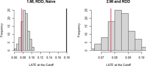
Table 5 displays the results of the analyses, replicating the analyses in Lee (2008). The estimates from MIRDD and RDD are 0.084 and 0.077, respectively, meaning that the estimated incumbency advantage is about 8% of the vote share (Lee 2008, p. 690). The 95% confidence intervals are ${CI}_{95\mathrm{\%}}\left(0.067,\mathrm{ }0.101\right)$ and ${CI}_{95\mathrm{\%}}\left(0.060,\mathrm{ }0.094\right),$ respectively. Thus, we are 95% confident that the incumbency advantage at the cutoff point is roughly 6 to 10% of the vote share.

Table 5. Results of the analyses.

	Estimate	Std. Error	CI.LL	CI.UL	n	Ratio	Bandwidth
MIRDD ($M=100$)	0.084	0.009	0.067	0.101	2761	42.1	0.25
RDD	0.077	0.009	0.060	0.094	2761	42.1	0.25
Naïve	0.179	0.006	0.167	0.191	2761	42.1	0.25

Notes: Estimate is an estimated LATE at the cutoff, Std. Error is the standard error, CI.LL is the lower limit of the 95% confidence interval, CI.UL is the upper limit of the 95% confidence interval, n is the subsample size, ratio is the ratio of the subsample to the original sample size, and bandwidth is the length of bandwidth used in the discontinuity analyses.

Note that, the bandwidth in Table 5 is about twice as large as the automatically selected size by mserd. The simulations reported in Table 1 and in the Online Appendix A showed that a narrower bandwidth tended to lead to better results. Readers can freely use the software in the Appendix to see how different settings may affect the conclusions we make. Below, we will diagnose whether the results in Table 5 are reasonable or not.

Figure 1 graphically presents the results in Table 5. The solid black line is the Naïve estimator, the solid red line is RDD, and the histogram is MIRDD ($M=100$). We can visually confirm that Naïve is far away from MIRDD and RDD, while RDD is within the distribution of MIRDD. When the conclusions from MIRDD and RDD agree, it still may not guarantee that the conclusion is correct, but we may feel more confident, because the disagreement between MIRDD and RDD indicates that at least one of them is wrong.

Figure 1. Graphical presentation of the naïve estimator, RDD, and MIRDD ($M=100$).

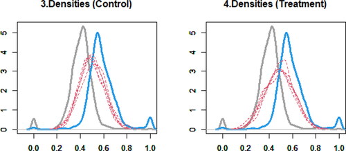
Figure 2 presents the densities of observed and imputed data in the control and treatment groups, where the gray solid curve is the density of observed data in the control group, the blue solid curve is the density of observed data in the treatment group, and the red dashed curves are the densities of imputed data. We look for anomalous shapes in imputed data compared to observed data. These figures show that the distributions of imputed data are consistent with the implications from observed data. Comparing the densities of observed and imputed data is a standard diagnostic technique in multiple imputation of missing data (Abayomi, Gelman, and Levy 2008, p. 277; Honaker, King, and Blackwell 2011, p. 26; van Buuren 2018, p. 193).

Figure 2. Densities of observed and imputed data ($M=5$) in the control and treatment groups.

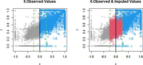
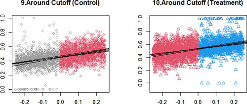
Figure 3 presents the scatterplots of observed and imputed data. The black solid line is the cutoff point. The green dashed lines are the bandwidths, where the RDD analysis is performed. Gray circles are the observed data in the control group, and blue triangles are the observed data in the treatment group. Red circles are the imputed data for the control group, and red triangles are the imputed data for the treatment group. The distributions of imputed data look consistent with those of observed data; however, the distributions of imputed data overlap those of observed data, making it somewhat hard to visualize.

Figure 3. Scatterplots of observed and imputed data ($M=1$).

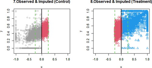
To provide clearer pictures, Figure 4 divides the right-hand side panel in Figure 3 into two figures. In Figure 4, the left-hand panel focuses on the control group, and the right-hand panel focuses on the treatment group. Beyond the cutoff point, red circles and red triangles are the extrapolation, respectively. Based on the implications from the observed data (gray circles and blue triangles), the extrapolation looks reasonable.

Figure 4. Left-hand panel is the scatterplot of observed and imputed data ($M=1$) in the control group, and right-hand panel is the scatterplot of observed and imputed data ($M=1$) in the treatment group.

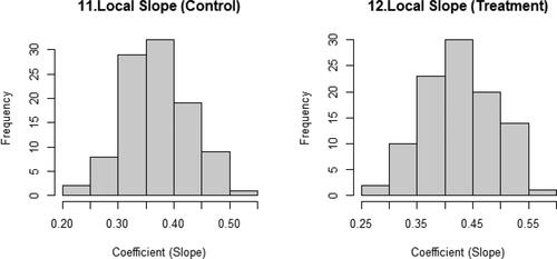
Figure 5 further magnifies Figure 4, focusing on the local area chosen by the bandwidth. In this case, the horizontal axis ranges from −0.25 to 0.25. Five solid lines are the estimated local slopes based on imputed data. These figures confirm that local linearity approximately holds in this example.

Figure 5. Local area chosen by the bandwidth. Imputed data ($M=1$) and estimated slopes ($M=5$).

Figure 6 presents the histograms of the local slopes for the control and treatment groups. Figure 5 showed only five lines, so as to clearly show the scatterplot. Figure 6 displays the distribution of all of the $M$ local slopes. These figures show the estimation uncertainty in the local area, meaning that if the distributions are too wide or oddly shaped, we are less certain of the results.

Figure 6. Histograms of the local slopes for the control and the treatment groups based on imputed data ($M=100$).

6. Conclusion

The RDD is one of the strongest causal inference methods for non-experimental data, because RDDs focus on the small enough neighborhood around the cutoff point, so that subgroups can be treated as de-facto randomly assigned groups. Thus, RDDs can estimate the LATE at the cutoff point. This article found that the proposed method (MIRDDs) can also estimate the LATE at the cutoff point, just as equally well as RDDs. Based on this finding, this article proposed a graphical method based on MIRDDs to diagnose the validity of RDD analyses. This is an important addition to the literature of RDDs in particular and of causal inference in general, because graphical assessments are an integral part of RDD analyses. Furthermore, an easy-to-use software program is provided that implements the methods explained in this article.

Appendix

To implement the approaches introduced in this article, the author has written easy-to-use software, R-package MIRDD. The software and documentation are freely available at https://github.com/mtakahashi123/MIRDD. Essentially, analysis can be easily done by just typing MIdiagRDD(y, x, cut) in R, with a variety of other options also available. Replication materials for the simulations are deposited at https://github.com/mtakahashi123/replication1.