A comparison of normality testing methods by empirical power and distribution of P-values

Abstract

Normal distribution is commonly assumed distribution in statistical inference. Therefore, goodness-of-fit test for normality is required as a preliminary procedure in the applications. Most relevant testing methods have been evaluated using empirical power. However, the power depends on significance level, sample size, and alternative distributions. This study compares normality testing methods which have been verified excellent based on power, considering significance levels, sample sizes, and alternative distributions in addition to their powers. Furthermore we evaluate the performance of the testing methods using the expected and median values of p-values of the corresponding test statistics.

Keywords:

• Goodness-of-fit test
• Normality test
• Power comparison
• P-value

1. Introduction

Normal distribution is the most commonly assumed distribution in statistical inferential procedures and whose feasibility depends on how well the assumed distribution fits to normal distribution. Therefore the goodness-of-fit (GOF) test for normality is a required preliminary procedure before applying relevant statistical applications. There have been numerous goodness-of-fit tests for normality. Most of them are based on empirical power and their results are often inconsistent and dependent upon significance level α. Thus there have been suggestions of considering sample size and significance level α in addition to the power (Sackrowitz and Samuel-Cahn 1999; Yazici and Yolacan 2007; Mbah and Paothong 2015).

Dempster and Schatzoff (1965) introduced the concept of the expected significance level and discussed the stochastic aspect of the p-value. Sackrowitz and Samuel-Cahn (1999) elaborated the approach, proposed the expected p-value (EPV), and presented extensive potential for the utilization of EPV in various aspects of hypothesis tests. The distribution of p-values under the null hypothesis is known to follow U(0,1). However, its distribution under the alternative hypothesis is skewed to the right and Bhattacharya and Habtzghi (2002) proposed the median of the p-value (MPV) as a better measure of performance than EPV.

In this study we select tests of normality which have been verified excellent based on power, and investigate their performances in terms of power as varying sample size, significance level α, and distributional forms under alternative hypotheses. Furthermore the results of their performances are compared with those of EPV and MPV as well.

2. Normality testing methods

In this section we review briefly the nine testing methods which have been verified excellent by the performance measure of power. Table 1 presents the acronyms of each method used in this study in reference to tests of normality.

Table 1. Abbreviations for each normality testing method.

Testing method	Abbreviation
Lilliefors	M.KS
Cramer von Mises	CVM
Anderson-Darling	AD
Zhang-Wu ZC	ZC
Zhang-Wu ZA	ZA
Jarque-Bera	JB
Gel-Gastwirth	R.JB
Shapiro-Wilk	SW
Shapiro-Francia	SF

2.1. Empirical distribution function

Let $X_1,\dots ,X_n$ be a random sample from a population with cumulative distribution function (CDF) $F(·)$ and its order statistics $X_{(1)}\le X_{(2)}\le \cdots \le X_{(n)}.$ The empirical cumulative distribution function (ECDF) $F_n(x)$ is defined in terms of the indicator function $\mathbf{1}(·)$ as follows: $$F_n(x)=\frac{1}{n}\sum _{i=1}^n\mathbf{1}(X_{(i)}\le x).$$

2.1.1. Lilliefors’ revised Kolmogorov-Smirnov test

The Kolmogorov–Smirnov (KS) assumed that two parameters, mean and variance, of normal distribution are known. However it is uncommon to have both parameters known and most cases are with at least one parameter estimated. For such cases, Lilliefors (1967) modified the KS test statistic for the test of normality as follows: $$\mathrm{M}.{\text{KS}}_{\mathit{n}}=\underset{\mathit{x}\in \mathit{R}}{\mathit{sup}}\left|{\mathit{F}}_{\mathit{n}}(\mathit{x})-\Phi \left(\frac{\mathit{x}-\widehat{\mu }}{\widehat{\sigma }}\right)\right|=\mathit{max}(\mathrm{M}.{\text{KS}}_{\mathit{n}}^{+},\mathrm{M}.{\text{KS}}_{\mathit{n}}^{-}),$$ where $\mathrm{M}.{\text{KS}}_{\mathit{n}}^{+}=\underset{\mathit{x}\in \mathit{R}}{\mathit{sup}}{|\mathit{F}}_{\mathit{n}}(\mathit{x})-\Phi ((\mathit{x}-\widehat{\mu })/\widehat{\sigma })|,$ $\mathrm{M}.{\text{KS}}_{\mathit{n}}^{-}=\underset{\mathit{x}\in \mathit{R}}{\mathit{sup}}|\Phi ((\mathit{x}-\widehat{\mu })/\widehat{\sigma }){-\mathit{F}}_{\mathit{n}}(\mathit{x})|,$ $\widehat{\mu }=\overline{X},\widehat{\sigma }=\sqrt{\sum {(X_i-\overline{X})}^2/(n-1)}$ and $\Phi (x)$ is the CDF of the standard normal distribution.

2.1.2. Cramer-von Mises test

The Cramer-von Mises test for a hypothesized distribution F₀ was developed by Cramer, von Mises, and Smirnov and defined by (Cramer 1928; Von Mises 1932; Smirnov 1936; Conover 1999), $$\text{CVM}={\int }_{-\infty }^{\infty }{\left[F_n(x)-F_0(x)\right]}^{2}d{F}_0(x).$$

2.1.3. Anderson-Darling test

Anderson and Darling (1954) related the concept of the weighted mean to the CVM test statistic, assigning more weight to the tail of ${\left[F_n(x)-F_0(x)\right]}^2,$ and proposed the following test statistic $$\text{AD}={\int }_{-\infty }^{\infty }{\left[F_n(x)-F_0(x)\right]}^2\Psi \left(F_0(x)\right)d{F}_0(x),$$ where $\Psi (F_0(x))={\left\{F_0(x)(1-F_0(x))\right\}}^{-1}.$

2.1.4. Zhang-Wu test

Not only is Zhang credited with the creation of the KS, CVM, and AD test statistics, but also proposed new and more powerful types of test statistics, as follows (Zhang 2002; Zhang and Wu 2005): $$\begin{array}{c}\text{ZC}=\sum _{i=1}^n{\left[\text{ln}\hspace{0.17em}\left\{\frac{\left(1/\Phi (z_{(i)})-1\right)}{(n-0.5)/(i-0.75)-1}\right\}\right]}^2,\\ \text{ZA}=-\sum _{i=1}^n\left[\frac{\hspace{0.17em}\text{ln}\hspace{0.17em}\Phi (z_{(i)})}{n-i+0.5}+\frac{\hspace{0.17em}\text{ln}\hspace{0.17em}\left[1-\Phi (z_{(i)})\right]}{i-0.5}\right],\end{array}$$ where $z_{(i)}=(x_{(i)}-\overline{x})/s$ and $s=\sqrt{{\sum }_{i=1}^n{(x_{(i)}-\overline{x})}^2/(n-1)}.$

2.2. Moments

2.2.1. Jarque-Bera test

The Jarque-Bera test was proposed by Bowman and Shenton and elaborated by Jarque and Bera and defined by (Bowman and Shenton 1975; Jarque and Bera 1987; Romao, Delgado, and Costa 2010) as $$\text{JB}=\frac{n}{6}\left(b_1+\frac{{(b_2-3)}^2}{4}\right),$$ where $\sqrt{b_1}=m_3/m_2{}^{3/2}$ and $b_2=m_4/m_2^2$ with $m_r={\sum }_{i=1}^n{(x_i-\overline{x})}^r/n.$

2.2.2. Gel-Gastwirth test

Henderson (2006) pointed out that sample moments are not insensitive to outliers as they provide equal weights to all observations. Gel and Gastwirth (2008) proposed the following robust form of the Gel-Gastwirth (R.JB) test statistic $$\mathrm{R}.\text{JB}=\frac{\mathit{n}}{6}{\left(\frac{{\mathit{m}}_3}{{\mathit{J}}_{\mathit{n}}^3}\right)}^2+\frac{\mathit{n}}{64}{\left(\frac{{\mathit{m}}_4}{{\mathit{J}}_{\mathit{n}}^4}-3\right)}^2,$$ where J_n is an estimate of variance which is less sensitive to outliers, defined by $$J_n=\frac{\sqrt{\pi /2}}{n}\sum _{i=1}^n| x_i-\text{med}(x_1,\dots ,x_n)|.$$

2.3. Regression and correlation

2.3.1. Shapiro-Wilk test

Shapiro and Wilk (1965) proposed the following test statistic, using the mean vector m and covariance matrix V of order statistics of a random sample of size n from standard normal distribution and a vector of ordered random observations $y={(y_1\le \cdots \le y_n)}^{\prime },$ $$\text{SW}=\frac{{\left(\sum _{i=1}^n{a}_i{y}_i\right)}^2}{\sum _{i=1}^n{(y_i-\overline{y})}^2},$$ where $a^{\prime }=(a_1,\dots ,a_n)=\frac{m^{\prime }{V}^{-1}}{{(m^{\prime }{V}^{-1}{V}^{-1}m)}^{1/2}}.$

2.3.2. Shapiro–Francia test

In the statistic SW, the values of m and V are not easy to obtain, and especially the calculation of $V^{-1}$ consumes huge time with large sample size. Shapiro and Francia (1972) overcame it by proposing an identity matrix instead of $V^{-1}$ in the statistic SW, defined as $$\text{SF}=\frac{{(\sum _{i=1}^n{b}_i{y}_i)}^2}{\sum _{i=1}^n{(y_i-\overline{y})}^2},$$ where $(b_1,\dots ,b_n)=\frac{m^{\prime }}{{(m^{\prime }m)}^{1/2}}.$

3. The simulation results

In this section we compare the empirical powers of the nine aforementioned normality testing methods as varying sample size n, significance level α and distributional form under alternative hypothesis. Furthermore the distributional characteristics such as mean and median of the p-values of the test statistics are used to evaluate the performances of the testing methods. We did Monte Carlo simulations with 100,000 repetitions for the cases displayed at Table 2. The similar simulation has been performed by Uhm (2020) for the scenarios with larger samples and empirical type I error.

Table 2. Simulation conditions: alternative distributions, sample sizes and significance levels.

Distribution		Sample size	α
	Beta(2)
Symmetric	Laplace(0,1)
	t(1)
		10,20,30,100,200,300	0.01, 0.05
	Beta(1, 2)
Asymmetric	${\chi }^2$(1)
	Gamma(2)

3.1. Performances by empirical power

Table 3 summarizes the empirical powers of the testing methods by the test statistics listed on the first row for various alternative distributions as sample size n gets increased at significance level $\alpha =0.01.$ When alternative distribution is symmetric Beta(2,2), the testing methods by ZC and ZA show the best power up to the sample size 30 and the sample size of 100 or larger, respectively. The testing methods by ZA, SW and SF have their powers decreased despite of increasing the sample size from 10 to 20, and the ones by JB and R.JB show the same pattern up to the sample size 100. When alternative distribution is Laplace or t-distribution, the testing method by R.JB has the best power among all the methods considered.

Table 3. Empirical power: empirical power for various normality tests depending on sample size n under each alternative distribution at $\alpha =0.01.$

distribution under Ha		n	M.KS	CVM	AD	ZC	ZA	JB	R.JB	SW	SF
symmetric	Beta(2,  2)	10	0.0086	0.0068	0.0065	0.0130	${0.0097}^{*}$	${0.0006}^{*}$	${0.0126}^{*}$	${0.0060}^{*}$	${0.0042}^{*}$
		20	0.0090	0.0085	0.0091	0.0131	${0.0096}^{*}$	${0.0003}^{*}$	${0.0028}^{*}$	${0.0048}^{*}$	${0.0019}^{*}$
		30	0.0109	0.0127	0.0142	0.0200	0.0173	${0.0001}^{*}$	${0.0008}^{*}$	0.0083	0.0019
		100	0.0349	0.0706	0.1025	0.2171	0.3091	${0.0000}^{*}$	${0.0000}^{*}$	0.1318	0.0330
		200	0.1046	0.2571	0.3976	0.7209	0.8913	0.0514	0.0011	0.6540	0.3571
		300	0.2130	0.5014	0.7134	0.9421	0.9961	0.5608	0.1595	0.9528	0.8080
	Laplace(0,  1)	10	0.0504	0.0572	0.0605	0.0867	0.0906	0.0266	0.1587	0.0646	0.0695
		20	0.0892	0.1235	0.1303	0.1638	0.1610	0.1485	0.3113	0.1312	0.1588
		30	0.1271	0.1888	0.1977	0.2263	0.2126	0.2483	0.4259	0.2034	0.2443
		100	0.4605	0.6500	0.6598	0.5660	0.5257	0.6822	0.8409	0.6362	0.6896
		200	0.8179	0.9424	0.9457	0.8440	0.8263	0.9267	0.9804	0.9292	0.9434
		300	0.9564	0.9938	0.9941	0.9538	0.9500	0.9860	0.9979	0.9902	0.9924
	t(1)	10	0.4429	0.4818	0.4832	0.4918	0.5062	0.3439	0.6013	0.4752	0.4905
		20	0.7485	0.8067	0.8093	0.7853	0.7979	0.7633	0.8887	0.7923	0.8178
		30	0.8936	0.9324	0.9342	0.9132	0.9187	0.9159	0.9681	0.9256	0.9384
		100	0.9999	1.0000	1.0000	0.9999	1.0000	1.0000	1.0000	1.0000	1.0000
		200	1.0000	1.0000	1.0000	1.0000	1.0000	1.0000	1.0000	1.0000	1.0000
		300	1.0000	1.0000	1.0000	1.0000	1.0000	1.0000	1.0000	1.0000	1.0000
asymmetric	Beta(2,  1)	10	0.0256	0.0283	0.0306	0.0522	0.0492	0.0042	${0.0419}^{*}$	0.0326	0.0241
		20	0.0532	0.0740	0.0874	0.1183	0.1498	0.0117	${0.0413}^{*}$	0.0836	0.0510
		30	0.0944	0.1490	0.1849	0.2257	0.3433	0.0134	${0.0389}^{*}$	0.1984	0.1095
		100	0.5537	0.7888	0.9049	0.9296	0.9981	0.1669	0.1147	0.9762	0.9161
		200	0.9534	0.9962	0.9999	0.9988	1.0000	0.9806	0.8595	1.0000	1.0000
		300	0.9992	1.0000	1.0000	1.0000	1.0000	1.0000	0.9998	1.0000	1.0000
	${\chi }^2(1)$	10	0.3070	0.4445	0.4723	0.5522	0.5742	0.1754	0.4341	0.5101	0.4577
		20	0.6986	0.8646	0.8987	0.9148	0.9622	0.5841	0.7562	0.9248	0.8920
		30	0.9203	0.9793	0.9894	0.9883	0.9988	0.8289	0.9030	0.9956	0.9898
		100	1.0000	1.0000	1.0000	1.0000	1.0000	1.0000	1.0000	1.0000	1.0000
		200	1.0000	1.0000	1.0000	1.0000	1.0000	1.0000	1.0000	1.0000	1.0000
		300	1.0000	1.0000	1.0000	1.0000	1.0000	1.0000	1.0000	1.0000	1.0000
	Gamma(2,  2)	10	0.0605	0.0774	0.0860	0.1368	0.1413	0.0345	0.1530	0.1013	0.0947
		20	0.1412	0.2186	0.2530	0.3454	0.3913	0.1991	0.3161	0.2986	0.2785
		30	0.2351	0.3689	0.4310	0.5377	0.6365	0.3468	0.4491	0.5184	0.4714
		100	0.8292	0.9589	0.9843	0.9903	0.9997	0.9497	0.9417	0.9972	0.9942
		200	0.9957	1.0000	1.0000	1.0000	1.0000	1.0000	0.9999	1.0000	1.0000
		300	1.0000	1.0000	1.0000	1.0000	1.0000	1.0000	1.0000	1.0000	1.0000

Note: The boldface denotes the best performance for each sample size.

The asterisk$(*)$ shows that the empirical power decreases as the sample size increases up to moderate sample sizes.

When alternative distribution is asymmetric Beta(2,1), the method by R.JB has the power decreased as sample size n increases up to 30, and increased from n = 100, which is the case with Beta(2,2). The power by ZA shows the highest value among all sample cases except for n = 10. When alternative distribution is chi-squared, the method by ZA shows the highest power in all samples. The method by ZA has the highest power in all samples except for n = 10 at the alternative of gamma distribution.

Table 4 summarizes the power of the nine testing methods at the significance level $\alpha =0.05.$ Compared with $\alpha =0.01,$ their powers get increased at $\alpha =0.05,$ which confirms the fact that the power of test gets increased as significance level does. The opposite direction of the power by ZA and SW methods for sample size up to n = 20 shown at $\alpha =0.01$ does not appear at $\alpha =0.05.$ However the methods by JB and SF show the opposite phenomenon up to n = 30 and the ones by R.JB up to n = 100. For the other cases, the method by R.JB is best for the alternative of Laplace and t-distribution, and the one by ZA has the best power for all asymmetric alternative distributions, which are the same as in the case of $\alpha =0.01.$

Table 4. Empirical power: empirical power for various normality tests depending on sample size n under each alternative distribution at $\alpha =0.05.$

distribution under Ha		n	M.KS	CVM	AD	ZC	ZA	JB	R.JB	SW	SF
symmetric	Beta(2,  2)	10	0.0447	0.0435	0.0439	0.0538	0.0386	${0.0027}^{*}$	${0.0215}^{*}$	0.0419	${0.0328}^{*}$
		20	0.0487	0.0549	0.0566	0.0694	0.0433	${0.0011}^{*}$	${0.0064}^{*}$	0.0532	${0.0234}^{*}$
		30	0.0572	0.0713	0.0766	0.1027	0.0684	${0.0005}^{*}$	${0.0022}^{*}$	0.0774	0.0277
		100	0.1527	0.2434	0.3157	0.5802	0.5703	0.0148	${0.0002}^{*}$	0.4522	0.2170
		200	0.3369	0.5516	0.7081	0.9679	0.9783	0.6135	0.2529	0.9232	0.7532
		300	0.5340	0.7921	0.9189	0.9992	0.9998	0.9633	0.7929	0.9970	0.9739
	Laplace(0,  1)	10	0.1409	0.1564	0.1594	0.1620	0.1811	0.0631	0.2069	0.1540	0.1868
		20	0.2172	0.2653	0.2707	0.2582	0.2785	0.2163	0.3821	0.2609	0.3189
		30	0.2894	0.3633	0.3708	0.3348	0.3490	0.3353	0.5087	0.3566	0.4269
		100	0.7066	0.8227	0.8273	0.7049	0.7021	0.7791	0.8984	0.7966	0.8457
		200	0.9444	0.9829	0.9836	0.9271	0.9273	0.9628	0.9907	0.9748	0.9825
		300	0.9920	0.9988	0.9988	0.9859	0.9867	0.9948	0.9993	0.9975	0.9984
	t(1)	10	0.5756	0.6089	0.6098	0.5839	0.6144	0.4249	0.6466	0.5894	0.6317
		20	0.8425	0.8784	0.8804	0.8459	0.8649	0.8162	0.9109	0.8659	0.8927
		30	0.9434	0.9633	0.9643	0.9450	0.9527	0.9407	0.9766	0.9582	0.9686
		100	1.0000	1.0000	1.0000	1.0000	1.0000	1.0000	1.0000	1.0000	1.0000
		200	1.0000	1.0000	1.0000	1.0000	1.0000	1.0000	1.0000	1.0000	1.0000
		300	1.0000	1.0000	1.0000	1.0000	1.0000	1.0000	1.0000	1.0000	1.0000
asymmetric	Beta(2,  1)	10	0.0984	0.1144	0.1238	0.1507	0.1326	0.0144	0.0627	0.1319	0.1111
		20	0.1709	0.2286	0.2614	0.3300	0.3331	0.0306	0.0706	0.3054	0.2162
		30	0.2622	0.3621	0.4260	0.5406	0.5935	0.0429	0.0771	0.5150	0.3720
		100	0.8211	0.9386	0.9820	0.9984	0.9999	0.7439	0.4392	0.9987	0.9922
		200	0.9962	0.9998	1.0000	1.0000	1.0000	0.9999	0.9991	1.0000	1.0000
		300	1.0000	1.0000	1.0000	1.0000	1.0000	1.0000	1.0000	1.0000	1.0000
	${\chi }^2(1)$	10	0.5329	0.6627	0.6951	0.7468	0.7532	0.2722	0.4985	0.7329	0.7051
		20	0.8775	0.9514	0.9688	0.9837	0.9901	0.7162	0.8177	0.9836	0.9732
		30	0.9822	0.9957	0.9983	0.9996	0.9999	0.9199	0.9426	0.9996	0.9991
		100	1.0000	1.0000	1.0000	1.0000	1.0000	1.0000	1.0000	1.0000	1.0000
		200	1.0000	1.0000	1.0000	1.0000	1.0000	1.0000	1.0000	1.0000	1.0000
		300	1.0000	1.0000	1.0000	1.0000	1.0000	1.0000	1.0000	1.0000	1.0000
	Gamma(2,  2)	10	0.1692	0.2047	0.2226	0.2599	0.2656	0.0766	0.1971	0.2407	0.2427
		20	0.3190	0.4193	0.4651	0.5449	0.5742	0.2888	0.3921	0.5313	0.5039
		30	0.4593	0.5981	0.6600	0.7559	0.7974	0.4746	0.5458	0.7492	0.7068
		100	0.9529	0.9912	0.9974	0.9998	1.0000	0.9916	0.9838	0.9998	0.9993
		200	0.9997	1.0000	1.0000	1.0000	1.0000	1.0000	1.0000	1.0000	1.0000
		300	1.0000	1.0000	1.0000	1.0000	1.0000	1.0000	1.0000	1.0000	1.0000

Note: The boldface denotes the best performance for each sample size.

The asterisk$(*)$ shows that the empirical power decreases as the sample size increases up to moderate sample sizes.

3.2. Performances by the distributional characteristics of p-values

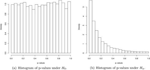
Let F₀ and $F_{\theta }$ denote the cumulative distribution of the test statistics T under H₀ and $T^{\ast }$ under H_a, respectively. Sackrowitz and Samuel-Cahn (1999) defined the EPV under H_a as $E_T\left[P(T^{\ast }\ge T|T)\right]=P(T^{\ast }>T)=\text{EPV}(\theta )$ and showed that the EPV is stochastically smaller under H_a than under H₀, which implies that the smaller EPV means the stronger evidence for H_a. It is also known that under the null hypothesis F₀ follows uniform distribution on (0, 1), and the mean and median of the distribution of p-values are always 0.5. The plots at Figure 1 show the empirical distribution of p-values under $H_0:N(0,1)$ and $H_a:N(1,1),$ respectively. The distribution of p-values under H_a is skewed to the right, in which case the median is a better measure of the central tendency of the distribution than the mean. It motivates the use of the MPV, not the EPV, as a performance measure of the normality testing methods. The testing method with the smaller MPV is a better one, for the smaller p-value tells more clearly the difference between the null and alternative.

Figure 1. The empirical distributions of p-values under $H_0:N(0,1)$ and $H_a:N(1,1).$

Tables 5 and 6 are summaries of the EPV and MPV of testing methods, respectively. For the alternative of Beta(2.2), the Table 5 shows that the testing method by ZC yields the smallest EPV up to n = 100 and the one by ZA does for n greater than or equal to 200. For the alternative of Laplace distribution, the testing method by AD and SF has the smallest mean p-value up to n = 30, while the method by SF does for alternative of t-distribution. When we have the alternative of asymmetric Beta(2,1), the method by ZC has the smallest expected p-value up to the sample size 20, and the one by ZA does for the sample size greater than 20. For the alternative distribution of chi-square and gamma, the method by ZC has the smallest EPV for n = 10 and the one by ZA does for the sample size greater than 10.

Table 5. Expected P-values: The expected value of the distribution of p-values for various normality tests depending on each sample size under each alternative distribution.

distribution under Ha		n	M.KS	CVM	AD	ZC	ZA	JB	R.JB	SW	SF
symmetric	Beta(2,  2)	10	0.5004	0.4792	0.4683	0.4618	0.5041	0.6863	0.7181	0.4748	0.5201
		20	0.4855	0.4586	0.4478	0.3977	0.4757	0.6063	0.6695	0.4287	0.5059
		30	0.4588	0.4265	0.4090	0.3203	0.4040	0.5347	0.6139	0.3695	0.4745
		100	0.2977	0.2369	0.1868	0.0769	0.0947	0.2095	0.2992	0.1104	0.2058
		200	0.1613	0.0964	0.0546	0.0137	0.0077	0.0539	0.1033	0.0158	0.0425
		300	0.0894	0.0389	0.0156	0.0035	0.0005	0.0138	0.0355	0.0022	0.0078
	Laplace(0,  1)	10	0.3992	0.3799	0.3748	0.4302	0.3869	0.5906	0.5111	0.4146	0.3815
		20	0.3261	0.2986	0.2953	0.3418	0.2821	0.4401	0.3443	0.3334	0.2771
		30	0.2662	0.2341	0.2300	0.3026	0.2481	0.3424	0.2457	0.2620	0.2077
		100	0.0688	0.0429	0.0421	0.1022	0.0826	0.0737	0.0319	0.0541	0.0380
		200	0.0116	0.0039	0.0038	0.0160	0.0134	0.0092	0.0022	0.0057	0.0040
		300	0.0022	0.0004	0.0003	0.0036	0.0034	0.0012	0.0001	0.0006	0.0004
	t(1)	10	0.1619	0.1478	0.1466	0.1997	0.1603	0.2964	0.2000	0.1710	0.1455
		20	0.0487	0.0386	0.0378	0.0541	0.0397	0.0779	0.0407	0.0466	0.0340
		30	0.0147	0.0099	0.0096	0.0242	0.0155	0.0217	0.0090	0.0125	0.0085
		100	0.0000	0.0000	0.0000	0.0000	0.0000	0.0000	0.0000	0.0000	0.0000
		200	0.0000	0.0000	0.0000	0.0000	0.0000	0.0000	0.0000	0.0000	0.0000
		300	0.0000	0.0000	0.0000	0.0000	0.0000	0.0000	0.0000	0.0000	0.0000
asymmetric	Beta(2,  1)	10	0.4103	0.3743	0.3533	0.3237	0.3592	0.6051	0.6286	0.3414	0.3854
		20	0.3182	0.2665	0.2348	0.1736	0.1946	0.4362	0.4861	0.1915	0.2481
		30	0.2408	0.1838	0.1476	0.1005	0.0986	0.3199	0.3778	0.1026	0.1521
		100	0.0325	0.0122	0.0044	0.0040	0.0002	0.0381	0.0647	0.0013	0.0036
		200	0.0019	0.0003	0.0000	0.0004	0.0000	0.0018	0.0052	0.0000	0.0000
		300	0.0001	0.0000	0.0000	0.0001	0.0000	0.0001	0.0004	0.0000	0.0000
	${\chi }^2(1)$	10	0.1279	0.0873	0.0738	0.0602	0.0631	0.2836	0.2393	0.0621	0.0736
		20	0.0244	0.0100	0.0065	0.0047	0.0024	0.0585	0.0504	0.0040	0.0061
		30	0.0041	0.0011	0.0005	0.0008	0.0001	0.0124	0.0111	0.0003	0.0006
		100	0.0000	0.0000	0.0000	0.0000	0.0000	0.0000	0.0000	0.0000	0.0000
		200	0.0000	0.0000	0.0000	0.0000	0.0000	0.0000	0.0000	0.0000	0.0000
		300	0.0000	0.0000	0.0000	0.0000	0.0000	0.0000	0.0000	0.0000	0.0000
	Gamma(2,  2)	10	0.3513	0.3175	0.2991	0.2892	0.2977	0.5114	0.4934	0.2932	0.3117
		20	0.2315	0.1843	0.1598	0.1243	0.1238	0.2664	0.2674	0.1302	0.1487
		30	0.1534	0.1070	0.0840	0.0622	0.0548	0.1432	0.1497	0.0567	0.0705
		100	0.0096	0.0022	0.0008	0.0008	0.0000	0.0021	0.0028	0.0002	0.0003
		200	0.0000	0.0000	0.0000	0.0000	0.0000	0.0000	0.0000	0.0000	0.0000
		300	0.0000	0.0000	0.0000	0.0000	0.0000	0.0000	0.0000	0.0000	0.0000

Note: The boldface denotes the best performance for each sample size.

Table 6. Median P-values: The median value of the distribution of p-values for various normality tests depending on each sample size under each alternative distribution.

distribution under Ha		n	M.KS	CVM	AD	ZC	ZA	JB	R.JB	SW	SF
symmetric	Beta(2,  2)	10	0.5015	0.4682	0.4620	0.4474	0.4909	0.6903	0.7537	0.4582	0.5182
		20	0.4789	0.4363	0.4298	0.3405	0.4276	0.5965	0.6710	0.3902	0.5020
		30	0.4420	0.3903	0.3734	0.2155	0.3120	0.5167	0.6018	0.3168	0.4604
		100	0.2345	0.1600	0.1120	0.0369	0.0336	0.1812	0.2675	0.0596	0.1417
		200	0.0948	0.0392	0.0175	0.0073	0.0006	0.0395	0.0810	0.0050	0.0180
		300	0.0435	0.0099	0.0028	0.0027	0.0000	0.0086	0.0243	0.0005	0.0024
	Laplace(0,  1)	10	0.3527	0.3263	0.3275	0.4290	0.3800	0.6596	0.6383	0.3792	0.3141
		20	0.2398	0.2009	0.1964	0.2268	0.1772	0.4562	0.2190	0.2369	0.1597
		30	0.1642	0.1176	0.1134	0.1866	0.1136	0.2456	0.0432	0.1355	0.0818
		100	0.0133	0.0026	0.0022	0.0115	0.0135	0.0001	0.0000	0.0025	0.0017
		200	0.0006	0.0000	0.0000	0.0007	0.0004	0.0000	0.0000	0.0000	0.0000
		300	0.0000	0.0000	0.0000	0.0001	0.0001	0.0000	0.0000	0.0000	0.0000
	t(1)	10	0.0210	0.0128	0.0127	0.0151	0.0148	0.1390	0.0000	0.0148	0.0112
		20	0.0001	0.0000	0.0000	0.0000	0.0000	0.0000	0.0000	0.0000	0.0000
		30	0.0000	0.0000	0.0000	0.0000	0.0000	0.0000	0.0000	0.0000	0.0000
		100	0.0000	0.0000	0.0000	0.0000	0.0000	0.0000	0.0000	0.0000	0.0000
		200	0.0000	0.0000	0.0000	0.0000	0.0000	0.0000	0.0000	0.0000	0.0000
		300	0.0000	0.0000	0.0000	0.0000	0.0000	0.0000	0.0000	0.0000	0.0000
asymmetric	Beta(2,  1)	10	0.3751	0.3235	0.3022	0.2314	0.2664	0.6274	0.7059	0.2795	0.3289
		20	0.2487	0.1856	0.1515	0.1024	0.1174	0.4430	0.5334	0.1132	0.1694
		30	0.1585	0.0983	0.0714	0.0530	0.0457	0.3135	0.4026	0.0470	0.0843
		100	0.0072	0.0012	0.0003	0.0029	0.0000	0.0288	0.0569	0.0002	0.0008
		200	0.0001	0.0000	0.0000	0.0004	0.0000	0.0010	0.0035	0.0000	0.0000
		300	0.0000	0.0000	0.0000	0.0000	0.0000	0.0000	0.0002	0.0000	0.0000
	${\chi }^2(1)$	10	0.0408	0.0154	0.0124	0.0175	0.0138	0.2621	0.0515	0.0092	0.0131
		20	0.0021	0.0002	0.0001	0.0005	0.0000	0.0024	0.0000	0.0002	0.0004
		30	0.0001	0.0000	0.0000	0.0002	0.0000	0.0000	0.0000	0.0000	0.0000
		100	0.0000	0.0000	0.0000	0.0000	0.0000	0.0000	0.0000	0.0000	0.0000
		200	0.0000	0.0000	0.0000	0.0000	0.0000	0.0000	0.0000	0.0000	0.0000
		300	0.0000	0.0000	0.0000	0.0000	0.0000	0.0000	0.0000	0.0000	0.0000
	Gamma(2,  2)	10	0.2854	0.2404	0.2203	0.2315	0.2414	0.5750	0.6350	0.2064	0.2147
		20	0.1340	0.0809	0.0618	0.0453	0.0370	0.2389	0.1746	0.0415	0.0489
		30	0.0624	0.0263	0.0170	0.0121	0.0050	0.0626	0.0255	0.0087	0.0122
		100	0.0005	0.0000	0.0000	0.0002	0.0000	0.0000	0.0000	0.0000	0.0000
		200	0.0000	0.0000	0.0000	0.0000	0.0000	0.0000	0.0000	0.0000	0.0000
		300	0.0000	0.0000	0.0000	0.0000	0.0000	0.0000	0.0000	0.0000	0.0000

Note: The boldface denotes the best performance for each sample size.

Table 6 shows the result of MPV for each testing method. When the alternative distribution is symmetric Beta(2,2), the testing methods by ZC up to n = 30 and by ZA for n greater than or equal to 100 produce the smallest median p-value, respectively. For the alternative of Laplace distribution, the methods by SF up to the sample size 20 and by R.JB for the sample size greater than or equal to 30 have the smallest median p-value, respectively. The method by R.JB yields the smallest MPV for the alternative of t distribution. When we have asymmetric Beta(2,1) for the alternative, the performance of the testing methods is the same as that of the symmetric Beta(2,2). When we have the alternative distribution of chi-square and gamma, however, we found the method by SW for n = 10 and by ZA for n greater than 10 the best, respectively.

For the alternative of Beta(2,2) the powers of the testing method by JB and R.JB get decreased while the sample size increases up to 100. However, the EPV and MPV of those two methods decrease monotonically as the sample size increases. The phenomenon that the representative values such as EPV or MPV decrease monotonically as the sample sizes gets increased is observed at all the testing methods under the study. The JB method performs well by the MPV, but does not by the EPV. All the methods by the test statistics except for AD and SF show the same performance as well.

Figures 2–6 display the pattern of the EPV and MPV according as the sample size changes. All the testing methods by the test statistics except for JB and R.JB show that the lines of the EPV and MPV don’t cross over across the sample size and the line of the MPV converges to zero faster than that of the EPV.

Figure 2. The distributional features of p-values when using Lilliefors’ modified Kolmogorov-Smirnov test statistic with varying sample size under the asymmetric alternative distributions. The dotted line and solid line are the expected value and the median value of the p-values, respectively.

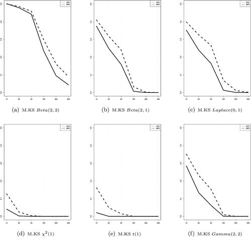
Figure 3. The distributional features of p-values when using Cramer von-Mises and Anderson-Darling test statistics with varying sample size under the asymmetric alternative distributions. The dotted line and solid line are the expected value and the median value of the p-values, respectively.

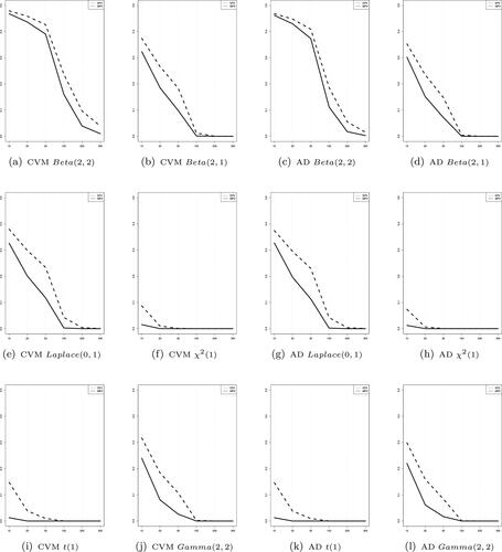
Figure 4. The distributional features of p-values when using Zhang-Wu test statistics with varying sample size under the asymmetric alternative distributions. The dotted line and solid line are the expected value and the median value of the p-values, respectively.

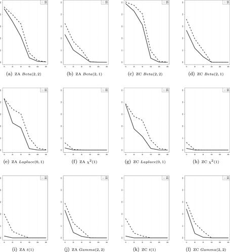
Figure 5. The distributional features of p-values when using Jarque-Bera and Gel-Gastwirth (R.JB) test statistics with varying sample size under the asymmetric alternative distributions. The dotted line and solid line are the expected value and the median value of the p-values, respectively.

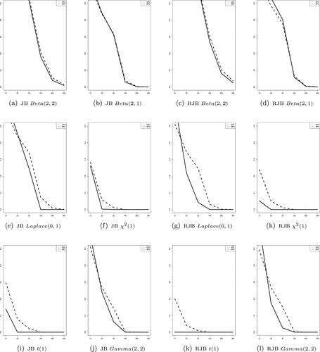
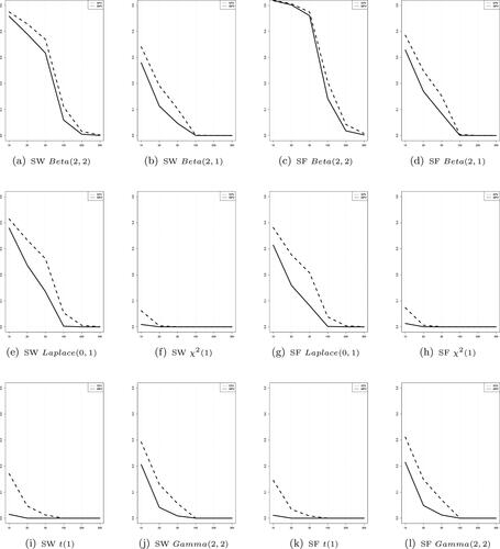
Figure 6. The distributional features of p-values when using Shapiro-Wilk and Shapiro-Francia test statistics with varying sample size under the asymmetric alternative distributions. The dotted line and solid line are the expected value and the median value of the p-values, respectively.

4. Conclusion

In this study we have compared the performances of the widely accepted normality testing methods in terms of testing power and the distributional features of p-values under various conditions of alternative distributions, sample sizes and significance levels. The powers of the testing methods don’t show consistency over the significance level and they get decreased as the sample size increases.

On the contrary the representative values such as the EPV or MPV show consistency, or decrease monotonically as the sample size gets increased. The performances by the EPV are similar to those by the MVP as a whole, but there are some testing methods showing opposite performances. The convergence of the MPV to zero is faster than that of the EPV.

As a recap, we suggest the following guideline in selection of normality testing methods:

• ZC when data is of small size $(n\le 30)$ and shows symmetric distribution.

• ZA when data is of moderate size $(30<n\le 300)$ and shows symmetric distribution.

• ZC when data is of small size $(n\le 30)$ and shows asymmetric distribution.

• ZA when data is of moderate size $(30<n\le 300)$ and shows asymmetric distribution.

Considering the above results, as a performance criterion for normality testing method, the MPV is preferred to the EPV in that the distribution of p-values is skewed. The MPV is also preferred to the power of the tests, for the latter does not show insensitivity to the choice of the significance level.

Acknowledgements

This work was supported by the Pukyong National University Research Fund in 2020.

References

- Anderson, T. W., and D. A. Darling. 1954. A test of goodness of fit. Journal of the American Statistical Association 49 (268):765–209. doi:10.1080/01621459.1954.10501232.
- Bhattacharya, B., and D. Habtzghi. 2002. Median of the p-value under the alternative hypothesis. The American Statistician 56 (3):202–206. doi:10.1198/000313002146.
- Bowman, K. O., and L. R. Shenton. 1975. Omnibus test contours for departures from normality based on b1 and b2. Biometrika 62 (2):243–50.
- Conover, W. J. 1999. Practical nonparametric statistics. New York: Wiley.
- Cramer, H. 1928. On the composition of elementary errors: first paper: mathematical deductions. Scandinavian Actuarial Journal 1928 (1):13–74.
- Dempster, A. P., and M. Schatzoff. 1965. Expected significance level as a sensitivity index for test statistics. Journal of the American Statistical Association 60 (310):420–36. doi:10.1080/01621459.1965.10480802.
- Gel, Y. R., and J. L. Gastwirth. 2008. A robust modification of the Jarque-Bera test of normality. Economics Letters 99 (1):30–32. doi:10.1016/j.econlet.2007.05.022.
- Henderson, A. R. 2006. Testing experimental data for univariate normality. Clinica Chimica Acta; International Journal of Clinical Chemistry 366 (1-2):112–29. doi:10.1016/j.cca.2005.11.007.
- Jarque, C. M., and A. K. Bera. 1987. A test for normality of observations and regression residuals. International Statistical Review / Revue Internationale de Statistique 55 (2):163–72. doi:10.2307/1403192.
- Lilliefors, H. W. 1967. On the Kolmogorov-Smirnov test for normality with mean and variance unknown. Journal of the American Statistical Association 62 (318):399–402. doi:10.1080/01621459.1967.10482916.
- Mbah, A. K., and A. Paothong. 2015. Shapiro-Francia test compared to other normality test using expected p-value. Journal of Statistical Computation and Simulation 85 (15):3002–16. doi:10.1080/00949655.2014.947986.
- Romao, X., R. Delgado, and A. Costa. 2010. An empirical power comparison of univariate goodness-of-fit tests for normality. Journal of Statistical Computation and Simulation 80 (5):545–91. doi:10.1080/00949650902740824.
- Sackrowitz, H., and E. Samuel-Cahn. 1999. P values as random variables expected P values. The American Statistician 53 (4):326–31. doi:10.2307/2686051.
- Shapiro, S. S., and R. S. Francia. 1972. An approximate analysis of variance test for normality. Journal of the American Statistical Association 67 (337):215–16. doi:10.1080/01621459.1972.10481232.
- Shapiro, S. S., and M. B. Wilk. 1965. An analysis of variance test for normality. Biometrika 52 (3-4):591–611. doi:10.1093/biomet/52.3-4.591.
- Smirnov, N. V. 1936. Sui la distribution de w2. Comptes Rendus 202:449–52.
- Uhm, T. W. 2020. Comparison of the normality tests using the distribution of p-values. unpublished Ph.D. diss., Pukyong National University, Dept. of Statistics, Korea.
- Von Mises, R. 1932. Wahrscheinlichkeitsrechnung und ihre Anwendung in der Statistik und theoretischen Physik. Bulletin of the American Mathematical Society 38:169–70.
- Yazici, B., and S. Yolacan. 2007. A comparison of various tests of normality. Journal of Statistical Computation and Simulation 77 (2):175–83. doi:10.1080/10629360600678310.
- Zhang, J. 2002. Powerful goodness-of-fit tests based on the likelihood ratio. Journal of the Royal Statistical Society: Series B (Statistical Methodology) 64 (2):281–94. doi:10.1111/1467-9868.00337.
- Zhang, J., and Y. Wu. 2005. Likelihood-ratio tests for normality. Computational Statistics & Data Analysis 49 (3):709–21. doi:10.1016/j.csda.2004.05.034.