The generalized sigmoidal quantile function

Abstract

In this note we introduce a new smooth nonparametric quantile function estimator based on a newly defined generalized expectile function and termed the sigmoidal quantile function estimator. We also introduce a hybrid quantile function estimator, which combines the optimal properties of the classic kernel quantile function estimator with our new generalized sigmoidal quantile function estimator. The generalized sigmoidal quantile function can estimate quantiles beyond the range of the data, which is important for certain applications given smaller sample sizes. This property of extrapolation is illustrated in order to improve standard bootstrap smoothing resampling methods.

Keywords:

• Bootstrap
• Expectiles
• Hermitian quantile function
• Kernel quantile estimator
• Tail extrapolation

1. Introduction

It is well known that a continuous random variable X can be described not only in terms of its p.d.f. $f(·),$ and its c.d.f. $F(·),$ but also in terms of the lesser known quantile function $Q(·).$ For a general distribution function, which is continuous from the right the conventional definition of the quantile function is given by (1.1) $$Q(u)=\inf \{x:F(x)>u\}.$$(1.1)

Furthermore, if $F(·)$ is absolutely continuous then $Q(u)=F^{-1}(u)$ has a unique value. This allows one to also define the density-quantile function as $f(Q(u))=1/Q\prime (u),$ since $F(Q(u))=u$ under the assumption that F is absolutely continuous.

The estimators $\widehat{Q}(u)$ of the population quantiles, $0<u<1,$ are of interest in a broad spectrum of theories, methods and applications of parametric, robust and exploratory statistical analyses. Their importance is emphasized in the following quote from Parzen (1993) where he wishes to “….emphasize to applied statisticians our opinion that the first step in data analysis should be to form the sample quantile function, $Q^{(n)}(u),0<u<1,$….”

While the population quantile function may be unique there are a variety of estimators each with their respective strengths and weakness. As background let $X_{1:n}<X_{2:n}<\cdots <X_{n:n}$ denote the order statistic from an i.i.d. sample of size n from a continuous distribution F with support over the entire real line. Some well-known quantile function estimators take the following forms: (1.2) $${\widehat{Q}}_S(u)=X_{[nu]+1:n}$$(1.2) (1.3) $${\widehat{Q}}_L(u)=(1-ϵ)X_{[n\prime u]:n}+ϵX_{[n\prime u]+1:n},$$(1.3) (1.4) $${\widehat{Q}}_H(u)=w_1{X}_{[n\prime u-1/2]:n}+w_2{X}_{[n\prime u-1/2]+1:n}+w_3{X}_{[n\prime u-1/2]+2:n},$$(1.4) (1.5) $${\widehat{Q}}_K(u)={\displaystyle {\int }_0^1{h}^{-1}}k\left(\frac{t-u}{h}\right){\widehat{Q}}_S(t)dt,$$(1.5) (1.6) $${\widehat{Q}}_{HD}(u)=\sum _{j=1}^n{w}_{j(u)}{X}_{j:n},$$(1.6) where $0<u<1,[·]$ denotes the floor function, $n\prime =n+1$ and the subscripts correspond to S=simple, L=linear interpolation, H=Hermitian (Mudholkar, Hutson, and Marchetti (2001)), K=Kernel (e.g., see Sheather and Marron (1990)), HD=Harrell-Davis (Harrell and Davis (1982). Other nonparametric estimators include special L-estimators termed generalized order statistics and Bernstein polynomial type estimators as discussed in Cheng (1995). The specific weighting functions for (1.4)-(1.6) are given as follows:

1. For the ${\widehat{Q}}_L(u)$ estimator the weights are given as (1.7) $$ϵ=n\prime u-[n\prime u].$$(1.7)

2. For the ${\widehat{Q}}_H(u)$ estimator the weights are given as (1.8) $$w_1=\frac{1}{2}-\tau +\frac{{\tau }^2}{2},w_2=\frac{1}{2}+\tau -{\tau }^2,w_3=1-w_1-w_2,$$(1.8) (1.9) $$\text{and \hspace{0.17em}\hspace{0.17em}}\tau =(n\prime u-1/2-[n\prime u-1/2]).$$(1.9)

3. For the ${\widehat{Q}}_K(u)$ estimator the weights are defined with $k(·)$ being a p.d.f. on R (symmetric about 0) with h serving as the bandwidth parameter, where h > 0. For h = 0, i.e. $k(·)$ is generate, ${\widehat{Q}}_K(u)$ reduces to ${\widehat{Q}}_S(u)$ type form. The empirical version of the weighting function general takes the form $w_j=F((\frac{j}{n}-u)/h)-F((\frac{j-1}{n}-u)/h),$ where $F(·)$ denotes a given cumulative distribution function from a location-scale family of distributions.

4. For the ${\widehat{Q}}_{HD}(u)$ estimator the weights are given as (1.10) $$w_{j(u)}=B_{(n+1)u,(n+1)(1-u)}\left(\frac{j}{n}\right)-B_{(n+1)u,(n+1)(1-u)}\left(\frac{j-1}{n}\right)$$(1.10)

and $B_{p,q}(x)$ is the cumulative distribution function for a beta function with shape parameters p, q

Kernel quantile estimators have been extensively studied and analyzed for efficiency and bias tradeoffs, e.g., see Sheather and Marron (1990), Reiss (1980, 1989) and the references therein. However, few of the more efficient kernel estimators are used in common practice. The most commonly employed estimator, in applications such as Q-Q plots and incorporated in popular software packages such as SAS, R, and MINITAB, is the linear interpolation between two neighboring order statistics. However, ${\widehat{Q}}_L(u)$ lacks smoothness and does not provide a useful density quantile function estimate. It is interesting to note that ${\widehat{Q}}_{HD}(u)$ at (1.6)(1.6) $${\widehat{Q}}_{HD}(u)=\sum _{j=1}^n{w}_{j(u)}{X}_{j:n},$$(1.6) can be interpreted as the estimator of the expectation of an order statistic, where order is defined on a continuous scale and termed a fractional order statistic by Stigler (1977). Similarly, the utilization of the simple quantile function ${\widehat{Q}}_S(u)$ at (1.3)(1.3) $${\widehat{Q}}_L(u)=(1-ϵ)X_{[n\prime u]:n}+ϵX_{[n\prime u]+1:n},$$(1.3) can be used to derive so-called exact bootstrap calculations about a statistical functional T(F), e.g., see Hutson and Ernst (2000) for an example involving L-estimators.

If we let $U\sim (U(0,1)$ then generating a univariate bootstrap sample with replacement may be viewed as simulating data from ${\widehat{Q}}_S(u),$ i.e., one bootstrap replicate is given by $X^{*}={\widehat{Q}}_S(U).$ Hence, one approach to smoothing a bootstrap resample, particularly in the small sample setting, is to utilize $X^{*}={\widehat{Q}}_K(U).$ The choice between quantile estimators is often a tradeoff between bias (rates of convergence), variance and smoothness relative to the application at hand, which is one motivation of our new proposed estimator. See Hutson (2000, 2002) for various quantile based resampling approaches. Alternative kernel smoothing approaches include introducing a smoothing function, i.e., add some noise to the resample value for a given kernel bandwidth, e.g., see Polansky and Schucany (1997). We argue that smoothing is less important in fact than extrapolation given small sample sizes. Quantile-based bootstrap extrapolation methods will be an area of investigation in this note.

An alternative formulation of the population uth quantile for the random variable X is given by the value of θ satisfying (1.11) $$\underset{\theta \in \mathcal{R}}{\inf }E\left\{\frac{|X-\theta |+(2u-1)(X-\theta )}{2}-\frac{\left|X\right|+(2u-1)X}{2}\right\}.$$(1.11)

The properties of the expression at (1.11)(1.11) $$\underset{\theta \in \mathcal{R}}{\inf }E\left\{\frac{|X-\theta |+(2u-1)(X-\theta )}{2}-\frac{\left|X\right|+(2u-1)X}{2}\right\}.$$(1.11) are outlined in Abdous and Theodorescu (1992) who generalize the definition of the α-quantile to ${\mathcal{R}}^k$ space, $k\ge 1.$ Most notably, the assumption that $E(X)<\infty ,\alpha \in (0,1),$ in (1.11)(1.11) $$\underset{\theta \in \mathcal{R}}{\inf }E\left\{\frac{|X-\theta |+(2u-1)(X-\theta )}{2}-\frac{\left|X\right|+(2u-1)X}{2}\right\}.$$(1.11) is not a necessary condition for the existence of the uth quantile. Given $F(·)$ is absolutely continuous (1.11)(1.11) $$\underset{\theta \in \mathcal{R}}{\inf }E\left\{\frac{|X-\theta |+(2u-1)(X-\theta )}{2}-\frac{\left|X\right|+(2u-1)X}{2}\right\}.$$(1.11) can be reduced to (1.12) $$\underset{\theta \in \mathcal{R}}{\inf }E\left\{|X-\theta |+(2u-1)(X-\theta )\right\}.$$(1.12)

A natural extension to the regression setting is to replace θ in (1.12)(1.12) $$\underset{\theta \in \mathcal{R}}{\inf }E\left\{|X-\theta |+(2u-1)(X-\theta )\right\}.$$(1.12) with a continuous function $g(·)$ of a set of p covariates $\mathbf{x}=(x_1,x_2,\dots ,x_p)$ (oftentimes setting $x_1=1$ when an intercept term is involved) and p regression parameters $\mathit{\beta }\prime =({\beta }_0,{\beta }_1,\dots ,{\beta }_{p-1}).$ This substitution defines the population conditional quantile function as an expectation and minimization problem of the form (1.13) $$Q_{\mathit{\beta }}(u|\mathbf{x})=\underset{\mathit{\beta }\in {\mathcal{R}}^p}{\inf }E\left\{|Y-g(\mathit{x}\prime \mathit{\beta })|+(2u-1)(Y-g(\mathit{x}\prime \mathit{\beta }))\right\}.$$(1.13)

For example, if $g(\mathit{x}\prime \mathit{\beta })={\beta }_0+{\beta }_{1}x$ and $\alpha =1/2,$ then equation (1.13)(1.13) $$Q_{\mathit{\beta }}(u|\mathbf{x})=\underset{\mathit{\beta }\in {\mathcal{R}}^p}{\inf }E\left\{|Y-g(\mathit{x}\prime \mathit{\beta })|+(2u-1)(Y-g(\mathit{x}\prime \mathit{\beta }))\right\}.$$(1.13) would correspond to assuming a model for which the conditional median of Y given x is linear in x, i.e., least absolute deviations (LAD) regression or L₁ regression, e.g., see Hutson (2018). Similar well-known formulations exist that all lend themselves well to the regression setting, e.g., see the classic paper of Bassett and Koenker (1982). Note that none of the estimators at (1.3)(1.3) $${\widehat{Q}}_L(u)=(1-ϵ)X_{[n\prime u]:n}+ϵX_{[n\prime u]+1:n},$$(1.3) -(1.6)(1.6) $${\widehat{Q}}_{HD}(u)=\sum _{j=1}^n{w}_{j(u)}{X}_{j:n},$$(1.6) readily translates to the quantile regression setting.

The limitations of quantile regression are well-known and center on issues related to the discreteness of the L₁ norm and non-uniqueness of solutions. This partially motivated the rise of expectiles where the L₁ norm in (1.12)(1.12) $$\underset{\theta \in \mathcal{R}}{\inf }E\left\{|X-\theta |+(2u-1)(X-\theta )\right\}.$$(1.12) may be replaced by the L₂ norm. We use a slightly modified definition of an expectile with very similar properties to the original definition such that for our purposes we define the uth expectile as the value of θ such that (1.14) $$\underset{\theta \in \mathcal{R}}{\inf }E\left\{{(X-\theta )}^2+(2u-1)(X-\theta )\right\},$$(1.14) assuming $E(X^2)<\infty ,$ e.g., see Abdous and Remillard (1995), Jones (1994), Koenecker (1993) and more recently Mao, Ng, and Hu (2015) for a set of excellent theoretical treatments of the subject. Newey and Powell (1987) developed the framework for asymmetric least-squares regression methods.

In this note we examine how the well-known sigmoid approach to approximating the absolute value function, which not only provides an alternative quantile smoothing function approach based on (1.12)(1.12) $$\underset{\theta \in \mathcal{R}}{\inf }E\left\{|X-\theta |+(2u-1)(X-\theta )\right\}.$$(1.12) but also interestingly provides a direct link to approximating the expectile function at (1.14)(1.14) $$\underset{\theta \in \mathcal{R}}{\inf }E\left\{{(X-\theta )}^2+(2u-1)(X-\theta )\right\},$$(1.14) . Applications include smooth quantile estimation and smooth bootstrap resampling procedures, which readily generalize to the regression setting.

In Sec. 1 we provide background into quantile function estimation and introduce several of the well-known quantile function estimators. In Sec. 2 we provide some preliminaries around the sigmoidal function approximation to the absolute value function. In Sec. 3 we implement the sigmoidal function estimator to define a new class of generalized expectiles, which can be used to define a smooth quantile function estimator termed the generalized sigmoidal quantile function estimator. In Sec. 4 we introduce the theoretical properties of this estimator, which is a specific case of an M-estimator. We also intoduce a new hybrid quantile function estimator, which combines the optimal properties of the classic kernel quantile function estimator with the generalized sigmoidal quantile function estimator. In Sec. 5 we compare the various quantile function estimators across light to heavy-tailed distributions in terms of bias and variance tradeoffs across interior and extreme quantiles. In Sec. 6 we illustrate how the two new quantile function estimators provide more accurate bootstrap percentile intervals due to the addition of tail extrapolated based information. In Sec. 7 we provide a real data example comparing the various quantile function estimators. Finally, in Sec. 8 we provide some concluding remarks.

2. Sigmoid function preliminaries

A convenient form of sigmoid function for our application relative to approximating the absolute value function is given through the logistic cumulative distribution function with mean 0 and variance τ and given as: (2.1) $$F(y)=\frac{1}{1+e^{-\frac{y}{\tau }}},$$(2.1) where $\tau >0.$ First define the plus function as ${(x)}_{+}={\int }_{-\infty }^x\sigma (y)dy,$ where $\sigma (x)$ is the step function (2.2) $$\sigma (x)=\{\begin{array}{cc}1\hfill & \text{if\hspace{0.17em}}x>0\hfill \\ 0\hfill & \text{if\hspace{0.17em}}x\le 0.\hfill \end{array}$$(2.2)

Chen and Mangasarian (1995) illustrate that we can approximate the plus function as follows: (2.3) $${(x)}_{+}\approx {\int }_{-\infty }^{x}F(y)dy=\tau \hspace{0.17em}\text{log}\hspace{0.17em}\left(e^{\frac{x}{\tau }}+1\right),$$(2.3) where F is defined at (2.1). Using the result at (2.3) Schmidt, Fung, and Rosales (2007) derive the approximation for the absolute value function given (slightly reparametrized for our purposes) as (2.4) $$\left|x\right|={(x)}_{+}+{(-x)}_{+}\approx g_{\tau }(x)=\tau \left(\hspace{0.17em}\text{log}\hspace{0.17em}\left(e^{\frac{x}{\tau }}+1\right)+\hspace{0.17em}\text{log}\hspace{0.17em}\left(e^{-\frac{x}{\tau }}+1\right)\right),$$(2.4) as $\tau \to 0.$ Note that in the computational optimization world the approximation at (2.4) is often parameterized in terms of $\alpha =1/\tau .$ However, we chose the form (2.4) in order to better to align with bandwidth smoothing procedures used in statistical practice.

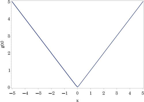
Framing the absolute value approximation in statistical terms allows one to note that the c.d.f. at (2.1)(2.1) $$F(y)=\frac{1}{1+e^{-\frac{y}{\tau }}},$$(2.1) corresponds to a degenerate distribution as $\tau \to 0$ such that it is clearly a step-function at x = 0 in the limit. See Figure 1 for a plot of the approximation at the value $\tau =0.1.$ The interest in the sigmoid-based approximation to the absolute value function stems from the fact that higher order derivatives of $g{(x)}_{\tau }$ with respect to x exist at x = 0. Hence, this provides the ability to derive gradient and Hessian functions for stable numerical optimization routines, which in turn allows for unique numerical solutions, whereas the estimator based on the function (1.14)(1.14) $$\underset{\theta \in \mathcal{R}}{\inf }E\left\{{(X-\theta )}^2+(2u-1)(X-\theta )\right\},$$(1.14) may not have a unique solution for a given value for u due to discreteness issues.

Figure 1. Plot of $g{(x)}_{0.1}.$

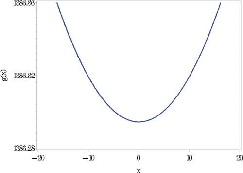
Interestingly and to the best of our knowledge examination of the behavior of $g{(x)}_{\tau }$ at (2.4)(2.4) $$\left|x\right|={(x)}_{+}+{(-x)}_{+}\approx g_{\tau }(x)=\tau \left(\hspace{0.17em}\text{log}\hspace{0.17em}\left(e^{\frac{x}{\tau }}+1\right)+\hspace{0.17em}\text{log}\hspace{0.17em}\left(e^{-\frac{x}{\tau }}+1\right)\right),$$(2.4) as $\tau \to \infty$ has not been examined in the computational optimization world for obvious reasons. From a statistical point of view one can view that the logistic distribution will behave similarly to a Bayesian non-informative prior over the real-line such that as $\tau \in {\mathbb{R}}^{+}$ then as $\tau \to \infty ,$ F(y) converges to a uniform (Lebesgue) distribution. It follows straightforward that as $\tau \to \infty$ that $g{(x)}_{\tau }$ approximates a quadratic function of the form $(x^2+a)/c$ similar to when as $\tau \to 0$ that $g{(x)}_{\tau }$ approximates an absolute value function. See Figure 2 for an example at τ = 1000. The ramifications of this simple observation will be of interest in terms of a link between quantiles and expectiles as described in the next section.

Figure 2. Plot of $g{(x)}_{1000}.$

3. The generalized sigmoidal quantile function: Definition, estimation and properties

The generalized sigmoidal quantile function (GSQF) is based on a modification of (1.12)(1.12) $$\underset{\theta \in \mathcal{R}}{\inf }E\left\{|X-\theta |+(2u-1)(X-\theta )\right\}.$$(1.12) of the quantile function defined as (3.1) $$Q(u)=\underset{\theta \in \mathcal{R}}{\inf }E\left\{|X-\theta |+(2u-1)(X-\theta )\right\}$$(3.1) and described earlier. This is accomplished by substituting the absolute value function $|·|$ at (3.1) with its smooth counterpart, $g{(x)}_{\tau }$ defined at (2.4), to arrive at the form of the GSQF given as: (3.2) $$Q_{\tau }(u)=\underset{{\theta }_{\tau }\in \mathcal{R}}{\inf }E\left\{g_{\tau }(X-{\theta }_{\tau })+(2u-1)(X-{\theta }_{\tau })\right\},$$(3.2) (3.3) $$=\underset{{\theta }_{\tau }\in \mathcal{R}}{\inf }E\left\{\tau \left(\hspace{0.17em}\text{log}\hspace{0.17em}\left(e^{-\frac{X-{\theta }_{\tau }}{\tau }}+1\right)+\hspace{0.17em}\text{log}\hspace{0.17em}\left(e^{\frac{X-{\theta }_{\tau }}{\tau }}+1\right)\right)+(2u-1)(X-{\theta }_{\tau })\right\}.$$(3.3)

It should be immediately obvious that in the limit $Q_{\tau }(u)\to Q(u)$ as $\tau \to 0,$ i.e.,

$E\left\{g_{\tau }(X-{\theta }_{\tau })+(2u-1)(X-{\theta }_{\tau })\right\}\to E\left\{|X-{\theta }_{\tau }|+(2u-1)(X-{\theta }_{\tau })\right\}$ as $\tau \to 0.$ The function $Q_{\tau }(u)$ at (3.3)(3.3) $$=\underset{{\theta }_{\tau }\in \mathcal{R}}{\inf }E\left\{\tau \left(\hspace{0.17em}\text{log}\hspace{0.17em}\left(e^{-\frac{X-{\theta }_{\tau }}{\tau }}+1\right)+\hspace{0.17em}\text{log}\hspace{0.17em}\left(e^{\frac{X-{\theta }_{\tau }}{\tau }}+1\right)\right)+(2u-1)(X-{\theta }_{\tau })\right\}.$$(3.3) falls within a class of functions termed “smoothed Huber estimators”, as described in Hampel, Hennig, and Ronchetti (2011), albeit the GSQF having a slightly different form of objective function. The smooth Huber estimators rely on a normal c.d.f. to define the smoothing component whereas we employ the logistic c.d.f. as described above to arrive at $g{(x)}_{\tau },$ which in turn provides more mathematically tractable results for our application.

For a fixed u and τ the sample GSQF estimator for (3.3)(3.3) $$=\underset{{\theta }_{\tau }\in \mathcal{R}}{\inf }E\left\{\tau \left(\hspace{0.17em}\text{log}\hspace{0.17em}\left(e^{-\frac{X-{\theta }_{\tau }}{\tau }}+1\right)+\hspace{0.17em}\text{log}\hspace{0.17em}\left(e^{\frac{X-{\theta }_{\tau }}{\tau }}+1\right)\right)+(2u-1)(X-{\theta }_{\tau })\right\}.$$(3.3) then becomes (3.4) $$\begin{array}{c}{\widehat{Q}}_{\tau }(u)=\underset{{\widehat{\theta }}_{\tau }\in \mathcal{R}}{\inf }\frac{1}{n}\sum _{i=1}^n\left\{\tau \left(\hspace{0.17em}\text{log}\hspace{0.17em}\left(e^{-\frac{X_i-{\widehat{\theta }}_{\tau }}{\tau }}+1\right)+\hspace{0.17em}\text{log}\hspace{0.17em}\left(e^{\frac{X_i-{\widehat{\theta }}_{\tau }}{\tau }}+1\right)\right)+(2u-1)(X_i-{\widehat{\theta }}_{\tau })\right\},\\ =\underset{{\widehat{\theta }}_{\tau }\in \mathcal{R}}{\inf }{h}_{\tau }(\mathbf{X};{\widehat{\theta }}_{\tau }),\end{array}$$(3.4) which is similar to the step function estimator ${\widehat{Q}}_S(u)$ at (1.3) as $\tau \to 0$ and becomes more “smooth” for $\tau \gg 0.$

In terms of finding the numerical solution for (3.4)(3.4) $$\begin{array}{c}{\widehat{Q}}_{\tau }(u)=\underset{{\widehat{\theta }}_{\tau }\in \mathcal{R}}{\inf }\frac{1}{n}\sum _{i=1}^n\left\{\tau \left(\hspace{0.17em}\text{log}\hspace{0.17em}\left(e^{-\frac{X_i-{\widehat{\theta }}_{\tau }}{\tau }}+1\right)+\hspace{0.17em}\text{log}\hspace{0.17em}\left(e^{\frac{X_i-{\widehat{\theta }}_{\tau }}{\tau }}+1\right)\right)+(2u-1)(X_i-{\widehat{\theta }}_{\tau })\right\},\\ =\underset{{\widehat{\theta }}_{\tau }\in \mathcal{R}}{\inf }{h}_{\tau }(\mathbf{X};{\widehat{\theta }}_{\tau }),\end{array}$$(3.4) and arriving at some inferential properties we have that the gradient inherent to the minimization is given by (3.5) $$\frac{d{h}_{\tau }(\mathbf{X},{\widehat{\theta }}_{\tau })}{d{\widehat{\theta }}_{\tau }}=h{\prime }_{\tau }=\frac{1}{n}\sum _{i=1}^n\left(\frac{e^{\frac{{\widehat{\theta }}_{\tau }}{\tau }}-e^{\frac{X_i}{\tau }}}{e^{\frac{{\widehat{\theta }}_{\tau }}{\tau }}+e^{\frac{X_i}{{\tau }_{\tau }}}}-(2u-1)\right),$$(3.5) (3.6) $$=\frac{2}{n}\sum _{i=1}^n\left(\frac{1}{e^{\frac{X_i-{\widehat{\theta }}_{\tau }}{\tau }}+1}-u\right)$$(3.6)

The gradient at (3.6)(3.6) $$=\frac{2}{n}\sum _{i=1}^n\left(\frac{1}{e^{\frac{X_i-{\widehat{\theta }}_{\tau }}{\tau }}+1}-u\right)$$(3.6) has the form such that the estimator ${\widehat{Q}}_{\tau }(u)={\widehat{\theta }}_{\tau }$ falls into the class of classic M-estimators where the solution for ${\widehat{\theta }}_{\tau }$ is may be obtained by numerically solving the following equation: (3.7) $$\frac{d{h}_{\tau }(\mathbf{X},{\widehat{\theta }}_{\tau })}{d{\widehat{\theta }}_{\tau }}=\sum _{i=1}^n\Psi (X_i,{\widehat{\theta }}_{\tau })=0,$$(3.7) where from (3.6) we have $\Psi (X_i,{\widehat{\theta }}_{\tau })=2\left(\frac{1}{e^{\frac{X_i-\widehat{\theta }}{\tau }}+1}-u\right).$ It follows from classic theory that the corresponding M-functional is then given as $E(\Psi (X_i,{\widehat{\theta }}_{\tau }))=\int \Psi (X_i,{\widehat{\theta }}_{\tau })dF(x)=0.$

Under smooth conditions, as outlined in Serfling (1980) and for which our estimator satisfies, we have from classic M-estimator theory that (3.8) $${\widehat{Q}}_{\tau }(u)\sim AN({\theta }_{\tau },n^{-1}{\sigma }^2({\theta }_{\tau }))$$(3.8) for all fixed $\tau >0,$ where ${\sigma }^2({\theta }_{\tau })=\frac{E[\Psi {(X_i,{\theta }_{\tau })}^2]}{E{[\Psi \prime (X_i,{\theta }_{\tau })]}^2}$ given the condition $\Psi \prime (X_i,{\theta }_{\tau })>0,$ where $\Psi \prime (X_i,{\theta }_{\tau })$ is defined below at (3.10). In this setting ${\widehat{Q}}_{\tau }(u)$ could also be considered a generalized expectile function.

In addition, it should be noted that the Hessian is given by (3.9) $$\frac{d^2{h}_{\tau }(\mathbf{X},{\widehat{\theta }}_{\tau })}{d{\widehat{\theta }}_{\tau }^2}=h\prime {\prime }_{\tau }=\frac{1}{n}\sum _{i=1}^n\Psi \prime (X_i,{\widehat{\theta }}_{\tau })=\frac{1}{n}\sum _{i=1}^n\frac{2e^{\frac{{\widehat{\theta }}_{\tau }+X_i}{\tau }}}{\tau {\left(e^{\frac{{\widehat{\theta }}_{\tau }}{\tau }}+e^{\frac{X_i}{\tau }}\right)}^2},$$(3.9) (3.10) $$=\frac{1}{n}\sum _{i=1}^n{\left(\tau \cosh \left(\frac{{\widehat{\theta }}_{\tau }-X_i}{\tau }\right)+\tau \right)}^{-1},$$(3.10) which in turn can be employed as a component for calculating the sandwich variance estimator for ${\widehat{Q}}_{\tau }(u)$ by noting ${\sigma }^2({\theta }_{\tau })$ may be calculated by replacing the population quantities with the sample counterparts for $E[\Psi {(X_i,{\theta }_{\tau })}^2]$ and $E{[\Psi \prime (X_i,{\theta }_{\tau })]}^2,$ respectively.

With respect to the properties of the GSQF estimator we present the following results:

Lemma 1.

For a fixed value of $\tau ,\tau >0,$ and conditional on the observed data $X,$ the function $h_{\tau }(X,{\widehat{\theta }}_{\tau })$ at (3.4) is strictly convex and continuous in ${\widehat{\theta }}_{\tau }.$

Proof.

Follows from equation (3.10)(3.10) $$=\frac{1}{n}\sum _{i=1}^n{\left(\tau \cosh \left(\frac{{\widehat{\theta }}_{\tau }-X_i}{\tau }\right)+\tau \right)}^{-1},$$(3.10) given $\tau >0$ and $\cosh (t)>1$ such that $h_{\tau }^{″}>0,\forall {\widehat{\theta }}_{\tau }\in \mathcal{R}.$

Theorem 1.

For a fixed value of $\tau ,\tau >0,$ and conditional on the observed data $\mathbf{X},$ there is a unique solution to $\underset{{\widehat{\theta }}_{\tau }\in \mathcal{R}}{\inf }{h}_{\tau }(\mathbf{X},{\widehat{\theta }}_{\tau })$ at (3.4).

Proof.

Follows straightforward from Lemma 1, which yields that $h_{\tau }(\mathbf{X},{\widehat{\theta }}_{\tau })$ has a unique global minimum.

Theorem 2.

For a fixed value of $\tau ,\tau >0,$ and conditional on the observed data $\mathbf{X},$ the estimator ${\widehat{Q}}_{\tau }(u)$ at (3.4) is a strictly monotone increasing function as a function of $u:(0,1)\to \mathcal{R}.$

Proof.

For a given u the estimator ${\widehat{Q}}_{\tau }(u)$ is obtained by solving for ${\widehat{\theta }}_{\tau }$ in (3.7), which may be written as solving: (3.11) $$\sum _{i=1}^n\frac{1}{e^{\frac{X_i-{\widehat{\theta }}_{\tau }}{\tau }}+1}=u.$$(3.11)

Noting that ${\sum }_{i=1}^n\frac{1}{e^{\frac{X_i-{\widehat{\theta }}_{\tau }}{\tau }}+1}$ is a strictly monotone increasing function in ${\widehat{\theta }}_{\tau }$ combined with Theorem 1 completes the proof.

Comment. The u-th expectile can be considered for fixed n by letting $\tau \to \infty ,$ i.e., heuristically the expectile is similar to an over-smoothed quantile function relative to choosing a large bandwidth for ${\widehat{Q}}_K(u)={\int }_0^1{h}^{-1}k\left(\frac{t-u}{h}\right)Q_S(t)dt$ at (1.6)(1.6) $${\widehat{Q}}_{HD}(u)=\sum _{j=1}^n{w}_{j(u)}{X}_{j:n},$$(1.6) . As noted in Koenecker (1993) expectiles are in fact quantiles for a given distribution. This observation generalizes that the GSQF is actually a quantile function for all τ, which in turn can be linked back to a given c.d.f. distinct from the c.d.f. from which the underlying sample was generated from.

4. Quantile smoothing and extrapolation

The primary purpose of the GSQF estimator we are advancing is for it to serve as an an alternative to the well-known kernel quantile estimator ${\widehat{Q}}_K(u)$ defined at (1.6)(1.6) $${\widehat{Q}}_{HD}(u)=\sum _{j=1}^n{w}_{j(u)}{X}_{j:n},$$(1.6) or to combine it with ${\widehat{Q}}_K(u)$ to create a hybrid estimator that combines the best features of each distinct quantile function estimator. We argue that the GSQF estimator has better behavior in the tail estimation for Q(u) for densities having support over the whole real line while maintaining the same desirable smoothing properties of those found with the kernel quantile estimator ${\widehat{Q}}_K(u)$ within the range of the data. The same or similar smoothing strategies can be employed for determining a data based choice for the bandwidth τ for ${\widehat{Q}}_{\tau }(u)$ as are used to determine the bandwidth h for ${\widehat{Q}}_K(u)$ in terms of bias and variance tradeoffs.

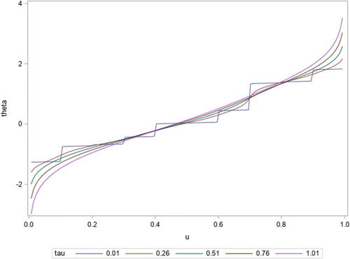
For an introductory illustration of the potential of the GSQF estimator relative to serving as a smooth quantile function estimator we simulated n = 10 observations from a N(0, 1) distribution and calculated ${\widehat{Q}}_{\tau }(u)$ from (3.4)(3.4) $$\begin{array}{c}{\widehat{Q}}_{\tau }(u)=\underset{{\widehat{\theta }}_{\tau }\in \mathcal{R}}{\inf }\frac{1}{n}\sum _{i=1}^n\left\{\tau \left(\hspace{0.17em}\text{log}\hspace{0.17em}\left(e^{-\frac{X_i-{\widehat{\theta }}_{\tau }}{\tau }}+1\right)+\hspace{0.17em}\text{log}\hspace{0.17em}\left(e^{\frac{X_i-{\widehat{\theta }}_{\tau }}{\tau }}+1\right)\right)+(2u-1)(X_i-{\widehat{\theta }}_{\tau })\right\},\\ =\underset{{\widehat{\theta }}_{\tau }\in \mathcal{R}}{\inf }{h}_{\tau }(\mathbf{X};{\widehat{\theta }}_{\tau }),\end{array}$$(3.4) . As one can see from Figure 3 that as τ approaches 0 we approach the step function estimator of the quantile function, ${\widehat{Q}}_S(u).$ However, for very small values of τ we readily start to smooth the quantile function without dramatically modifying the point estimates at a give value of u. So, the theoretical challenge then becomes providing a guideline for the choice of τ if the goal is to use the GSQF as a smooth estimator for the population quantile Q(u). It should be noted that for all of the classic estimators from ${\widehat{Q}}_S(u)$ to ${\widehat{Q}}_{HD}(u)$ at (1.3)(1.3) $${\widehat{Q}}_L(u)=(1-ϵ)X_{[n\prime u]:n}+ϵX_{[n\prime u]+1:n},$$(1.3) - (1.6)(1.6) $${\widehat{Q}}_{HD}(u)=\sum _{j=1}^n{w}_{j(u)}{X}_{j:n},$$(1.6) the function estimates are restricted to the range $[X_{1:n},X_{n:n}]$ regardless of the underlying distribution. The estimator ${\widehat{Q}}_K(u)$ is also limited to the same range to that of ${\widehat{Q}}_S(u),$ whereas the estimator ${\widehat{Q}}_{\tau }(u)$ has the feature of extrapolation in the tail regions, which has important applicability to issues such as extreme value estimation, e.g., estimating a 50 year flood values to smooth bootstrap resampling yielding more precise percentile confidence intervals, e.g., see Hutson (2002).

Figure 3. Example GSQF estimator for $X\sim N(0,1)$ for n = 10 simulated values for various values of τ.

Due to the form of $\Psi (X_i,{\widehat{\theta }}_{\tau })$ at (3.7)(3.7) $$\frac{d{h}_{\tau }(\mathbf{X},{\widehat{\theta }}_{\tau })}{d{\widehat{\theta }}_{\tau }}=\sum _{i=1}^n\Psi (X_i,{\widehat{\theta }}_{\tau })=0,$$(3.7) an analytical expression for the choice of the bandwidth τ in terms of minimizing the mean squared error (MSE) for a given underlying distribution is not readily available. Numerical methods may be applied to solving this problem but are not particularly generalizable. However, data driven choices for the choice of the bandwidth τ may be generated by first noting that from (3.8)(3.8) $${\widehat{Q}}_{\tau }(u)\sim AN({\theta }_{\tau },n^{-1}{\sigma }^2({\theta }_{\tau }))$$(3.8) we may re-express the asymptotic distribution of ${\widehat{Q}}_{\tau }(u)$ from some fixed $u\in (0,1)$ as (4.1) $${\widehat{Q}}_{\tau }(u)\sim AN(Q(u)+\tau b_{\tau }(u),n^{-1}{\sigma }^2({\theta }_{\tau })),$$(4.1) where $\tau b_{\tau }(u)$ denotes the bias of the estimator ${\widehat{Q}}_{\tau }(u)$ relative to estimating Q(u) versus being an asymptotically unbiased estimator of $Q_{\tau }(u)$ given from M-estimation theory.

We can empirically estimate the MSE of ${\widehat{Q}}_{\tau }(u)$ for estimating the quantile function Q(u) at a fixed u by first noting that (4.2) $$\begin{array}{c}MS{E}_{\tau }(u)={(Q_{\tau }(u)-Q(u))}^2+n^{-1}{\sigma }^2({\theta }_{\tau }),\\ ={(Q_{\tau }(u)-Q(u))}^2+n^{-1}\frac{E\left[\Psi {(X_i,{\theta }_{\tau })}^2\right]}{E{[\Psi \prime (X_i,{\theta }_{\tau })]}^2},\\ ={(\tau b_{\tau }(u))}^2+n^{-1}\frac{E\left[\Psi {(X_i,{\theta }_{\tau })}^2\right]}{E{[\Psi \prime (X_i,{\theta }_{\tau })]}^2},\end{array}$$(4.2) and replacing the population quantities with their empirical counterparts, where as before $\Psi (X_i,{\theta }_{\tau })=\frac{e^{\frac{{\theta }_{\tau }}{\tau }}-e^{\frac{X_i}{\tau }}}{e^{\frac{{\theta }_{\tau }}{\tau }}+e^{\frac{X_i}{\tau }}}-(2u-1)$ and $\Psi \prime (X_i,{\theta }_{\tau })=\frac{2e^{\frac{{\theta }_{\tau }+X_i}{\tau }}}{\tau {\left(e^{\frac{{\theta }_{\tau }}{\tau }}+e^{\frac{X_i}{\tau }}\right)}^2}.$ This yields the estimator (4.3) $${\widehat{\mathit{MSE}}}_{\tau }(u)={({\widehat{Q}}_{\tau }(u)-{\widehat{Q}}_K(u))}^2+\frac{\sum _{i=1}^n\Psi {(X_i,{\widehat{Q}}_{\tau }(u))}^2}{{[\sum _{i=1}^n\Psi \prime (X_i,{\widehat{Q}}_{\tau }(u))]}^2},$$(4.3) where ${\widehat{Q}}_K(u)$ is defined at (1.6). Now it should be noted that for fixed u we can simultaneously minimize ${\widehat{\mathit{MSE}}}_{\tau }(u)$ at (4.3) and the function for obtaining ${\widehat{Q}}_{\tau }(u)$ at (3.4) with respect to τ and ${\theta }_{\tau }$ as a dual minimization problem using standard nonlinear programming methods.

Alternatively, a fixed choice for the bandwidth of $\tau =\sigma /\sqrt{n}$ works well in practice and is numerically stable. It should be clear that as $n\to \infty$ for $\tau =\sigma /\sqrt{n}$ that $E\left\{g_{\tau }(X-{\theta }_{\tau })+(2u-1)(X-{\theta }_{\tau })\right\}\to E\left\{|X-{\theta }_{\tau }|+(2u-1)(X-{\theta }_{\tau })\right\}.$ We can utilize $\widehat{\tau }=s/\sqrt{n}$ for unknown σ, where s denotes the sample standard deviation.

Comment. The function $\Psi \prime (X_i,{\theta }_{\tau })$ is numerically unstable for very small values of $\tau \approx 0.05$ or smaller. Care needs to be taken when evaluating this function numerically at these extreme small values due to numerical artifacts. Empirically the jackknife variance estimator and the estimator for the variance of ${\widehat{Q}}_{\tau }(u)$ given by $\frac{{\sum }_{i=1}^n\Psi {(X_i,{\widehat{Q}}_{\tau }(u))}^2}{{[{\sum }_{i=1}^n\Psi \prime (X_i,{\widehat{Q}}_{\tau }(u))]}^2}$ provide virtually identical values for larger values of $\tau >0.1,$ however the jackknife variance estimate is also stable for small values of $\tau <0.1.$

Comment. If the random variable X has a distribution with known support over the positive real line we suggest using the transformation $Y=\hspace{0.17em}\text{log}\hspace{0.17em}(X)$ and then back-transforming to the original scale after estimating Q(u) via the GSQF estimator.

Similar to the approaches found in Hutson (2000, 2002) we wish to also consider the hybrid estimator that combines ${\widehat{Q}}_K(u)$ and ${\widehat{Q}}_{\tau }(u)$ and defined as (4.4) $${\widehat{Q}}_{HB(u)}=\{\begin{array}{ccc}{\widehat{Q}}_{\tau }(u)-{\widehat{Q}}_{\tau }(1/(n+1))+{\widehat{Q}}_K(1/(n+1)),\hfill & \hfill & 0<u\le \frac{1}{n+1},\hfill \\ {\widehat{Q}}_K(u),\hfill & \hfill & \frac{1}{n+1}<u<\frac{n}{n+1},\hfill \\ {\widehat{Q}}_{\tau }(u)-{\widehat{Q}}_{\tau }(n/(n+1))+{\widehat{Q}}_K(n/(n+1)),\hfill & \hfill & \frac{n}{n+1}\le u<1,\hfill \end{array}$$(4.4) where we set $h=u(1-u)/n$ and $\tau =\sigma /\sqrt{n}.$

5. Simulation study

In this section we performed a simulation study to compare the various quantile estimators at (1.3)(1.3) $${\widehat{Q}}_L(u)=(1-ϵ)X_{[n\prime u]:n}+ϵX_{[n\prime u]+1:n},$$(1.3) -(1.6)(1.6) $${\widehat{Q}}_{HD}(u)=\sum _{j=1}^n{w}_{j(u)}{X}_{j:n},$$(1.6) versus the GSQF estimator in terms of bias and variance tradeoffs for quantiles of $u=0.5,0.75,0.9,0.99,0.999$ across the Lapace, Normal and Logistic distributions for sample sizes of n = 10, 25, 50. These three distributions constitute range from light-tailed to heavy tailed distributions. We utilized 10,000 Monte Carlo replications per scenario. We utilized the bandwidth $h=u(1-u)/n$ for the kernel quantile estimator ${\widehat{Q}}_K(u)$ defined at (1.6)(1.6) $${\widehat{Q}}_{HD}(u)=\sum _{j=1}^n{w}_{j(u)}{X}_{j:n},$$(1.6) as per Sheather and Marron (1990). We set $\widehat{\tau }=s/\sqrt{n}$ for the GSQF estimator. The same bandwidths were used for the hybrid estimator ${\widehat{Q}}_{HB}$ defined at (4.4)(4.4) $${\widehat{Q}}_{HB(u)}=\{\begin{array}{ccc}{\widehat{Q}}_{\tau }(u)-{\widehat{Q}}_{\tau }(1/(n+1))+{\widehat{Q}}_K(1/(n+1)),\hfill & \hfill & 0<u\le \frac{1}{n+1},\hfill \\ {\widehat{Q}}_K(u),\hfill & \hfill & \frac{1}{n+1}<u<\frac{n}{n+1},\hfill \\ {\widehat{Q}}_{\tau }(u)-{\widehat{Q}}_{\tau }(n/(n+1))+{\widehat{Q}}_K(n/(n+1)),\hfill & \hfill & \frac{n}{n+1}\le u<1,\hfill \end{array}$$(4.4) . We only provide simulation results for ${\widehat{Q}}_{HB}$ at the extreme quantiles since in the interior the estimator is equivalent to ${\widehat{Q}}_K(u).$

In general we see from Tables 1–3 that ${\widehat{Q}}_{HB}$ appears to be the optimal estimator across all three distributions in terms of bias/variance tradeoffs. Also note that ${\widehat{Q}}_{HB}$ is equivalent to ${\widehat{Q}}_K(u)$ for $1/(n+1)<u<n/(n+1).$ Hence the hybrid estimator benefits through the splicing of ${\widehat{Q}}_{\widehat{\tau }}$ and ${\widehat{Q}}_K(u)$ at both $1/(n+1)$ and $n/(n+1).$ We will examine these set of estimators in the next section relative to bootstrap smoothing applicability.

Table 1. Monte Carlo bias and standard deviation (SD) estimates across competing quantile estimators for $X\sim \mathit{Laplace}(0,1).$

		n = 10		n = 25		n = 50
u	Estimator	bias	SD	bias	SD	bias	SD
0.50	${\widehat{Q}}_{\widehat{\tau }}$	−0.01	0.39	0.00	0.22	0.01	0.16
	${\widehat{Q}}_S$	0.12	0.41	0.00	0.23	0.03	0.16
	${\widehat{Q}}_L$	−0.01	0.39	0.00	0.23	0.01	0.16
	${\widehat{Q}}_H$	−0.01	0.39	0.00	0.22	0.01	0.16
	${\widehat{Q}}_{HD}$	−0.01	0.39	0.00	0.21	0.01	0.15
	${\widehat{Q}}_K$	−0.01	0.39	0.00	0.22	0.01	0.16
0.75	${\widehat{Q}}_{\widehat{\tau }}$	0.24	0.51	0.13	0.32	0.08	0.23
	${\widehat{Q}}_S$	0.04	0.55	−0.01	0.34	0.02	0.25
	${\widehat{Q}}_L$	0.16	0.56	0.07	0.35	0.04	0.25
	${\widehat{Q}}_H$	0.17	0.56	0.07	0.35	0.04	0.25
	${\widehat{Q}}_{HD}$	0.18	0.52	0.09	0.33	0.05	0.24
	${\widehat{Q}}_K$	0.07	0.52	0.04	0.33	0.03	0.24
0.90	${\widehat{Q}}_{\widehat{\tau }}$	0.33	0.91	0.13	0.53	0.06	0.39
	${\widehat{Q}}_S$	0.64	1.31	0.01	0.58	0.11	0.45
	${\widehat{Q}}_L$	0.54	1.22	0.20	0.61	0.09	0.44
	${\widehat{Q}}_H$	0.64	1.31	0.20	0.61	0.09	0.43
	${\widehat{Q}}_{HD}$	0.16	0.95	0.18	0.56	0.09	0.40
	${\widehat{Q}}_K$	0.13	0.91	0.03	0.57	0.01	0.41
0.99	${\widehat{Q}}_{\widehat{\tau }}$	−0.57	1.48	−0.41	1.24	−0.03	1.23
	${\widehat{Q}}_S$	−1.66	1.27	−0.80	1.25	−0.09	1.26
	${\widehat{Q}}_L$	−1.66	1.27	−0.80	1.25	−0.09	1.26
	${\widehat{Q}}_H$	−1.66	1.27	−0.80	1.25	−0.09	1.26
	${\widehat{Q}}_{HD}$	−1.69	1.25	−0.87	1.19	−0.28	1.14
	${\widehat{Q}}_K$	−1.66	1.27	−0.80	1.25	−0.09	1.36
	${\widehat{Q}}_{HB}$	−0.38	1.77	−0.31	1.35	−0.07	1.16
0.999	${\widehat{Q}}_{\widehat{\tau }}$	−1.91	1.74	−2.04	1.37	−1.79	1.31
	${\widehat{Q}}_S$	−3.99	1.24	−3.12	1.25	−2.24	1.27
	${\widehat{Q}}_L$	−3.99	1.24	−3.12	1.25	−2.24	1.27
	${\widehat{Q}}_H$	−3.99	1.24	−3.12	1.25	−2.24	1.27
	${\widehat{Q}}_{HD}$	−3.99	1.24	−3.12	1.25	−2.24	1.26
	${\widehat{Q}}_K$	−3.99	1.24	−3.12	1.25	−2.24	1.27
	${\widehat{Q}}_{HB}$	−1.72	2.01	−1.73	1.65	−1.45	1.53

Table 2. Monte Carlo bias and standard deviation (SD) estimates across competing quantile estimators for $X\sim N(0,1).$

		n = 10		n = 25		n = 50
u	Estimator	bias	SD	bias	SD	bias	SD
0.50	${\widehat{Q}}_{\widehat{\tau }}$	−0.01	0.34	0.01	0.21	0.00	0.16
	${\widehat{Q}}_S$	0.12	0.39	0.01	0.24	0.02	0.17
	${\widehat{Q}}_L$	−0.01	0.37	0.01	0.24	0.00	0.17
	${\widehat{Q}}_H$	−0.01	0.37	0.01	0.23	0.00	0.17
	${\widehat{Q}}_{HD}$	−0.01	0.34	0.01	0.21	0.00	0.16
	${\widehat{Q}}_K$	0-.01	0.36	0.00	0.22	0.01	0.17
0.75	${\widehat{Q}}_{\widehat{\tau }}$	0.08	0.39	0.04	0.25	0.02	0.17
	${\widehat{Q}}_S$	−0.01	0.42	−0.03	0.28	−0.01	0.19
	${\widehat{Q}}_L$	0.07	0.41	0.03	0.27	0.01	0.19
	${\widehat{Q}}_H$	0.07	0.41	0.03	0.27	0.01	0.19
	${\widehat{Q}}_{HD}$	0.05	0.38	0.02	0.25	0.01	0.18
	${\widehat{Q}}_K$	0.00	0.40	0.00	0.26	0.00	0.18
0.90	${\widehat{Q}}_{\widehat{\tau }}$	0.13	0.48	0.08	0.30	0.03	0.21
	${\widehat{Q}}_S$	0.27	0.60	0.00	0.33	0.05	0.24
	${\widehat{Q}}_L$	0.21	0.57	0.11	0.34	0.04	0.24
	${\widehat{Q}}_H$	0.27	0.60	0.11	0.34	0.03	0.24
	${\widehat{Q}}_{HD}$	−0.01	0.48	0.08	0.31	0.03	0.22
	${\widehat{Q}}_K$	−0.01	0.48	0.03	0.32	0.00	0.23
0.99	${\widehat{Q}}_{\widehat{\tau }}$	0.02	0.69	−0.04	0.50	0.00	0.43
	${\widehat{Q}}_S$	−0.79	0.59	−0.36	0.52	−0.08	0.42
	${\widehat{Q}}_L$	−0.79	0.59	−0.36	0.52	−0.08	0.46
	${\widehat{Q}}_H$	−0.79	0.59	−0.36	0.52	−0.08	0.46
	${\widehat{Q}}_{HD}$	−0.81	0.58	−0.39	0.50	−0.15	0.42
	${\widehat{Q}}_K$	−0.79	0.59	−0.36	0.52	−0.08	0.46
	${\widehat{Q}}_{HB}$	0.09	0.80	−0.03	0.57	−0.02	0.45
0.999	${\widehat{Q}}_{\widehat{\tau }}$	−0.01	0.84	−0.33	0.55	−0.39	0.46
	${\widehat{Q}}_S$	−1.55	0.59	−1.13	0.51	−0.84	0.46
	${\widehat{Q}}_L$	−1.55	0.59	−1.13	0.51	−0.84	0.46
	${\widehat{Q}}_H$	−1.55	0.59	−1.13	0.51	−0.84	0.46
	${\widehat{Q}}_{HD}$	−1.55	0.59	−1.13	0.51	−0.85	0.46
	${\widehat{Q}}_K$	−1.55	0.59	−1.13	0.51	−0.84	0.46
	${\widehat{Q}}_{HB}$	0.05	0.98	−0.22	0.68	−0.26	0.58

Table 3. Monte Carlo bias and standard deviation (SD) estimates across competing quantile estimators for $X\sim \mathit{Logistic}(0,1).$

		n = 10		n = 25		n = 50
u	Estimator	bias	SD	bias	SD	bias	SD
0.50	${\widehat{Q}}_{\widehat{\tau }}$	−0.01	0.56	−0.01	0.35	−0.01	0.26
	${\widehat{Q}}_S$	0.19	0.63	−0.01	0.40	0.04	0.29
	${\widehat{Q}}_L$	−0.01	0.60	−0.01	0.40	0.00	0.28
	${\widehat{Q}}_H$	−0.01	0.60	−0.01	0.39	0.00	0.28
	${\widehat{Q}}_{HD}$	0.01	0.57	−0.01	0.36	−0.01	0.27
	${\widehat{Q}}_K$	−0.01	0.58	−0.01	0.38	0.00	0.28
0.75	${\widehat{Q}}_{\widehat{\tau }}$	0.21	0.66	0.08	0.41	0.04	0.30
	${\widehat{Q}}_S$	0.01	0.71	−0.05	0.44	−0.01	0.33
	${\widehat{Q}}_L$	0.16	0.71	0.06	0.47	0.02	0.33
	${\widehat{Q}}_H$	0.17	0.71	0.06	0.47	0.02	0.33
	${\widehat{Q}}_{HD}$	0.14	0.67	0.05	0.42	0.02	0.31
	${\widehat{Q}}_K$	0.04	0.67	0.01	0.43	0.00	0.32
0.90	${\widehat{Q}}_{\widehat{\tau }}$	0.38	0.96	0.15	0.61	0.08	0.45
	${\widehat{Q}}_S$	0.68	1.32	−0.01	0.66	0.11	0.51
	${\widehat{Q}}_L$	0.57	1.24	0.21	0.70	0.10	0.50
	${\widehat{Q}}_H$	0.68	1.32	0.21	0.70	0.10	0.49
	${\widehat{Q}}_{HD}$	0.14	0.99	0.18	0.65	0.09	0.46
	${\widehat{Q}}_K$	0.12	0.97	0.01	0.64	0.01	0.47
0.99	${\widehat{Q}}_{\widehat{\tau }}$	−0.29	1.52	−0.29	1.29	−0.01	1.25
	${\widehat{Q}}_S$	−1.75	1.32	−0.82	1.30	−0.12	1.30
	${\widehat{Q}}_L$	−1.75	1.32	−0.82	1.30	−0.12	1.30
	${\widehat{Q}}_H$	−1.75	1.32	−0.82	1.30	−0.12	1.30
	${\widehat{Q}}_{HD}$	−1.78	1.30	−0.90	1.25	−0.31	1.17
	${\widehat{Q}}_K$	−1.75	1.32	−0.82	1.30	−0.12	1.30
	${\widehat{Q}}_{HB}$	−0.12	1.83	−0.21	1.43	−0.05	1.22
0.999	${\widehat{Q}}_{\widehat{\tau }}$	−1.32	1.87	−1.71	1.42	−1.63	1.29
	${\widehat{Q}}_S$	−4.06	1.33	−3.12	1.31	−2.44	1.27
	${\widehat{Q}}_L$	−4.06	1.33	−3.12	1.31	−2.44	1.27
	${\widehat{Q}}_H$	−4.06	1.33	−3.12	1.31	−2.44	1.27
	${\widehat{Q}}_{HD}$	−4.07	1.33	−3.12	1.31	−2.45	1.26
	${\widehat{Q}}_K$	−4.07	1.33	−3.12	1.31	−2.44	1.27
	${\widehat{Q}}_{HB}$	−1.14	2.14	−1.39	1.73	−1.28	1.57

6. Bootstrap extrapolation

Hutson (2002) outlined the importance toward considering smooth quantile functions for use in bootstrap estimation procedures: “Nonparametric bootstrap estimation in the i.i.d. continuous univariate setting is traditionally defined as a technique for estimating the probability distribution of a random variable having the form $T(F(X)),$ where F(X) denotes the distribution function of X. The estimation consists of “plugging-in” the empirical distribution function estimator $F_n(x)=\sum I_{(X_i\le x)}/n,$ where $I_{(·)}$ denotes the indicator function, in place of F(X) in the population quantity of interest T, e.g., the bootstrap estimator of $\int xdF,$ conditional on the data, is $\overline{x}.$ However, apparent difficulties arise when closed form expressions based upon $T(F_n)$ are not easily calculated, e.g., $E[mi{n}_{\theta }\int \cdots \int |\overline{x}-\theta |d{F}_1\cdots d{F}_n].$ Approximate bootstrap solutions to complicated problems such as the one just described may be handled using the well-known bootstrap resampling approach. e.g., see popular bootstrap texts such as those by Efron and Tibshirani (1993), Davison and Hinkley (1997) and Shao and Tu (1995) for details and examples. The appeal of the resampling approach has always been that it provides practitioners a powerful and easy-to-use tool for tackling difficult, and what might otherwise be intractable analytic problems under more relaxed assumptions as compared to parametric methods. However, it is well known that the bootstrap resampling approach has shortcomings and that it can be easily misapplied, e.g., see Young (1994). An important problem is the construction of confidence intervals for $T(F(X))$ based upon the B bootstrap replicates. There are many different methods. The most straightforward approach is the bootstrap percentile confidence interval method. This method consists of ordering B replicates $T^{*}(F(X))$ calculated from resampling from the data and then defining the $(1-\alpha )\times 100\%$ bootstrap percentile confidence interval as the $[B\alpha /2]+1$ and $[B(1-\alpha /2)]+1$ ordered values, where $[·]$ denotes the floor function. This method is appealing and gets to the heart of bootstrapping since it does not require any formulas, just the ability to calculate and sort bootstrap replications. Unfortunately, for small samples these intervals can suffer severe undercoverage, even for smooth statistics such as the sample mean, e.g., see Polansky (1999).

As noted in the introduction if we let $U\sim U(0,1)$ then generating a univariate bootstrap sample with replacement may be viewed as simulating data from ${\widehat{Q}}_S(u),$ i.e., one bootstrap replicate is given by $X^{*}={\widehat{Q}}_S(U).$ Hence, one approach to smoothing a bootstrap resample, particularly in the small sample setting, is to utilize $X^{*}={\widehat{Q}}_K(U).$ The choice between quantile estimators is often a tradeoff between bias (rates of convergence), variance and smoothness relative to the application at hand, which is one motivation of our new proposed estimator. However, the more appealing property of the GSQF estimator is the extrapolation component of the estimation procedure relative to providing accurate coverage probabilities for bootstrap percentile confidence intervals.

We ran a small simulation study to examine the benefits of the GSQF estimator in terms of improved percentile confidence interval coverage as compared to using the various quantile estimators at (1.3)(1.3) $${\widehat{Q}}_L(u)=(1-ϵ)X_{[n\prime u]:n}+ϵX_{[n\prime u]+1:n},$$(1.3) -(1.6)(1.6) $${\widehat{Q}}_{HD}(u)=\sum _{j=1}^n{w}_{j(u)}{X}_{j:n},$$(1.6) . We calculated percentile confidence intervals for the location and scale parameters for the normal, Laplace and logistic distributions using their respective maximum likelihood estimators for samples of size n = 10 and n = 25. We utilized 1,000 Monte Carlo simulations per scenario with B = 250 bootstrap replications per simulation. We utilized the bandwidth $h=u(1-u)/n$ for the kernel quantile estimator ${\widehat{Q}}_K(u)$ defined at (1.6)(1.6) $${\widehat{Q}}_{HD}(u)=\sum _{j=1}^n{w}_{j(u)}{X}_{j:n},$$(1.6) and $\widehat{\tau }=s/\sqrt{n}$ for the GSQF estimator. The results are contained in Table 4. As can be seen the GSQF and hybrid quantile based bootstrap resampling approach are much superior to resampling based on other quantile functions, where again resamples of the form $X^{*}={\widehat{Q}}_S(U)$ are equilvant to resampling with replacement. With the exception of the GSQF and hybrid approaches we can severe undercoverage relative to the intervals corresponding to the scale parameter σ for each distribution. The superiority of the GSQF and hybrid quantile based bootstrap resampling approaches is the ability to estimate quantiles outside the range of the data thus having a better representation of the variability of the true underlying distribution assuming support over the entire real line. This property is extremely important for small to moderate sample sizes. For large n all variations of these quantile function estimators converge to the same thing. It should also be noted that the location and scale parameter statistics range from smooth statistical functionals for the normal and logisitic distribution to less smooth statistical functionals for the Laplace distribution, where the median and median absolute deviations are the respective estimators for location and scale.

Table 4. Bootstrap percentile confidence interval coverage probabilites for location and scale parameters across quantile function estimators for $\alpha =0.05.$

	Laplace(0,1)				Normal(0,1)				Logistic(0,1)
	n = 10		n = 25		n = 10		n = 25		n = 10		n = 25
Estimator	μ	σ	μ	σ	μ	σ	μ	σ	μ	σ	μ	σ
${\widehat{Q}}_{\widehat{\tau }}$	0.970	0.895	0.970	0.902	0.941	0.925	0.945	0.929	0.949	0.912	0.936	0.913
${\widehat{Q}}_S$	0.929	0.816	0.917	0.890	0.906	0.779	0.927	0.870	0.920	0.786	0.917	0.877
${\widehat{Q}}_L$	0.949	0.845	0.939	0.916	0.925	0.809	0.937	0.901	0.945	0.830	0.930	0.905
${\widehat{Q}}_H$	0.949	0.824	0.940	0.909	0.914	0.792	0.939	0.895	0.918	0.798	0.928	0.902
${\widehat{Q}}_{HD}$	0.958	0.795	0.956	0.939	0.901	0.726	0.929	0.856	0.926	0.734	0.923	0.874
${\widehat{Q}}_K$	0.936	0.807	0.942	0.897	0.909	0.757	0.927	0.864	0.923	0.771	0.914	0.875
${\widehat{Q}}_{HB}$	0.936	0.895	0.935	0.907	0.932	0.930	0.939	0.923	0.933	0.906	0.919	0.906

7. Example

For our example data we have the ratio of spleen to brain weight ratios in a subset of n = 20 mice where the sorted datavalues rounded to two decimal places are given as $\mathbf{x}=(0.03,0.04,0.04,0.05,0.06,0.06,0.06,0.06,0.06,0.07,0.07,0.08,0.08,0.08,0.08,0.10,0.10,0.11,0.11,0.16).$ The data came from a pre-clinical IND report submitted to the FDA. We left out for ${\widehat{Q}}_H(u)$ from the graphical comparison to cut to more clearly see the other estimators. Some selected estimated quantiles across estimators are provided in Table 5. We see that the primary differences, as expected, are in the tail regions of the estimators. This is further illustrated in Figure 4. Table 6 provides the 95% bootstrap percentile confidence intervals based on each estimator for the E(X) and STD(X) for our example dataset. As expected from our simulation study there is not much difference in the confidence intervals for E(X) while there are subtle differences in the upper bound for the confidence interval for STD(X) being slightly longer for the intervals based on the new estimators, which demonstrated better coverage probabilities as compared to their counterparts.

Figure 4. Comparison of six quantile function estimators for example data of n = 20 mouse spleen to brain weight ratios.

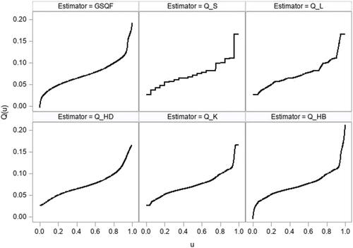
Table 5. Select estimated quantiles for spleen to brain weight ratios for n = 20 mice.

	u
Estimator	0.01	0.1	0.25	0.5	0.75	0.9	0.99	0.999
${\widehat{Q}}_{\widehat{\tau }}$	0.012	0.036	0.052	0.070	0.092	0.113	0.175	0.192
${\widehat{Q}}_S$	0.025	0.042	0.057	0.070	0.098	0.110	0.165	0.165
${\widehat{Q}}_L$	0.025	0.037	0.056	0.069	0.094	0.110	0.165	0.165
${\widehat{Q}}_H$	0.025	0.036	0.056	0.069	0.094	0.114	0.165	0.165
${\widehat{Q}}_{HD}$	0.026	0.038	0.054	0.070	0.091	0.120	0.162	0.165
${\widehat{Q}}_K$	0.025	0.039	0.055	0.070	0.090	0.110	0.165	0.165
${\widehat{Q}}_{HB}$	0.013	0.038	0.055	0.070	0.090	0.110	0.186	0.211

Table 6. 95% Percentile confidence intervals for the E(X) and VAR(X) based on each quantile estimator for spleen to brain weight ratios for n = 20 mice.

	E(X)		STD(X)
Estimator	lower	upper	lower	upper
${\widehat{Q}}_{\widehat{\tau }}$	0.059	0.089	0.020	0.046
${\widehat{Q}}_S$	0.061	0.088	0.018	0.043
${\widehat{Q}}_L$	0.061	0.090	0.020	0.044
${\widehat{Q}}_H$	0.061	0.089	0.020	0.044
${\widehat{Q}}_{HD}$	0.061	0.089	0.020	0.041
${\widehat{Q}}_K$	0.061	0.089	0.019	0.042
${\widehat{Q}}_{HB}$	0.060	0.089	0.019	0.047

8. Concluding remarks

In this note we introduced a new class of smooth estimators based on utilizing the sigmoidal approximation in place of the absolute value function in quantile estimation. Our two quantile function estimators were well behaved and were shown to have strong utility in univariate bootstrap smoothing resampling procedures. The theory for our estimators followed straightforward from classic M-estimation theory. Our future work will be to use this approach to develop generalized expectile regression framework.

Additional information

Funding

This work was supported by Roswell Park Cancer Institute and National Cancer Institute (NCI) grant P30CA016056, NRG Oncology Statistical and Data Management Center grant U10CA180822 and IOTN Moonshot grant U24CA232979-01. We wish to thank the reviewer for making important suggestions that greatly improved the presentation of our work.

References

- Abdous, B., and B. Remillard. 1995. Relating quantiles and expectiles under weighted-wymmetry. Annals of the Institute of Statistical Mathematics 47 (2):371–84. doi:10.1007/BF00773468.
- Abdous, B., and R. Theodorescu. 1992. Note on the spatial quantile of a random vector. Statistics & Probability Letters 13 (4):333–6. doi:10.1016/0167-7152(92)90043-5.
- Bassett, G., Jr., and R. Koenker. 1982. An empirical quantile function for linear models with i.i.d. errors. Journal of the American Statistical Association 77:407–15.
- Chen, C., and O. L. Mangasarian. 1995. Smoothing methods for convex inequalities and linear complementarity problems. Mathematical Programming 71 (1):51–69. doi:10.1007/BF01592244.
- Cheng, C. 1995. The Bernstein polynomial estimator of a smooth quantile function. Statistics & Probability Letters 24 (4):321–30. doi:10.1016/0167-7152(94)00190-J.
- Davison, A. C., and D. V. Hinkley. 1997. Bootstrap methods and their applications. New York: Cambridge University Press.
- Efron, B., and R. Tibshirani. 1993. An introduction to the bootstrap. New York: Chapman & Hall.
- Hampel, F., C. Hennig, and E. Ronchetti. 2011. A smoothing principle for the Huber and other location M-estimators. Computational Statistics & Data Analysis 55 (1):324–37. doi:10.1016/j.csda.2010.05.001.
- Harrell, F., and C. E. Davis. 1982. A new distribution-free quantile estimator. Biometrika 69 (3):635–40. doi:10.1093/biomet/69.3.635.
- Hutson, A. D. 2000. A composite quantile function estimator with applications in bootstrapping. Journal of Applied Statistics 27 (5):567–77. doi:10.1080/02664760050076407.
- Hutson, A. D. 2002. A semiparametric quantile function estimator for use in bootstrap estimation procedures. Statistics and Computing 12 (4):331–8. doi:10.1023/A:1020783911574.
- Hutson, A. D. 2018. Quantile planes without crossing via nonlinear programming. Computer Methods and Programs in Biomedicine 153:185–90. doi:10.1016/j.cmpb.2017.10.019.
- Hutson, A. D., and M. D. Ernst. 2000. The exact bootstrap mean and variance of an L-estimator. Journal of the Royal Statistical Society: Series B (Statistical Methodology) 62 (1):89–94. doi:10.1111/1467-9868.00221.
- Jones, M. C. 1994. Expectiles and M-quantiles are quantiles. Statistics & Probability Letters 20 (2):149–53. doi:10.1016/0167-7152(94)90031-0.
- Koenecker, R. 1993. When are expectiles percentiles? Econometric Theory 9:526–7.
- Mao, T., K. W. Ng, and T. Hu. 2015. Asymptotic expansions of generalized quantiles and expectiles for extreme risks. Probability in the Engineering and Informational Sciences 29 (3):309–27. doi:10.1017/S0269964815000017.
- Mudholkar, G. S., A. D. Hutson, and C. E. Marchetti. 2001. A simple Hermitian estimator of the quantile function. Journal of Nonparametric Statistics 13 (2):229–43. doi:10.1080/10485250108832851.
- Newey, W. K., and J. L. Powell. 1987. Asymmetric least squares estimation and testing. Econometrica 55 (4):819–47. doi:10.2307/1911031.
- Parzen, E. 1993. Change PP plot and continuous sample quantile function. Communications in Statistics - Theory and Methods 22 (12):3287–304. doi:10.1080/03610929308831216.
- Polansky, A. M. 1999. Upper Bounds on the True Coverage of Bootstrap Percentile Type Confidence Interval. The American Statistician 53:362–9.
- Polansky, A. M., and W. R. Schucany. 1997. Kernel smoothing to improve bootstrap confidence intervals. Journal of the Royal Statistical Society: Series B (Statistical Methodology) 59 (4):821–38. doi:10.1111/1467-9868.00099.
- Reiss, R.-D. 1980. Estimation of quantiles in certain nonparametric models. Annals of Mathematical Statists 8:87–105.
- Reiss, R.-D. 1989. Approximate distributions of order statistics: With applications to nonparametric statistics. New York: Springer-Verlag.
- Schmidt, M., G. Fung, and R. Rosales. 2007. Fast optimization methods for L1 regularization: A comparative study and two new approaches. In Machine learning: ECML 2007. Lecture notes in computer science, Vol. 4701, ed. J. N. Kok, J. Koronacki, R. L. Mantaras, S. Matwin, D. Mladenič, and A. Skowron. Berlin, Heidelberg: Springer.
- Serfling, R. J. 1980. Approximation theorems of mathematical statistics. New York: John Wiley & Sons.
- Shao, J., and D. Tu. 1995. The Jackknife and bootstrap. New York: Springer-Verlag.
- Sheather, S. J., and J. S. Marron. 1990. Kernel quantile estimators. Journal of the American Statistical Association 85 (410):410–6. doi:10.1080/01621459.1990.10476214.
- Stigler, S. M. 1977. Fractional order statistics, with applications. Journal of the American Statistical Association 72 (359):544–50. doi:10.1080/01621459.1977.10480611.
- Young, G. A. 1994. Bootstrap: More than a stab in the dark. Statistical Science 9 (3):382–415. doi:10.1214/ss/1177010383.