A multivariate adaptive control chart for simultaneously monitoring of the process parameters

Abstract

There have been some advances in multivariate control charts in recent years. This paper presents a new simultaneous scheme for monitoring both the mean and variability of a multivariate normal process in a single chart, which is developed by improving and modifying another recently proposed scheme. We not only propose a new control scheme but also make it adaptive by varying all control chart parameters. Our scheme, for the first time, considers the process variability in two forms: “covariance matrix” and “multivariate coefficient of variation (MCV)”. This scheme, again for the first time, considers simultaneous monitoring of the MCV with another process parameter (in our case, the mean vector). In addition, we develop a Markov chain model to compute the average run length and average time to signal values. We conduct extensive numerical analyses to measure the performance of the proposed scheme in two scenarios of process variability. At last, we present a numerical example by using a real dataset from a healthcare process to illustrate how the scheme can be implemented in practice.

Keywords:

• Markov chains
• Multivariate coefficient of variation
• Multivariate normal process parameters
• Simultaneous monitoring
• Single-chart monitoring
• Variable parameters control charts

1. Introduction

Process monitoring is performed to control the variability of the process to ensure that good quality products/services are delivered. Process control charts are the main tools for this purpose. They come in many forms and are being improved constantly by researchers. If the product/service consists of only one quality characteristic, univariate control charts are used, while in the case of more than one quality characteristic, multivariate control charts are employed. To be able to detect assignable causes which lead to small and moderate shifts in the process parameters (mean and variability), extra measures should be taken or some special control charts should be used. One way of doing this is by allowing the control charts’ parameters (sample size, sampling interval and control limits) to vary throughout process monitoring. There are different types of adaptive control charts but the best one allows all the chart’s parameters to vary (Sabahno, Amiri, and Castagliola 2021), namely, the variable parameters (VP) scheme. Chen (2007), Faraz et al. (2014) and Seif et al. (2016) were among the researchers who considered the VP adaptive feature on multivariate control charts. For other types of adaptive features used on multivariate control charts, one can refer to Aparisi, Jabaloyes, and Carrion (2001), Grigoryan and He (2005), Sabahno, Amiri, and Castagliola (2018a, 2018b), Aparisi and Haro (2003), and Lee and Khoo (2015). All of the above researchers used adaptive features on multivariate control charts in monitoring either the process mean or process variability.

Simultaneous monitoring of the process parameters (mean and variability) has been proven to reduce the false alarm rates and improve the performance of the monitoring procedure. In general, control charts for simultaneous monitoring can be divided into single-chart and double-chart (one for each parameter) schemes. Concerning multivariate control charts, in which two separate charts were used, one may refer to Reynolds and Cho (2006), Hawkins and Maboudou-Tchao (2008), and Zhang and Chang (2008). For researches in which single multivariate charts were used, one may refer to Khoo (2005), Zhang, Li, and Wang (2010), Wang, Yeh, and Li (2014) and Sabahno, Amiri, and Castagliola (2021). Concerning using adaptive features in simultaneous monitoring schemes, see Reynolds and Kim (2007), Reynolds and Cho (2011), and Sabahno, Castagliola, and Amiri (2020a, 2020b) and Sabahno, Amiri, and Castagliola (2021).

Sometimes the estimators for the mean and variability are not independent even though their independence is usually assumed. In these cases, the variability is measured in the form of the coefficient of variation (CV), which is simply computed by dividing the standard deviation by the mean. Monitoring the CV is mostly important in chemical and biological processes (Reed, Lynn, and Meade 2002) and also in the fields of materials engineering and manufacturing (Castagliola, Celano, and Psarakis 2011). For the examples of developing univariate control charts for monitoring the CV, please refer to Kang et al. (2007), Hong et al. (2008), Calzada and Scariano (2013), Castagliola et al. (2013a), and Zhang et al. (2014); and for adaptive based CV control charts to Castagliola et al. (2013b) and Khaw et al. (2017).

There are several definitions of multivariate coefficient of variation but the most commonly used one was defined by Voinov and Nikulin (1996). The first control chart for the MCV was introduced by Yeong et al. (2016). Adaptive features were later added to their scheme by Nguyen et al. (2019) and Khaw et al. (2018).

In monitoring the CV, the shift in the CV may change the relationship between the mean and the standard deviation. In this case, it is possible that the process mean goes out-of-control but the ratio of σ to μ is still in-control. Noor-ul-Amin, Tariq, and Hanif (2019) is the only research in the literature that considered simultaneous monitoring of the CV and the mean and it was for a univariate scheme. To the best of our knowledge, there is no such scheme for the multivariate case.

Sabahno, Amiri, and Castagliola (2021). proposed a new simultaneous scheme for monitoring the process mean vector and covariance matrix. They also added adaptive features and computed several performance measures using a Markov chain model. They, for the first time on SPC control charts, used a statistic to represent the process variation. However, the distribution of the said statistic increasingly loses its fitness for data with more than two quality characteristics.

In this research, we not only solve the abovementioned issue by suggesting a new statistic with a deterministic distribution, but our statistic can be used for MCV monitoring as well. In fact, this is the first research that simultaneously monitors the process mean and MCV. Our scheme is such that variation in two forms can be considered; Scenario 1: covariance matrix and Scenario 2: MCV. We also develop a new Markov chain model to compute the performance measures. Several numerical analyses and simulation runs will be conducted in the two mentioned variability scenarios. Based on a real data set from a health care process, at last, we show how the scheme can be implemented in practice.

The structure of this paper is as follows: In Sec. 2, the proposed multivariate control chart for simultaneous monitoring of the mean and variability is developed. The VP adaptive features are developed for the proposed scheme in Sec. 3. In Sec. 4, performance measures are derived using a Markov chain model. Numerical analyses are performed to examine the proposed scheme in Sec. 5. An illustrative example is presented in Sec. 6. Finally, concluding remarks are given in Sec. 7.

2. Multivariate control charts for a simultaneous monitoring of the mean and variability

Sabahno, Amiri, and Castagliola (2021) developed a novel scheme to simultaneously monitor the mean and variability of multivariate normal processes. However, the distribution they used for the process variability statistic, loses its fitness for cases with more than two dimensions (quality characteristics), as when the dimension increases, the less accurate their scheme becomes. They used the $W_i=\frac{(n-1){\left|{\mathbf{S}}_i\right|}^{1/p}}{{\left|{\mathbf{\Sigma }}_0\right|}^{1/p}}$ statistic (its parameters will be introduced later on in this section) for monitoring the variability, whose distribution when $p>2$ is unknown, but it approximatelly follows the gamma $\Gamma (a,b)$ distribution with parameters $a=p(n-p)/2$ and $b=\frac{2}{p}{(1-\frac{(p-1)(p-2)}{2n})}^{-1/p}.$ As mentioned before, as p (the number of quality charactristics) increases, the $W_i$ statistic deviates more from this gamma distribution (Gnanadesikan and Gupta 1970).

Wijsman (1957) has shown that letting $T_i{}^2=n{\overline{\mathit{X}}}_i{}^T{\mathbf{S}}_i{}^{-1}{\overline{\mathit{X}}}_i,$ gives (1) $${\Upsilon }_i=\frac{T_i{}^2}{n-1}.\frac{n-p}{p}:F_{p,n-p,{\delta }_0}(x),$$(1) where $F_{p,n-p,{\delta }_0}(\cdot )$ is the non-central Fisher distribution with p and n − p degrees of freedom and non-centrality parameter ${\delta }_0=n{\mathbf{\mu }}_0{}^T{\mathbf{\Sigma }}_0{}^{-1}{\mathbf{\mu }}_0$ when the process is in-control, n is the sample (subgroup) size, ${\overline{\mathit{X}}}_i$ is the ith sample mean vector, and ${\mathbf{S}}_i$ is the ith sample covariance matrix.

A transformation of the statistic ${\Upsilon }_i$ has been used by Yeong et al. (2016) for monitoring the multivariate coefficient of variation. When the in-control process parameters (${\mathbf{\mu }}_0$ and ${\mathbf{\Sigma }}_0$) are known, the population MCV is computed as ${\gamma }_0={({\mathbf{\mu }}_0{}^T{\mathbf{\Sigma }}_0{}^{-1}{\mathbf{\mu }}_0)}^{-\frac{1}{2}},$ while for sample i, the sample MCV is obtained as ${\tilde{\gamma }}_i={({\overline{\mathbf{X}}}_i{}^T{\mathbf{S}}_i{}^{-1}{\overline{\mathbf{X}}}_i)}^{-\frac{1}{2}}.$

We use ${\Upsilon }_i$ instead of Sabahno, Amiri, and Castagliola (2021)’s method, which is based on the generalized variance statistic for monitoring the process variability. The ${\Upsilon }_i$ statistic, if the process mean and variability are not independant, can be used for monitoring the MCV (${\gamma }_0$) as well (it was primarily used for that purpose in control charts). However, we want to broaden its application for all kinds of variability and not only for the MCV. Substituting $n{\tilde{\gamma }}_i{}^{-2}$ for $T_i{}^2$ in Eq. (1)(1) $${\Upsilon }_i=\frac{T_i{}^2}{n-1}.\frac{n-p}{p}:F_{p,n-p,{\delta }_0}(x),$$(1) , gives $\frac{n{\tilde{\gamma }}_i{}^{-2}}{n-1}.\frac{n-p}{p}:F_{p,n-p,{\delta }_0}(x),$ where ${\delta }_0=n{\gamma }_0{}^{-2}.$ In this way, ${\Upsilon }_i$ in Eq. (1)(1) $${\Upsilon }_i=\frac{T_i{}^2}{n-1}.\frac{n-p}{p}:F_{p,n-p,{\delta }_0}(x),$$(1) can be used for monitoring the MCV.

To monitor the process mean, the Hotelling’s $T^{2\prime }$ statistic (note that the small prime in $T^{2\prime }$ is to distinguish it from the $T_i{}^2$ statistic in Eq. (1)(1) $${\Upsilon }_i=\frac{T_i{}^2}{n-1}.\frac{n-p}{p}:F_{p,n-p,{\delta }_0}(x),$$(1) is computed for each subgroup $i=1,2,\dots ,$ as (2) $$T_i{}^{2\prime }=n{({\overline{\mathbf{X}}}_i\mathbf{-}{\mathbf{\mu }}_0)}^T{\left({\mathbf{\Sigma }}_0\right)}^{-1}({\overline{\mathbf{X}}}_i\mathbf{-}{\mathbf{\mu }}_0),$$(2) where $T_i{}^{2\prime }$∼${\chi }^2(p),$ i.e., a chi-square distribution with p degrees of freedom when the process is in-control and p is the number of quality characteristics.

To monitor the mean and variability simultaneously, we use the following transformations of $T^{2\prime }$ and ${\Upsilon }_i:$ (3) $$M_i={\Phi }^{-1}\left[H_p(T_i{}^{2\prime })\right]\sim N(0,1),i=1,2,\dots ,$$(3) and (4) $$C{V}_i={\Phi }^{-1}\left[F_{p,n-p,\delta }({\Upsilon }_i)\right]\sim N(0,1),i=1,2,\dots ,$$(4) where $\Phi (\cdot )$ is the standard normal cumulative distribution function, $H_p(\cdot )$ is the chi-square cumulative distribution function with p degrees of freedom and $F_{p,n-p,\delta }(\cdot )$ denotes the Fisher cumulative distribution function with p and n − p degrees of freedom and non-centrality parameter $\delta .$

Then, we use the following max-type statistic: (5) $$M{V}_i=\mathit{\text{max}}\left\{\left|M_i\right|,\left|C{V}_i\right|\right\}.$$(5)

By assuming the independence of $M_i$ and $C{V}_i,$ the upper control limit (UCL) of this chart can be obtained as follows: $$\begin{array}{c}P(M{V}_i\le \mathit{\text{UCL}})=P(\mathit{\text{max}}\left\{\left|M_i\right|,\left|C{V}_i\right|\right\}\le \mathit{\text{UCL}})\\ =P(-\mathit{\text{UCL}}\le M_i\le \mathit{\text{UCL}})P(-\mathit{\text{UCL}}\le C{V}_i\le \mathit{\text{UCL}})\\ =(2\Phi (\mathit{\text{UCL}})-1)(2\Phi (\mathit{\text{UCL}})-1)={(2\Phi (\mathit{\text{UCL}})-1)}^2.\end{array}$$

As $P(M{V}_i\le \mathit{\text{UCL}})=1-\alpha ,$ then (6) $$\mathit{\text{UCL}}={\Phi }^{-1}\left[\frac{\sqrt{1-\alpha }+1}{2}\right],$$(6) where $\alpha$ is the probability of a Type-I error.

We have confirmed via simulation runs that Eq. (6)(6) $$\mathit{\text{UCL}}={\Phi }^{-1}\left[\frac{\sqrt{1-\alpha }+1}{2}\right],$$(6) provides a good approximation of UCL for this control chart.

3. Simultaneous monitoring scheme with variable parameters control chart

For a variable parameters (VP) control chart, all the chart’s parameters are variable. In this paper, we assume that there are two different (i) sample sizes ($n_s:s\in \left\{1,2\right\}$ with $n_1<n_2),$ (ii) sampling intervals ($t_s:s\in \left\{1,2\right\}$ with $t_2<t_1)$ and (iii) Type-I error probabilities $({\alpha }_s:s\in \left\{1,2\right\}$ with ${\alpha }_1<{\alpha }_2).$

Since our max-type control chart is one-sided, we also assume that there are two upper control limits ${\mathit{\text{UCL}}}_1$ (related to ${\alpha }_1$) and ${\mathit{\text{UCL}}}_2$ (related to ${\alpha }_2$), and two upper warning limits ${\mathit{\text{UWL}}}_1$ and ${\mathit{\text{UWL}}}_2,$ satisfying ${\mathit{\text{UWL}}}_1<{\mathit{\text{UCL}}}_1$ and ${\mathit{\text{UWL}}}_2<{\mathit{\text{UCL}}}_2.$

The VP strategy for choosing the next sampling scheme works as follows:

• If $M{V}_i\in [0,\mathit{\text{UWL}}],$ the process is declared as in-control and the parameters for the next sample must be ${\Omega }_1=(n_1,t_1,{\mathit{\text{UCL}}}_1,{\mathit{\text{UWL}}}_1),$ i.e., the small sample size, long sampling interval and higher control (UCL) and warning (UWL) limits.

• If $M{V}_i\in (\mathit{\text{UWL}},\mathit{\text{UCL}}],$ the process is also declared as in-control but the parameters for the next sample must be ${\Omega }_2=(n_2,t_2,{\mathit{\text{UCL}}}_2,{\mathit{\text{UWL}}}_2),$ i.e., the large sample size, short sampling interval and lower control (UCL) and warning (UWL) limits.

• If $M{V}_i\in (\mathit{\text{UCL}},\infty ),$ the process is declared as out-of-control and corrective actions have to be taken.

In the VP scheme, the following equations should be satisfied: (7) $$\mathit{\text{ASS}}=n_1{P}_0+n_2(1-P_0),$$(7) (8) $$\mathit{\text{ASI}}=t_1{P}_0+t_2(1-P_0),$$(8) (9) $$\mathit{\text{ATE}}={\alpha }_1{P}_0+{\alpha }_2(1-P_0),$$(9)

Note that ASS is the average sample size, ASI is the average sampling interval and ATE is the average Type-I error, where $P_0$ is the probability $M{V}_i$ of being in the safe state (${\Omega }_1$) while the process is in-control, i.e., (10) $$\begin{array}{c}{P}_0=\frac{P(M{V}_i\le \mathit{\text{UWL}})}{P(M{V}_i\le \mathit{\text{UCL}})}=\frac{P(\mathit{\text{max}}\left\{\left|M_i\right|,\left|C{V}_i\right|\right\}\le \mathit{\text{UWL}})}{P(\mathit{\text{max}}\left\{\left|M_i\right|,\left|C{V}_i\right|\right\}\le \mathit{\text{UCL}})}\\ =\frac{P(\left|M_i\right|\le \mathit{\text{UWL}})P(\left|C{V}_i\right|\le \mathit{\text{UWL}})}{P(\left|M_i\right|\le \mathit{\text{UCL}})P(\left|C{V}_i\right|\le \mathit{\text{UCL}})}=\frac{{[2\Phi (\mathit{\text{UWL}})-1]}^2}{{[2\Phi (\mathit{\text{UCL}})-1]}^2}\end{array}$$(10)

By solving Eqs. (7)–(10) simultaneously, we can obtain the chart’s parameters as follows: (11) $${\alpha }_2=\frac{\mathit{\text{ATE}}(n_1-n_2)-{\alpha }_1(\mathit{\text{ASS}}-n_2)}{n_1-\mathit{\text{ASS}}},$$(11) (12) $$t_1=\frac{\mathit{\text{ASI}}(n_1-n_2)-t_2(n_1-\mathit{\text{ASS}})}{\mathit{\text{ASS}}-n_2},$$(12) (13) $${\mathit{\text{UWL}}}_s={\Phi }^{-1}\left(\frac{(2\Phi ({\mathit{\text{UCL}}}_s)-1)\sqrt{P_0}+1}{2}\right),$$(13) where $P_0$ is obtained from Eq. (7)(7) $$\mathit{\text{ASS}}=n_1{P}_0+n_2(1-P_0),$$(7) as $P_0=\frac{\mathit{\text{ASS}}-n_2}{n_1-n_2}.$

4. Performance measures

In general, there are two types of performance measures, i.e., initial-state and steady-state performance measures. In the initial-state performance measures, it is assumed that the process is out-of-control at the beginning of process monitoring. On the contrary, in the steady-state performance measures, the assumption is that the process is in-control at the beginning of process monitoring but it will become out-of-control later on. In the steady-state performance measures, an additional complexity will be added to the model, that is approximating the time that the process goes out-of-control. In this paper, we only consider the initial-state performance measures, as they are sufficient for our performance measure agenda.

We use a Markov chain model to derive the performance measures. In an initial-state condition, this approach requires the definition of the following three states for the proposed control scheme:

• State 1: $M{V}_i\in \left[0,\mathit{\text{UWL}}\right],$

• State 2:$M{V}_i\in (\mathit{\text{UWL}},\mathit{\text{UCL}}],$

• State 3: $M{V}_i\in (\mathit{\text{UCL}},\infty ).$

The first two states are transient, while the third one is absorbing. The Markov chain transition probability matrix P corresponding to the VP chart is equal to $$\mathbf{P}=\left[\begin{array}{ccc}{p}_{11}& p_{12}& p_{13}\\ p_{21}& p_{22}& p_{23}\\ p_{31}& p_{32}& p_{33}\end{array}\right],$$ where $p_{\mathit{\text{ij}}}$ is the probability of transitioning from state i to state j. Note that for a steady-state performance measure, we have more states and consequently the dimension of the transition probability matrix is larger.

Since it is mathematically very complicated (if not impossible) to show the independence of $M_i$ and $C{V}_i$ (we need them to be independent to be able to compute the following probabilities), we have confirmed their independence via simulation runs (by comparing the performances computed by simulation and the following Markov chain methods), and consequently, concluded that $M_i$ and $C{V}_i$ are somewhat independent.

Therefore, the transient state probabilities $p_{11},$ $p_{12},$ $p_{21}$ and $p_{22}$ for the proposed multivariate max-type chart are equal to (14) $$\begin{array}{c}{p}_{s1}=P(M{V}_i\le \mathit{\text{UWL}})=P(\mathit{\text{max}}\left\{\left|M_i\right|,\left|C{V}_i\right|\right\}\le \mathit{\text{UWL}})\\ =P(-\mathit{\text{UWL}}\le M_i\le \mathit{\text{UWL}})P(-\mathit{\text{UWL}}\le C{V}_i\le \mathit{\text{UWL}}),\end{array}$$(14) (15) $$\begin{array}{c}{p}_{s2}=P(\mathit{\text{UWL}}<M{V}_i\le \mathit{\text{UCL}})=P(\mathit{\text{UWL}}<\mathit{\text{max}}\left\{\left|M_i\right|,\left|C{V}_i\right|\right\}\le \mathit{\text{UCL}})\\ =P(-\mathit{\text{UCL}}\le M_i\le \mathit{\text{UCL}})P(-\mathit{\text{UCL}}\le C{V}_i\le \mathit{\text{UCL}})\\ -P(-\mathit{\text{UWL}}\le M_i\le \mathit{\text{UWL}})P(-\mathit{\text{UWL}}\le C{V}_i\le \mathit{\text{UWL}}).\end{array}$$(15)

Concerning the other transition probabilities, we simply have $p_{13}=1-p_{11}-p_{12} ,$$p_{23}=1-p_{21}-p_{22},$ $p_{31}=p_{32}=0$ and $p_{33}=1.$

As it can be seen, Eqs. (14)(14) $$\begin{array}{c}{p}_{s1}=P(M{V}_i\le \mathit{\text{UWL}})=P(\mathit{\text{max}}\left\{\left|M_i\right|,\left|C{V}_i\right|\right\}\le \mathit{\text{UWL}})\\ =P(-\mathit{\text{UWL}}\le M_i\le \mathit{\text{UWL}})P(-\mathit{\text{UWL}}\le C{V}_i\le \mathit{\text{UWL}}),\end{array}$$(14) and (15)(15) $$\begin{array}{c}{p}_{s2}=P(\mathit{\text{UWL}}<M{V}_i\le \mathit{\text{UCL}})=P(\mathit{\text{UWL}}<\mathit{\text{max}}\left\{\left|M_i\right|,\left|C{V}_i\right|\right\}\le \mathit{\text{UCL}})\\ =P(-\mathit{\text{UCL}}\le M_i\le \mathit{\text{UCL}})P(-\mathit{\text{UCL}}\le C{V}_i\le \mathit{\text{UCL}})\\ -P(-\mathit{\text{UWL}}\le M_i\le \mathit{\text{UWL}})P(-\mathit{\text{UWL}}\le C{V}_i\le \mathit{\text{UWL}}).\end{array}$$(15) are both sums of products $P(m_1\le M_i\le m_2)$ by $P(c{v}_1\le C{V}_i\le c{v}_2),$ where $m_1,m_2,$$c{v}_1\mathrm{ }\text{and}\mathrm{ }\mathrm{c}{v}_2$ stand for +/−UWL and +/−UCL. In general, these terms can be evaluated using Eqs. (18)(18) $$P(m_1\le M_i\le m_2)=H_{p,\lambda }(H_p^{-1}(\Phi (m_2))\times (1/{\tau }_1))-H_{p,\lambda }(H_p^{-1}(\Phi (m_1))\times (1/{\tau }_1)).$$(18) and (20)(20) $$\begin{array}{l}P(c{v}_1\le C{V}_i\le c{v}_2)=\\ F_{{}_{p,n-p,{\delta }_1}}(F_{{}_{p,n-p,{\delta }_0}}^{-1}(\Phi (c{v}_2)))-F_{{}_{p,n-p,{\delta }_1}}(F_{{}_{p,n-p,{\delta }_0}}^{-1}(\Phi (c{v}_1))).\end{array}$$(20) when the process is out-of-control and using Eqs. (19)(19) $$P(m_1\le M_i\le m_2)=H_p(H_p^{-1}(\Phi (m_2)))-H_p(H_p^{-1}(\Phi (m_1)))=\Phi (m_2)-\Phi (m_1).$$(19) and (21)(21) $$\begin{array}{c}P(c{v}_1\le C{V}_i\le c{v}_2)=F_{{}_{p,n-p,{\delta }_0}}(F_{{}_{p,n-p,{\delta }_0}}^{-1}(\Phi (c{v}_2)))-F_{{}_{p,n-p,{\delta }_0}}(F_{{}_{p,n-p,{\delta }_0}}^{-1}(\Phi (c{v}_1)))\\ =\Phi (c{v}_2)-\Phi (c{v}_1).\end{array}$$(21) when the process is in-control. Let us first derive Eqs. (18)(18) $$P(m_1\le M_i\le m_2)=H_{p,\lambda }(H_p^{-1}(\Phi (m_2))\times (1/{\tau }_1))-H_{p,\lambda }(H_p^{-1}(\Phi (m_1))\times (1/{\tau }_1)).$$(18) and (19)(19) $$P(m_1\le M_i\le m_2)=H_p(H_p^{-1}(\Phi (m_2)))-H_p(H_p^{-1}(\Phi (m_1)))=\Phi (m_2)-\Phi (m_1).$$(19) for $P(m_1\le M_i\le m_2).$ We have (16) $$\begin{array}{c}P(m_1\le M_i\le m_2)=P(m_1\le {\Phi }^{-1}\left[H_p(T_i{}^{2\prime })\right]\le m_2)\\ =P(\Phi (m_1)\le \left[H_p(T_i{}^{2\prime })\right]\le \Phi (m_2))\\ =P(H_p^{-1}(\Phi (m_1))\le T_i{}^{2\prime }\le H_p^{-1}(\Phi (m_2))).\end{array}$$(16)

As in Sabahno, Amiri, and Castagliola (2021), in an out-of-control case, we have the non-centrality parameter $\lambda$ equal to (17) $$\lambda =n_s{({\mathbf{\mu }}_1-{\mathbf{\mu }}_0)}^T{\left({\mathbf{\Sigma }}_1\right)}^{-1}({\mathbf{\mu }}_1-{\mathbf{\mu }}_0).$$(17)

Note that the non-centrality parameter $\lambda$ can be influenced by both the mean vector and the variance-covariance matrix shifts, however, there should be a mean vector shift first in order for the variance-covariance shift to be effective.

In this paper, for simplicity and also to be able to keep track of the coefficient of variability in the scheme, we assume that ${\mathbf{\Sigma }}_1={\tau }_1{\mathbf{\Sigma }}_0,$ and therefore, $\lambda$ changes to $\lambda =n_s{({\mathbf{\mu }}_1-{\mathbf{\mu }}_0)}^T{({\tau }_1{\mathbf{\Sigma }}_0)}^{-1}({\mathbf{\mu }}_1-{\mathbf{\mu }}_0).$

As a result, we have (18) $$P(m_1\le M_i\le m_2)=H_{p,\lambda }(H_p^{-1}(\Phi (m_2))\times (1/{\tau }_1))-H_{p,\lambda }(H_p^{-1}(\Phi (m_1))\times (1/{\tau }_1)).$$(18)

If we monitor the MCV for variability, ${\tau }_2$ is obtained as follows: $${\tau }_2=\frac{{\gamma }_1}{{\gamma }_0}=\frac{{\left({\mathbf{\mu }}_1{}^T{({\tau }_1{\mathbf{\Sigma }}_0)}^{-1}{\mathbf{\mu }}_1\right)}^{-\frac{1}{2}}}{{\left({\mathbf{\mu }}_0{}^T{\mathbf{\Sigma }}_0{}^{-1}{\mathbf{\mu }}_0\right)}^{-\frac{1}{2}}}\Rightarrow {\tau }_1=\frac{{\tau }_2^2\left({\mathbf{\mu }}_1{}^T{\mathbf{\Sigma }}_0{}^{-1}{\mathbf{\mu }}_1\right)}{\left({\mathbf{\mu }}_0{}^T{\mathbf{\Sigma }}_0{}^{-1}{\mathbf{\mu }}_0\right)}.$$

When the process is in-control, i.e., $\lambda =0$ and ${\tau }_1={\tau }_2=1,$ Eq. (18)(18) $$P(m_1\le M_i\le m_2)=H_{p,\lambda }(H_p^{-1}(\Phi (m_2))\times (1/{\tau }_1))-H_{p,\lambda }(H_p^{-1}(\Phi (m_1))\times (1/{\tau }_1)).$$(18) reduces to (19) $$P(m_1\le M_i\le m_2)=H_p(H_p^{-1}(\Phi (m_2)))-H_p(H_p^{-1}(\Phi (m_1)))=\Phi (m_2)-\Phi (m_1).$$(19)

Similarly, for $P(c{v}_1\le C{V}_i\le c{v}_2),$ we have $$\begin{array}{c}P(c{v}_1\le C{V}_i\le c{v}_2)=P(c{v}_1\le {\Phi }^{-1}\left[F_{p,n-p,\delta }({\Upsilon }_i)\right]\le c{v}_2)\\ =P(\Phi (c{v}_1)\le \left[F_{p,n-p,\delta }({\Upsilon }_i)\right]\le \Phi (c{v}_2))\\ =P(F_{p,n-p,{\delta }_0}^{-1}(\Phi (c{v}_1))\le {\Upsilon }_i\le F_{p,n-p,{\delta }_0}^{-1}(\Phi (c{v}_2)))\\ \mathrm{ }\end{array}$$

To obtain the distribution of ${\Upsilon }_i$ when the process is out-of-control, we have (20) $$\begin{array}{l}P(c{v}_1\le C{V}_i\le c{v}_2)=\\ F_{{}_{p,n-p,{\delta }_1}}(F_{{}_{p,n-p,{\delta }_0}}^{-1}(\Phi (c{v}_2)))-F_{{}_{p,n-p,{\delta }_1}}(F_{{}_{p,n-p,{\delta }_0}}^{-1}(\Phi (c{v}_1))).\end{array}$$(20)

When the process is in-control, i.e., ${\delta }_1={\delta }_0,$ Eq. (20)(20) $$\begin{array}{l}P(c{v}_1\le C{V}_i\le c{v}_2)=\\ F_{{}_{p,n-p,{\delta }_1}}(F_{{}_{p,n-p,{\delta }_0}}^{-1}(\Phi (c{v}_2)))-F_{{}_{p,n-p,{\delta }_1}}(F_{{}_{p,n-p,{\delta }_0}}^{-1}(\Phi (c{v}_1))).\end{array}$$(20) reduces to (21) $$\begin{array}{c}P(c{v}_1\le C{V}_i\le c{v}_2)=F_{{}_{p,n-p,{\delta }_0}}(F_{{}_{p,n-p,{\delta }_0}}^{-1}(\Phi (c{v}_2)))-F_{{}_{p,n-p,{\delta }_0}}(F_{{}_{p,n-p,{\delta }_0}}^{-1}(\Phi (c{v}_1)))\\ =\Phi (c{v}_2)-\Phi (c{v}_1).\end{array}$$(21)

One can easily compute Eqs. (14)(14) $$\begin{array}{c}{p}_{s1}=P(M{V}_i\le \mathit{\text{UWL}})=P(\mathit{\text{max}}\left\{\left|M_i\right|,\left|C{V}_i\right|\right\}\le \mathit{\text{UWL}})\\ =P(-\mathit{\text{UWL}}\le M_i\le \mathit{\text{UWL}})P(-\mathit{\text{UWL}}\le C{V}_i\le \mathit{\text{UWL}}),\end{array}$$(14) and (15)(15) $$\begin{array}{c}{p}_{s2}=P(\mathit{\text{UWL}}<M{V}_i\le \mathit{\text{UCL}})=P(\mathit{\text{UWL}}<\mathit{\text{max}}\left\{\left|M_i\right|,\left|C{V}_i\right|\right\}\le \mathit{\text{UCL}})\\ =P(-\mathit{\text{UCL}}\le M_i\le \mathit{\text{UCL}})P(-\mathit{\text{UCL}}\le C{V}_i\le \mathit{\text{UCL}})\\ -P(-\mathit{\text{UWL}}\le M_i\le \mathit{\text{UWL}})P(-\mathit{\text{UWL}}\le C{V}_i\le \mathit{\text{UWL}}).\end{array}$$(15) using the terms $P(m_1\le M_i\le m_2)$ and $P(c{v}_1\le C{V}_i\le c{v}_2),$ by replacing$m_1,m_2,$$c{v}_1\mathrm{ }\text{and}\mathrm{ }\mathrm{c}{v}_2$ in Eqs. (18)–(21) with ±UWL and ±UCL.

Finally, the performance measures, i.e., the average run length (ARL) and average time to signal (ATS) can be computed. For an adaptive scheme, there could be additional performance measures based on the number of observations to signal and the number of switches between the in-control states before a signal is issued, but these measures will not be considered. Since time is the most important element in process monitoring schemes, ATS is by far the most important performance measure that should not be ignored.

Thus, for performance measures, we have (22) $$\text{ARL}={\mathbf{b}}^T{\left(\mathbf{I}\mathbf{-}\mathbf{Q}\right)}^{-1}\mathbf{1},$$(22) (23) $$\text{ATS}={\mathbf{b}}^T{\left(\mathbf{I}\mathbf{-}\mathbf{Q}\right)}^{-1}\mathbf{t},$$(23) where ${\mathbf{b}}^{\mathbf{T}}$ = ($b_1,b_2)$ is the vector of starting probabilities such that $b_1+b_2=1,$ I is the identity matrix of order 2, $\mathbf{Q}$ is a $2\times 2$ transition probability matrix for the transient states, 1 is a $2\times 1$ unit column vector, $\mathbf{t}={(t_1,t_2)}^T$ is the vector of sampling intervals.

In the beginning, when the process is assumed to be in-control $({\mathbf{\mu }}_1={\mathbf{\mu }}_0\&{\tau }_1=1),$ $b_1$ and $b_2$ are obtained as follows: $$b_1=\frac{p_{11}}{p_{11}+p_{12}},$$ $$b_2=\frac{p_{22}}{p_{21}+p_{22}}.$$

5. Numerical analyses

To analyze the performance of the developed simultaneous scheme, we consider two scenarios.

• Scenario 1: In the first scenario, ${\mathbf{\mu }}_1$ can be any vector and as mentioned in the previous section, we have ${\mathbf{\Sigma }}_1={\tau }_1{\mathbf{\Sigma }}_0.$

• Scenario 2: In this scenario, ${\mathbf{\mu }}_1$ again can be any vector and in addition, we assume that the variation occurs in the form of the MCV. Therefore, we only make assumptions about the shifted values of ${\mathbf{\mu }}_0$ and ${\gamma }_0,$ i.e. ${\mathbf{\mu }}_1$ and ${\gamma }_1={\tau }_2{\gamma }_0.$

5.1. First scenario

We will conduct analyses for cases with p = 2 and 4. For all of our analyses, we assume that ${\alpha }_1$ = 0.0045, ATE = 0.005 (which results in ${\mathit{\text{UCL}}}_1$= 3.0547), in-control ASS = 10 and in-control ASI = 1.

For the case p = 2: $${\mathbf{\Sigma }}_0=\left[\begin{array}{cc}1& 0.5\\ 0.5& 1\end{array}\right],{\mathbf{\Sigma }}_1=\left[\begin{array}{cc}{\tau }_1& 0.5{\tau }_1\\ 0.5{\tau }_1& {\tau }_1\end{array}\right],{\tau }_1\in \left\{0.25,0.5,1,1.5,2\right\}$$ $${\mathbf{\mu }}_1-{\mathbf{\mu }}_0\in \{(0,0),(0.1,0),(0.1,0.1),(0.5,0),(0.5,0.5),(1,1),(2,2)\}.$$

The results of this analysis which are presented in Table 1 show that:

Table 1. ARL and ATS values for Scenario 1 (mean vector and covariance matrix shift) with p = 2.

	$t_2=0.01,t_1=3.48$ $n_1=5,n_2=12$ ${\mathit{\text{UWL}}}_1=0.7279,{\mathit{\text{UWL}}}_2=0.7276$	$t_2=0.01,t_1=1.99$ $n_1=8,n_2=12$ ${\mathit{\text{UWL}}}_1=1.0483,{\mathit{\text{UWL}}}_2=1.0476$	$t_2=0.1,t_1=1.9$ $n_1=5,n_2=15$ ${\mathit{\text{UWL}}}_1=1.0483,{\mathit{\text{UWL}}}_2=1.0476$	$t_2=0.1,t_1=1.36$ $n_1=8,n_2=15$ ${\mathit{\text{UWL}}}_1=1.4161,{\mathit{\text{UWL}}}_2=1.4136$	$t_2=0.5,t_1=2.25$ $n_1=5,n_2=12$ ${\mathit{\text{UWL}}}_1=0.7279,{\mathit{\text{UWL}}}_2=0.7276$
$({\mathbf{\mu }}_{\mathbf{1}}\mathbf{-}{\mathbf{\mu }}_{\mathbf{0}})$	${\tau }_1=0.25$
(0,0)’	11.2364, 1.7744	11.1929, 2.3832	6.5519, 2.1855	6.7265, 2.7485	11.2364, 6.4576
$(0,0.1)\prime ,$ $(0.1,0)\prime$	8.7016, 1.5016	8.6675, 1.8499	5.1035, 1.8722	5.2125, 2.1675	8.7016, 5.0652
$(0.1,0.1)\prime$	7.0112, 1.3018	6.9754, 1.4875	4.1891, 1.6592	4.2580, 1.8057	7.0112, 4.1276
$(0,0.5)\prime ,$ $(0.5,0)\prime$	3.2043, 1.1065	3.2271, 1.0585	2.3087, 1.3756	2.3246, 1.2509	3.2043, 2.1448
$(0.5,0.5)\prime$	2.1478, 1.0514	2.2032, 1.0201	1.8082, 1.2211	1.8425, 1.1275	2.1478, 1.5941
$(1,1)\prime$	1.2866, 1.0030	1.2550, 1.0026	1.4730, 1.0496	1.3478, 1.0348	1.2866, 1.1434
$(2,2)\prime$	1.0003,1	1,1	1.0006, 1.0001	1,1	1.0003, 1.0002
$({\mathbf{\mu }}_{\mathbf{1}}\mathbf{-}{\mathbf{\mu }}_{\mathbf{0}})$	${\tau }_1=0.5$
(0,0)’	85.3977, 62.5239	87.3226, 68.5158	71.1606, 56.8719	76.2526, 65.6741	85.3977, 73.8453
$(0,0.1)\prime ,$ $(0.1,0)\prime$	66.4301, 43.3671	68.3563, 49.0857	51.6181, 37.9231	56.3418, 45.8370	66.4301, 54.7821
$(0.1,0.1)\prime$	51.7563, 29.0740	53.3518, 34.1436	37.7474, 24.8804	41.5261, 31.3924	51.7563, 40.3006
$(0,0.5)\prime ,$ $(0.5,0)\prime$	14.2531, 2.4280	14.1903, 3.2074	8.0257, 2.7271	8.1448, 3.3215	14.2531, 8.2808
$(0.5,0.5)\prime$	7.8520, 1.3789	7.7668, 1.5306	4.6022, 1.8159	4.5868, 1.8657	7.8520, 4.5828
$(1,1)\prime$	1.4393,1.0108	1.4467, 1.0050	1.4982, 1.0775	1.4598, 1.050	1.4393, 1.2229
$(2,2)\prime$	1.0041,1	1,1	1.0071, 1.0007	1, 1	1.0041, 1.0020
$({\mathbf{\mu }}_{\mathbf{1}}\mathbf{-}{\mathbf{\mu }}_{\mathbf{0}})$	${\tau }_1=1$
(0,0)’	200,200	200,200	200,200	200,200	200,200
$(0,0.1)\prime$ , $(0.1,0)\prime$	186.4751, 184.921	186.9714, 185.68	184.8480, 183.6981	185.9221, 185.0815	186.4751, 185.6902
$(0.1,0.1)\prime$	181.8345,179.486	182.596, 180.64	179.3004, 177.5987	180.9189, 179.6688	181.8345, 180.6482
$(0,0.5)\prime ,$ $(0.5,0)\prime$	14.1240 6.8366	14.388,7.799	10.6323, 6.1225	11.3108, 7.4121	14.1240, 10.4435
$(0.5,0.5)\prime$	12.5053,4.6590	12.6627,5.5469	9.0785, 4.4269	9.5489, 5.4987	12.5053, 8.5425
$(1,1)\prime$	1.6223,1.0453	1.6097,1.0248	1.5972, 1.1514	1.5492, 1.1030	1.6223, 1.3309
$(2,2)\prime$	1.0155,1.0002	1.0007,1	1.0272, 1.0028	1.0010, 1.0001	1.0155, 1.0078
$({\mathbf{\mu }}_{\mathbf{1}}\mathbf{-}{\mathbf{\mu }}_{\mathbf{0}})$	${\tau }_1=1.5$
(0,0)’	46.9896, 35.5238	46.7537, 37.0364	45.5076, 36.7755	45.2870, 38.7129	46.9896, 41.1988
$(0,0.1)\prime ,$ $(0.1,0)\prime$	47.6602, 37.1952	47.3946, 38.5330	46.5296, 38.5179	46.2169, 40.1904	47.6602, 42.3749
$(0.1,0.1)\prime$	51.6313, 41.7440	51.3506, 42.9872	50.7788, 43.1912	50.4067, 44.7042	51.6313, 46.6377
$(0,0.5)\prime$ , $(0.5,0)\prime$	8.2461, 4.8202	8.3148, 5.1883	7.1033, 4.6752	7.3296, 5.2215	8.2461, 6.5159
$(0.5,0.5)\prime$	8.0936, 4.4613	8.1562, 4.8470	6.9158, 4.3686	7.1333, 4.9263	8.0936, 6.2591
$(1,1)\prime$	1.6607, 1.0840	1.6442, 1.0711	4.3686, 1.1981	1.5888, 1.1612	1.6607, 1.3694
$(2,2)\prime$	1.0251, 1.0004	1.0034,1	1.0439, 1.0051	1.0048, 1.0005	1.0251, 1.0127
$({\mathbf{\mu }}_{\mathbf{1}}\mathbf{-}{\mathbf{\mu }}_{\mathbf{0}})$	${\tau }_1=2$
(0,0)’	17.0587, 9.8238	17.0103, 10.6484	15.8414, 10.3311	15.9004, 11.4868	17.0587, 13.4047
$(0,0.1)\prime ,$ $(0.1,0)\prime$	17.6107, 10.6280	17.5318, 11.4215	16.6456, 11.2560	16.6252, 12.3496	17.6107, 14.0841
$(0.1,0.1)\prime$	18.9642, 11.9951	18.8606, 12.7901	18.1854, 12.7603	18.1000, 13.8327	18.9642, 15.4445
$(0,0.5)\prime ,$ $(0.5,0)\prime$	5.7840, 3.3785	5.7977, 3.6013	5.2340, 3.4436	5.3156, 3.7697	5.7840, 4.5691
$(0.5,0.5)\prime$	5.8302, 3.4982	5.8454, 3.7118	5.2872, 3.5453	5.3693, 3.8604	5.8302, 4.6524
$(1,1)\prime$	1.6637, 1.1254	1.6477, 1.1234	1.6435, 1.2294	1.6024, 1.2089	1.6637, 1.3918
$(2,2)\prime$	1.0325, 1.0012	1.0078, 1.0001	1.0563, 1.0081	1.0107, 1.0013	1.0325, 1.0167

• When either the mean or covariance matrix shifts from their in-control values, the chart signals. The larger the shift, the faster the chart signals. For instance, in the case of ${\tau }_1=1,$ in the first column, for ${\mathbf{\mu }}_1-{\mathbf{\mu }}_0=(0.1,0.1),$ ATS is 179.486 and for ${\mathbf{\mu }}_1-{\mathbf{\mu }}_0=(0.5,0.5),$ ATS is 4.659.

• The chart detects an upward variability shift faster than a downward variability shift, for the same size of the shift. For instance, again for the first column and when ${\mathbf{\mu }}_1-{\mathbf{\mu }}_0=(0,0),$ for the in-control value of ${\tau }_1=1,$ the ATS is 200; for ${\tau }_1=0.5,$ the ATS becomes 62.5239 and for ${\tau }_1=2,$ the ATS becomes 9.8238. Even for ${\tau }_1=1.5,$ the ATS value is much lower (i.e., 35.5238) compared to that for ${\tau }_1=0.5.$

• The performance of the chart for large mean shifts (${\mathbf{\mu }}_1-{\mathbf{\mu }}_0\in \{(1,1),(2,2)\}$) is almost similar for all variations of the chart's parameter, as well as ${\tau }_1.$

• For an upward variability shift ${\tau }_1>1,$ having more variables with shifts in their mean values, the chart’s performance slightly deteriorates (or there are only small differences in the performances). For instance, in the case of ${\tau }_1=1.5,$ in the first column, for ${\mathbf{\mu }}_1-{\mathbf{\mu }}_0=(0.1,0),$ the ATS is 37.1952, and for ${\mathbf{\mu }}_1-{\mathbf{\mu }}_0=(0.1,0.1),$ the ATS is 41.7440. This is not the case in a no (${\tau }_1=1$) or downward (${\tau }_1<1$) variability shift. For instance, when ${\tau }_1=0.5,$ in the first column, for ${\mathbf{\mu }}_1-{\mathbf{\mu }}_0=(0.1,0),$ the ATS is 43.3671 and for ${\mathbf{\mu }}_1-{\mathbf{\mu }}_0=(0.1,0.1),$ the ATS is 29.0740.

• Using different values of the chart’s parameters ($\Omega$), changes the chart’s performance slightly, but its behavior remains the same. However, the best overall performance is achieved in the third set of parameter values (third column). This is because the differences of $n_1$ ($n_2$), and also $t_1$ ($t_2$), from their respective average in-control values (ASS and ASI) are the same.

• ARL and ATS trends are very close in most cases.

For the case p = 4:

Similar to the case of p = 2, for the in-control covariance matrix, the variances are equal to one and the covariances to 0.5. Also, $${\tau }_1\in \left\{0.25,0.5,1,1.5,2\right\},$$ $$\begin{array}{c}{\mathbf{\mu }}_1-{\mathbf{\mu }}_0\in \{(0,0,0,0),(0.1,0,0,0),(0.1,0.1,0.1,0.1),(0.5,0,0,0),\\ (0.5,0.5,0.5,0.5),(1,1,1,1),(2,2,2,2)\}.\end{array}.$$

From Table 2, in the case of having more quality characteristics, the conclusions for p = 2 can also be applied. In addition,

Table 2. ARL and ATS values for Scenario 1 (mean vector and covariance matrix shift) with p = 4.

	$t_2=0.01,t_1=3.48$ $n_1=5,n_2=12$ ${\mathit{\text{UWL}}}_1=0.7279,{\mathit{\text{UWL}}}_2=0.7276$	$t_2=0.01,t_1=1.99$ $n_1=8,n_2=12$ ${\mathit{\text{UWL}}}_1=1.0483,{\mathit{\text{UWL}}}_2=1.0476$	$t_2=0.1,t_1=1.9$ $n_1=5,n_2=15$ ${\mathit{\text{UWL}}}_1=1.0483,{\mathit{\text{UWL}}}_2=1.0476$	$t_2=0.1,t_1=1.36$ $n_1=8,n_2=15$ ${\mathit{\text{UWL}}}_1=1.4161,{\mathit{\text{UWL}}}_2=1.4136$	$t_2=0.5,t_1=2.25$ $n_1=5,n_2=12$ ${\mathit{\text{UWL}}}_1=0.7279,{\mathit{\text{UWL}}}_2=0.7276$
$({\mathbf{\mu }}_{\mathbf{1}}\mathbf{-}{\mathbf{\mu }}_{\mathbf{0}})$	${\tau }_1=0.25$
(0,0,0,0,)’	14.1436, 1.5842	13.8903,2.2155	7.7119, 2.1083	7.7585, 2.7360	14.1436, 7.8005
(0.1,0,0,0,)’	13.5516, 1.6622	13.3922, 2.3226	7.0645, 2.0842	7.2063, 2.6906	13.5516, 7.5469
(0.1,0.1,0.1,0.1)’	10.2314, 1.3506	10.1013, 1.6682	5.2340, 1.7352	5.3186, 2.0209	10.2314, 5.7462
(0.5,0,0,0,)’	7.1806, 1.7051	7.1005, 1.5191	4.1230, 2.5848	3.8914, 1.9127	7.1806, 4.4152
(0.5,0.5,0.5,0.5)’	3.2947, 1.4473	3.2789, 1.0882	2.5383, 2.1723	2.2602, 1.3392	3.2947, 2.3617
(1,1,1,1)’	1.3766, 1.0385	1.4631, 1.0047	1.5676, 1.1834	1.5655, 1.0582	1.3766, 1.2059
(2,2,2,2)’	1.0005,1	1,1	1.0008, 1.0001	1,1	1.0005, 1.0002
$({\mathbf{\mu }}_{\mathbf{1}}\mathbf{-}{\mathbf{\mu }}_{\mathbf{0}})$	${\tau }_1=0.5$
(0,0,0,0,)’	83.8021, 53.8891	85.5232, 61.5374	68.5099, 49.9640	73.7169, 60.5957	83.8021, 68.6945
(0.1,0,0,0,)’	81.0353, 52.8362	83.3572, 60.4506	63.6916, 46.7460	69.7823, 57.4677	81.0353, 66.7934
(0.1,0.1,0.1,0.1)’	61.7407, 33.9616	63.9295, 40.7298	43.5663, 28.2312	48.7246, 36.9578	61.7407, 47.7108
(0.5,0,0,0,)’	35.7558, 12.6202	37.1946, 16.4266	18.6800, 8.8833	20.7341, 12.2172	35.7558, 24.0711
(0.5,0.5,0.5,0.5)’	13.2950, 2.4725	13.2857, 2.9424	6.6926, 2.9605	6.6970, 2.9413	13.2950, 7.8291
(1,1,1,1)’	1.5902, 1.0728	1.6184, 1.0103	1.6143, 1.2254	1.5723, 1.0799	1.5902, 1.3289
(2,2,2,2)’	1.0041,1	1,1	1.0072, 1.0007	1,1	1.0041, 1.0021
$({\mathbf{\mu }}_{\mathbf{1}}\mathbf{-}{\mathbf{\mu }}_{\mathbf{0}})$	${\tau }_1=1$
(0,0,0,0,)’	200,200	200,200	200,200	200,200	200,200
(0.1,0,0,0,)’	193.365, 192.683	193.71, 193.187	192.3567, 191.8019	193.0893, 192.7370	193.3654, 193.0207
(0.1,0.1,0.1,0.1)’	194.427, 194.382	195.566, 195.632	191.7405, 191.5850	194.0132, 194.0217	194.4274, 194.4046
(0.5,0,0,0,)’	17.8100, 10.4511	18.3355, 11.6922	13.3667, 8.7811	14.5238, 10.5639	17.8100, 14.0934
(0.5,0.5,0.5,0.5)’	15.4848, 6.8167	15.8255, 7.9799	11.0019, 5.9772	11.7886, 7.4065	15.4848, 11.1070
(1,1,1,1)’	1.6486, 1.0881	1.6336, 1.0380	1.6383, 1.2273	1.5736, 1.1292	1.6486, 1.3655
(2,2,2,2)’	1.0128, 1.0002	1.0004,1	1.0224, 1.0024	1.0005, 1.0001	1.0128, 1.0064
$({\mathbf{\mu }}_{\mathbf{1}}\mathbf{-}{\mathbf{\mu }}_{\mathbf{0}})$	${\tau }_1=1.5$
(0,0,0,0,)’	37.3382, 27.0556	37.1543, 28.3446	36.0145, 28.1636	35.8841, 29.8639	37.3382, 32.1450
(0.1,0,0,0,)’	35.9693, 26.2438	35.7747, 27.4406	34.8194, 27.3658	34.6432, 28.9260	35.9693, 31.0575
(0.1,0.1,0.1,0.1)’	39.7213, 30.4359	39.4881, 31.5551	38.9874, 31.8315	38.6865, 33.2216	39.7213, 35.0317
(0.5,0,0,0,)’	7.5329, 4.1973	7.5903, 4.5484	6.4780, 4.1202	6.6798, 4.6346	7.5329, 5.8482
(0.5,0.5,0.5,0.5)’	7.4648, 4.0403	7.5211, 4.3972	6.3809, 3.9716	6.5794, 4.4879	7.4648, 5.7353
(1,1,1,1)’	1.5921, 1.0918	1.5728, 1.0691	1.5908, 1.2057	1.5349, 1.1532	1.5921, 1.3394
(2,2,2,2)’	1.0186, 1.0005	1.0018,1	1.0326, 1.0042	1.0025, 1.0003	1.0186, 1.0095
$({\mathbf{\mu }}_{\mathbf{1}}\mathbf{-}{\mathbf{\mu }}_{\mathbf{0}})$	${\tau }_1=2$
(0,0,0,0,)’	12.0281, 6.4364	11.9691, 7.0035	11.2653, 6.9290	11.2530, 7.7291	12.0281, 9.2040
(0.1,0,0,0,)’	11.7841, 6.4006	11.7200, 6.9442	11.1164, 6.9169	11.0838, 7.6791	11.7841, 9.0651
(0.1,0.1,0.1,0.1)’	12.6800, 7.2853	12.5965, 7.8367	12.2001, 7.9404	12.1106, 8.6929	12.6800, 9.9554
(0.5,0,0,0,)’	4.5859, 2.4282	4.5882, 2.6072	4.1659, 2.5552	4.2129, 2.8120	4.5859, 3.4961
(0.5,0.5,0.5,0.5)’	4.6666, 2.6048	4.6717, 2.7797	4.2571, 2.7091	4.3081, 2.9620	4.6666, 3.6253
(1,1,1,1)’	1.5314, 1.0961	1.5132, 1.0895	1.5346, 1.1859	1.4888, 1.1611	1.5314, 1.3115
(2,2,2,2)’	1.0223, 1.0012	1.0038, 1.0001	1.0389, 1.0060	1.0054, 1.0007	1.0223, 1.0116

• In the case of no or a downward variability shift, the chart performs worse (except for no mean shift and ${\tau }_1=0.5$) when more quality characteristics shift. On the other hand, in the case of an upward covariance matrix shift, the chart signals faster if there are more quality characteristics that shift.

5.2. Second scenario

In scenario 2, where the mean and MCV are being monitored, we also ran the same analyses for the cases of p = 2 and 4. In this scenario, we have ${\tau }_2$ ∈ {0.25, 0.5, 1, 1.5, 2} and mean shifts ${\mathbf{\mu }}_1-{\mathbf{\mu }}_0\in \{(0,0,0,0),(0.1,0,0,0),(0.1,0.1,0.1,0.1),(0.5,0,0,0),(0.5,0.5,0.5,0.5),(1,1,1,1),(2,2,2,2)\},$ while other assumptions are the same as that in the first scenario.

In the case of two quality characteristics, the results in Table 3 show the following trend:

Table 3. ARL and ATS values for Scenario 2 (mean vector and MCV shift) with p = 2.

	$t_2=0.01,t_1=3.48$ $n_1=5,n_2=12$ ${\mathit{\text{UWL}}}_1=0.7279,{\mathit{\text{UWL}}}_2=0.7276$	$t_2=0.01,t_1=1.99$ $n_1=8,n_2=12$ ${\mathit{\text{UWL}}}_1=1.0483,{\mathit{\text{UWL}}}_2=1.0476$	$t_2=0.1,t_1=1.9$ $n_1=5,n_2=15$ ${\mathit{\text{UWL}}}_1=1.0483,{\mathit{\text{UWL}}}_2=1.0476$	$t_2=0.1,t_1=1.36$ $n_1=8,n_2=15$ ${\mathit{\text{UWL}}}_1=1.4161,{\mathit{\text{UWL}}}_2=1.4136$	$t_2=0.5,t_1=2.25$ $n_1=5,n_2=12$ ${\mathit{\text{UWL}}}_1=0.7279,{\mathit{\text{UWL}}}_2=0.7276$
$({\mathbf{\mu }}_{\mathbf{1}}\mathbf{-}{\mathbf{\mu }}_{\mathbf{0}})$	${\tau }_2=0.25$
(0,0)’	1.3505, 1.0036	1.3694, 1.0037	1.4776, 1.0498	1.4423, 1.0446	1.3505, 1.1753
$(0,0.1)\prime ,$ $(0.1,0)\prime$	1.3516, 1.0038	1.3702, 1.0037	1.4829, 1.0538	1.4446, 1.0451	1.3516, 1.1759
$(0.1,0.1)\prime$	1.3544, 1.0039	1.3741, 1.0038	1.4840. 1.0547	1.4473, 1.0455	1.3544, 1.1774
$(0,0.5)\prime ,$ $(0.5,0)\prime$	1.3210, 1.0054	1.3186, 1.0032	1.4879, 1.0661	1.4061, 1.0411	1.3210, 1.1616
$(0.5,0.5)\prime$	1.3587, 1.0073	1.3770, 1.0038	1.4989, 1.0755	1.4509, 1.0463	1.3587, 1.1812
$(1,1)\prime$	1.2866, 1.0030	1.2550, 1.0026	1.4730, 1.0496	1.3478, 1.0348	1.2866, 1.1434
$(2,2)\prime$	1.0054, 1.0001	1,1	1.0095, 1.0009	1,1	1.0054, 1.0027
$({\mathbf{\mu }}_{\mathbf{1}}\mathbf{-}{\mathbf{\mu }}_{\mathbf{0}})$	${\tau }_2=0.5$
(0,0)’	11.2364, 1.7744	11.1929, 2.3832	6.5519. 2.1855	6.7265, 2.7485	11.2364,6.4576
$(0,0.1)\prime ,$ $(0.1,0)\prime$	11.3034, 1.9975	11.3078, 2.6520	6.5872, 2.3244	6.7997, 2.9001	11.3034, 6.6034
$(0.1,0.1)\prime$	11.5286, 2.0903	11.5439, 2.7734	6.7226, 2.3997	6.9468, 2.9934	11.5286, 6.7618
$(0,0.5)\prime ,$ $(0.5,0)\prime$	8.6393, 1.4444	8.5445, 1.6380	4.9942, 1.9219	4.9737, 1.9917	8.6393, 5.0055
$(0.5,0.5)\prime$	9.8487, 1.6472	9.7587, 1.9827	5.6968, 2.0688	5.7094, 2.2798	9.8487, 5.7065
$(1,1)\prime$	1.6223, 1.0453	1.6097, 1.0248	1.5972, 1.1514	1.5492, 1.1030	1.6223, 1.3309
$(2,2)\prime$	1.0357, 1.0019	1.0104, 1.0002	1.0613, 1.0099	1.0141, 1.0019	1.0357, 1.0186
$({\mathbf{\mu }}_{\mathbf{1}}\mathbf{-}{\mathbf{\mu }}_{\mathbf{0}})$	${\tau }_2=1$
(0,0)’	200,200	200,200	200,200	200,200	200,200
$(0,0.1)\prime$ , $(0.1,0)\prime$	146.518,140.193	146.3985,141.187	145.4911, 140.7616	145.4436, 142.0271	146.5183, 143.3239
$(0.1,0.1)\prime$	113.72, 105.487	113.5186,106.663	112.7371, 106.5216	112.5442, 107.9770	113.7204, 109.5623
$(0,0.5)\prime ,$ $(0.5,0)\prime$	7.6924, 4.5219	7.7461, 4.8518	6.7030, 4.4301	6.8918, 4.9198	7.6924, 6.0911
$(0.5,0.5)\prime$	5.1359, 3.1001	5.1417, 3.2791	4.7306, 3.1858	4.7834. 3.4479	5.1359, 4.1078
$(1,1)\prime$	1.6070, 1.1958	1.5957, 1.2094	1.5966, 1.2607	1.5723, 1.2721	1.6070, 1.3993
$(2,2)\prime$	1.0880, 1.0247	1.0739, 1.0214	1.1107, 1.0441	1.0807, 1.0336	1.0880, 1.0560
$({\mathbf{\mu }}_{\mathbf{1}}\mathbf{-}{\mathbf{\mu }}_{\mathbf{0}})$	${\tau }_2=1.5$
(0,0)’	12.0748, 6.2894	12.0473, 6.8923	11.0784, 6.6785	11.1392, 7.5342	12.0748, 9.1529
$(0,0.1)\prime ,$ $(0.1,0)\prime$	9.6464, 4.9046	9.6145, 5.3694	8.9487, 5.2885	8.9673, 5.9491	9.6464, 7.2516
$(0.1,0.1)\prime$	8.1930, 4.1019	8.1618, 4.4855	7.6699, 4.4750	7.6695, 5.0215	8.1930, 6.1268
$(0,0.5)\prime$ , $(0.5,0)\prime$	3.1856, 1.7522	3.1800, 1.8568	3.0172, 1.8943	3.0234, 2.0449	3.1856, 2.4616
$(0.5,0.5)\prime$	2.4694, 1.4501	2.4654, 1.5184	2.3877, 1.5685	2.3877, 1.6683	2.4694, 1.9546
$(1,1)\prime$	1.4345, 1.1121	1.4304, 1.1274	1.4276, 1.1596	1.4194, 1.1802	1.4345, 1.2716
$(2,2)\prime$	1.1045, 1.0254	1.0997, 1.0271	1.1129, 1.0410	1.1022, 1.0416	1.1045, 1.0645
$({\mathbf{\mu }}_{\mathbf{1}}\mathbf{-}{\mathbf{\mu }}_{\mathbf{0}})$	${\tau }_2=2$
(0,0)’	3.7019,1.6654	3.7052, 1.7951	3.3826, 1.8395	3.4114, 2.0277	3.7019, 2.6734
$(0,0.1)\prime ,$ $(0.1,0)\prime$	3.3035,1.5478	3.3056, 1.6553	3.0602, 1.7106	3.0810, 1.8679	3.3035, 2.4168
$(0.1,0.1)\prime$	3.0210, 1.4651	3.0228, 1.5572	2.8263, 1.6175	2.8429, 1.7534	3.0210, 2.2352
$(0,0.5)\prime ,$ $(0.5,0)\prime$	2.0368, 1.2246	2.0367, 1.2662	1.9685, 1.3202	1.9722, 1.3816	2.0368, 1.6266
$(0.5,0.5)\prime$	1.7121, 1.1388	1.7132, 1.1654	1.6761, 1.2106	1.6798, 1.2508	1.7121, 1.4226
$(1,1)\prime$	1.2847, 1.0520	1.2842, 1.0606	1.2799, 1.0857	1.2783, 1.0982	1.2847, 1.1672
$(2,2)\prime$	1.0882, 1.0159	1.0868, 1.0177	1.0911, 1.0281	1.0876, 1.0303	1.0882, 1.0517

• The performance of the chart for large mean shifts is similar in all cases.

• The chart detects an upward MCV shift faster than a downward MCV shift (but not as fast as that for the covariance matrix upward versus downward shifts), for the same size of the shift. As an example, in the case of p = 2, in the first column when ${\mathbf{\mu }}_1-{\mathbf{\mu }}_0=(0,0,0,0),$ for the in-control value ${\tau }_2=1,$ the ATS is 200, while for ${\tau }_2=0.5,$ the ATS becomes 1.7744 and for ${\tau }_2=2,$ the ATS is 1.6654.

• When either the mean or MCV shifts from its in-control value, the chart signals. The larger the shift, the faster the signal is detected. However, the chart for the case of monitoring the MCV is faster in detecting shifts than that in Scenario 1 (examples are provided in the other paragraphs).

• On the contrary to the previous scenario, for a downward MCV shift, the more the number of variables with mean shifts, the worse the chart performs (or there are little differences in the performances). For instance, for ${\tau }_2=0.5,$ in the first column, for ${\mathbf{\mu }}_1-{\mathbf{\mu }}_0=(0.1,0),$ the ATS is 1.9975 and for ${\mathbf{\mu }}_1-{\mathbf{\mu }}_0=(0.1,0.1),$ the ATS is 2.0903. This is not the case in a no or upward MCV shift, where the opposite is observed. For instance, for ${\tau }_2=1.5,$ in the first column, for ${\mathbf{\mu }}_1-{\mathbf{\mu }}_0=(0.1,0),$ the ATS is 4.9046, and for ${\mathbf{\mu }}_1-{\mathbf{\mu }}_0=(0.1,0.1),$ the ATS is 4.1019.

• Similar to Scenario 1, using different values of the chart’s parameters ($\Omega$) changes the chart’s performance slightly, but its behavior remains the same. The best overall performance is achieved in the third set of parameters.

The result for the case of p = 4 is shown in Table 4. In the case of four quality characteristics, the results in Table 4 show that the previous conclusions can be applied here as well. In addition:

Table 4. ARL and ATS values for Scenario 2 (mean vector and MCV shift) with p = 4.

	$t_2=0.01,t_1=3.48$ $n_1=5,n_2=12$ ${\mathit{\text{UWL}}}_1=0.7279,{\mathit{\text{UWL}}}_2=0.7276$	$t_2=0.01,t_1=1.99$ $n_1=8,n_2=12$ ${\mathit{\text{UWL}}}_1=1.0483,{\mathit{\text{UWL}}}_2=1.0476$	$t_2=0.1,t_1=1.9$ $n_1=5,n_2=15$ ${\mathit{\text{UWL}}}_1=1.0483,{\mathit{\text{UWL}}}_2=1.0476$	$t_2=0.1,t_1=1.36$ $n_1=8,n_2=15$ ${\mathit{\text{UWL}}}_1=1.4161,{\mathit{\text{UWL}}}_2=1.4136$	$t_2=0.5,t_1=2.25$ $n_1=5,n_2=12$ ${\mathit{\text{UWL}}}_1=0.7279,{\mathit{\text{UWL}}}_2=0.7276$
$({\mathbf{\mu }}_{\mathbf{1}}\mathbf{-}{\mathbf{\mu }}_{\mathbf{0}})$	${\tau }_2=0.25$
(0,0,0,0,)’	1.4622, 1.0046	1.5621, 1.0056	1.4271, 1.0428	1.5370, 1.0539	1.4622, 1.2311
(0.1,0,0,0,)’	1.5343, 1.0054	1.6586, 1.0066	1.4693, 1.0481	1.6056, 1.0619	1.5343, 1.2672
(0.1,0.1,0.1,0.1)’	1.5514, 1.0057	1.6754, 1.0068	1.4801, 1.0508	1.6151, 1.0636	1.5514, 1.2758
(0.5,0,0,0,)’	1.5247, 1.2367	1.5841, 1.0071	1.8923, 1.7880	1.6321, 1.6321	1.5247, 1.3793
(0.5,0.5,0.5,0.5)’	1.6863, 1.2825	1.7378, 1.0114	1.9401, 1.8443	1.6814, 1.0994	1.6863, 1.4823
(1,1,1,1)’	1.3766, 1.0385	1.4631, 1.0047	1.5676, 1.1834	1.5655, 1.0582	1.3766, 1.2059
(2,2,2,2)’	1.0053, 1.0001	1,1	1.0093, 1.0009	1,1	1.0053, 1.0027
$({\mathbf{\mu }}_{\mathbf{1}}\mathbf{-}{\mathbf{\mu }}_{\mathbf{0}})$	${\tau }_2=0.5$
(0,0,0,0,)’	14.1436, 1.5842	13.8903, 2.2155	7.7119, 2.1083	7.7585, 2.7360	14.1436, 7.8005
(0.1,0,0,0,)’	15.2750, 1.9455	15.1361, 2.8361	8.0409, 2.3530	8.2542, 3.1686	15.2750, 8.5429
(0.1,0.1,0.1,0.1)’	16.1928, 2.3085	16.1382, 3.3764	8.4368, 2.6096	8.7475, 3.5408	16.1928, 9.1805
(0.5,0,0,0,)’	12.6969, 2.5076	12.7235, 2.9297	6.5012, 3.1172	6.4857, 2.9655	12.6969, 7.5508
(0.5,0.5,0.5,0.5)’	16.6517, 3.3867	16.7696, 4.3143	8.3748, 3.4606	8.5763,3.8736	16.6517, 9.9522
(1,1,1,1)’	1.6486, 1.0881	1.6336, 1.0380	1.6383, 1.2273	1.5736, 1.1292	1.6486, 1.3655
(2,2,2,2)’	1.0237, 1.0015	1.0050, 1.0001	1.0411, 1.0069	1.0069, 1.0009	1.0237, 1.0125
$({\mathbf{\mu }}_{\mathbf{1}}\mathbf{-}{\mathbf{\mu }}_{\mathbf{0}})$	${\tau }_2=1$
(0,0,0,0,)’	200,200	200,200	200,200	200,200	200,200
(0.1,0,0,0,)’	167.709, 163.413	167.6578, 164.14	166.9016, 163.6920	166.9390, 164.6477	167.7088, 165.5390
(0.1,0.1,0.1,0.1)’	105.071, 96.193	104.8347, 97.426	104.1990, 97.4786	103.9341, 98.9815	105.0705, 100.5868
(0.5,0,0,0,)’	10.4231, 6.0037	10.5761, 6.5581	8.5770, 5.5771	8.9998, 6.3978	10.4231, 8.1911
(0.5,0.5,0.5,0.5)’	3.9384, 2.2097	3.9370, 2.3472	3.6577, 2.3357	3.6842, 2.5336	3.9384, 3.0653
(1,1,1,1)’	1.3541, 1.0782	1.3439, 1.0858	1.3598, 1.1230	1.3377, 1.1293	1.3541, 1.2148
(2,2,2,2)’	1.0303, 1.0050	1.0234, 1.0042	1.0409, 1.0115	1.0265, 1.0082	1.0303, 1.0176
$({\mathbf{\mu }}_{\mathbf{1}}\mathbf{-}{\mathbf{\mu }}_{\mathbf{0}})$	${\tau }_2=1.5$
(0,0,0,0,)’	8.2825, 4.0387	8.2439, 4.4253	7.7187, 4.4116	7.7125, 4.9653	8.2825, 6.1392
(0.1,0,0,0,)’	7.0895, 3.4150	7.0548, 3.7355	6.6485, 3.7612	6.6340, 4.2215	7.0895, 5.2337
(0.1,0.1,0.1,0.1)’	5.2134, 2.4866	5.1871, 2.7034	4.9681, 2.7817	4.9451, 3.0964	5.2134, 3.8362
(0.5,0,0,0,)’	2.8087, 1.5219	2.8026, 1.6049	2.6617, 1.6534	2.6640, 1.7734	2.8087, 2.1588
(0.5,0.5,0.5,0.5)’	1.7075, 1.1501	1.7052, 1.1785	1.6818, 1.2201	1.6793, 1.2632	1.7075, 1.4260
(1,1,1,1)’	1.1603, 1.0262	1.1581, 1.0306	1.1624, 1.0456	1.1575, 1.0518	1.1603, 1.0925
(2,2,2,2)’	1.0210, 1.0030	1.0196, 1.0032	1.0237, 1.0062	1.0205, 1.0061	1.0210, 1.0119
$({\mathbf{\mu }}_{\mathbf{1}}\mathbf{-}{\mathbf{\mu }}_{\mathbf{0}})$	${\tau }_2=2$
(0,0,0,0,)’	2.4865, 1.2948	2.4859, 1.3568	2.3633, 1.4191	2.3719, 1.5131	2.4865, 1.8846
(0.1,0,0,0,)’	2.3224, 1.2545	2.3219, 1.3084	2.2211, 1.3692	2.2282, 1.4514	2.3224, 1.7830
(0.1,0.1,0.1,0.1)’	2.0033, 1.1784	2.0036, 1.2170	1.9400, 1.2718	1.9455, 1.3319	2.0033, 1.5867
(0.5,0,0,0,)’	1.6562, 1.1138	1.6552, 1.1365	1.6232, 1.1804	1.6233, 1.2150	1.6562, 1.3823
(0.5,0.5,0.5,0.5)’	1.2611, 1.0357	1.2616, 1.0433	1.2544, 1.0647	1.2557, 1.0771	1.2611, 1.1472
(1,1,1,1)’	1.0726, 1.0088	1.0723, 1.0104	1.0730, 1.0176	1.0723, 1.0202	1.0726, 1.0403
(2,2,2,2)’	1.0115, 1.0013	1.0112, 1.0015	1.0122, 1.0028	1.0115, 1.0031	1.0115, 1.0063

• similar to that in Scenario 1 (but this time without exceptions), in the case of no or downward MCV shift, the chart performs poorer when more quality characteristics shift but the converse is observed for upward MCV shifts.

5.3. Additional analysis

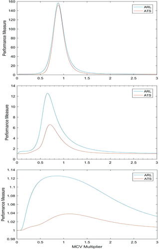
In this section, we will perform additional graphical analysis. To do so, for the chart’s parameters n = (5,15), t = (0.1,1.9), p = 3, for small (0,0.2,0.1), moderate (0.6,0.5,0.6) and large (1.5,2,1.2) mean shifts, we will show how the chart performs when we vary ${\tau }_1$ (in scenario 1) and ${\tau }_2$ (in scenario 2) values from 0.01 to 3, with both their in-control values being 1. This time we choose ${\alpha }_1=0.004$ and ATE = 0.0005. We set ${\mathbf{\mu }}_0=(1,1.5,2)$ and ${\mathbf{\Sigma }}_0=\left[\begin{array}{ccc}1.5\mathrm{ }& 0.6& 0.5\\ 0.6& 1& 0.7\\ 0.5& 0.7& 2\end{array}\right].$

The behavior of the chart when both ${\tau }_1$ and ${\tau }_2$ deviate from their in-control values of 1, is shown in Figures 1 and 2, respectively. The main results from these figures are as follows:

Figure 1. ARL and ATS versus Variability Multiplier (${\tau }_1$) for small, moderate and large (respectively, from top to bottom) mean vector shifts.

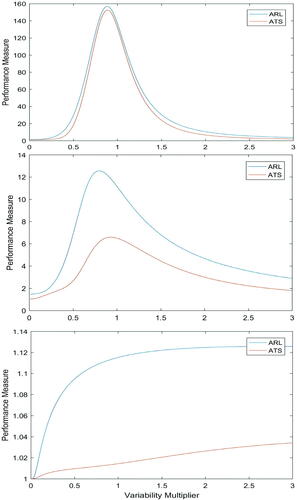
Figure 2. ARL and ATS versus MCV Multiplier (${\tau }_2$) for small, moderate and large (respectively, from top to bottom) mean vector shifts.

• For cases of large mean shifts, in the case of a covariance matrix shift, we have an increasing trend in the chart’s ARL/ATS values up to about the in-control value (${\tau }_1\mathrm{ }\text{or}\mathrm{ }{\tau }_2=1;$ depending on the figure) and a steady bahavior thereafter for large mean shifts. However, in the case of a MCV shift, the chart’s ARL/ATS peaks before, but very close to, the in-control value (${\tau }_2=1$) and goes down if the MCV shifts either upward or downward. The latter trend is valid for the chart with small and moderate mean shifts in both scenarios.

• In both figures, except for the case with a large variability shift in scenario 1, all other plots are right-skewed. Once again, this confirms that the chart detects upward shifts faster than downward shifts and since in scenario 2 the charts are more right-skewed, we can again conclude that it detects MCV upward shifts faster than the covariance matrix upward shifts.

• The ARL and ATS trends are very close in most cases.

6. An illustrative example

For the numerical example, we use a real data set originally used by Hawkins and Maboudou-Tchao (2008), in regards to a healthcare process, for monitoring blood pressure and heart rate, which are in fact the main indicators of heart attack and stroke. For blood pressure and also heart rate, both variance and CV have been used before as a measure of their variation.

The variables of interest are $x_1=$ systolic blood pressure, $x_2=$ diastolic blood pressure, $x_3=$ heart rate and $x_4=$ arterial pressure. Hawkins and Maboudou-Tchao (2008) concluded that the readings for these four characteristics follow the multivariate normal distribution with the below in-control parameter values. $${\mathbf{\mu }}_0=(126.61,77.48,80.95,97.97)\prime \hspace{0.17em}\text{and}\hspace{0.17em}{\mathbf{\Sigma }}_0=\left[\begin{array}{llll}15.04\mathrm{ }& 8.66\mathrm{ }& 10.51& 12.04\\ 8.66\mathrm{ }& 5.83& 5.56& 7.5\\ 10.51\mathrm{ }& \mathrm{ }5.56& 15.17& 8.79\\ 12.04& 7.5& 8.79& 10.57\end{array}\right].$$

Hawkins and Maboudou-Tchao (2008) used two separate control charts for monitoring the mean vector and covariance matrix and they used a single observation in each measurement. If there are no practical restrictions, taking more than one observation, each time a measurement is taken, is always better due to instrumental and environmental issues that exist in most processes; especially for very common biological variables, such as blood pressure and heart rate, which tend to vary constantly. As for the adaptivity of the scheme, it is always better to vary the chart’s parameters, if we can handle the resulting administrative difficulty. Also, using a single chart in the monitoring always makes the procedure easier. Having mentioned these facts, we use our adaptive single chart scheme for a simultaneous monitoring of the mean and variability using the above-mentioned data set.

We assume the below chart’s parameters.

$n_1=5,$ ASS = 7, $n_2=10,$ ASI = 1 hr, $t_2=$ 15min, ATE = 0.005, ${\alpha }_1=$ 0.004 (${\mathit{\text{UCL}}}_1=$ 3.0899). By using Eqs. (6)(6) $$\mathit{\text{UCL}}={\Phi }^{-1}\left[\frac{\sqrt{1-\alpha }+1}{2}\right],$$(6) and (11)–(23), we obtain ${\alpha }_1=$ 0.0065 (${\mathit{\text{UCL}}}_2=$ 2.9425), ${\mathit{\text{UWL}}}_1=$ 1.2082, ${\mathit{\text{UWL}}}_2=$ 1.2957 and $t_1=$ 1.5 hrs.

We start the process monitoring by first shifting the process parameters and taking consecutive samples to test our scheme and observe when it will signal. The shifts we choose are $${\mathbf{\mu }}_1=(126.63,77.38,81,97.88)\prime \hspace{0.17em}\text{and}\hspace{0.17em}{\mathbf{\Sigma }}_1=\left[\begin{array}{cccc}15.44\mathrm{ }& 8.65\mathrm{ }& 10.41& 12.64\\ 8.65\mathrm{ }& 6.83& 5.86& 7.2\\ 10.41\mathrm{ }& \mathrm{ }5.86& 16.07& 8.69\\ 12.64& 7.2& 8.69& 11.07\end{array}\right].$$

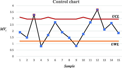
The results are shown in Table 5. For the first sample, we choose the small sample size and long sampling interval (${\Omega }_1$). After taking 5 random observations, we compute the sample mean vector and covariance matrix, and by using Eqs. (3)(3) $$M_i={\Phi }^{-1}\left[H_p(T_i{}^{2\prime })\right]\sim N(0,1),i=1,2,\dots ,$$(3) and (4)(4) $$C{V}_i={\Phi }^{-1}\left[F_{p,n-p,\delta }({\Upsilon }_i)\right]\sim N(0,1),i=1,2,\dots ,$$(4) , we compute the $M_i$ and $C{V}_1$ statistics. Then we combine them using Eq. (5)(5) $$M{V}_i=\mathit{\text{max}}\left\{\left|M_i\right|,\left|C{V}_i\right|\right\}.$$(5) and compute $M{V}_1.$ Since $M{V}_1$ falls in the warning zone ${\mathit{\text{UWL}}}_1<M{V}_1\le {\mathit{\text{UCL}}}_1,$ we should switch to the second set of chart parameters (${\Omega }_2$) for the next sample. This is how the adaptive procedure works. The second column of the table is the sample size used for the current sample, the third column is the cumulative number of observations taken until the current sample, the fourth column is the sampling interval used for the current sample and the fifth column is the cumulative sampling time from the start of process monitoring until the current sample.

Table 5. An illustrative example.

i	$n_i$	$\sum n_i$	$t_i$	$\sum t_i$	$M_i$	$C{V}_i$	$M{V}_i$	${\mathit{\text{UWL}}}_i$	${\mathit{\text{UCL}}}_i$	Status
1	5	5	90	90	1.9003	−0.5333	1.9003	1.2082	3.0899	In-control
2	10	15	15	105	−0.5215	−1.4901	1.4901	1.2057	2.9425	In-control
3	10	25	15	120	3.2695	−0.4504	3.2695	1.2057	2.9425	Out-of-control
4	10	35	15	135	0.8023	0.8023	0.8023	1.2057	2.9425	In-control
5	5	40	90	225	−1.6661	1.6798	1.6798	1.2082	3.0899	In-control
6	10	50	15	240	2.6895	−0.6202	2.6895	1.2057	2.9425	In-control
7	10	60	15	255	1.9056	0.8488	1.9056	1.2057	2.9425	In-control
8	10	70	15	270	0.8585	−1.4680	1.4680	1.2057	2.9425	In-control
9	10	80	15	285	0.5818	−0.8160	0.8160	1.2057	2.9425	In-control
10	5	85	90	375	1.2020	1.7610	1.7610	1.2082	3.0899	In-control
11	10	95	15	390	2.6804	−0.1943	2.6804	1.2057	2.9425	In-control
12	10	105	15	405	−1.2210	3.6799	3.6799	1.2057	2.9425	Out-of-control
13	10	115	15	420	−1.2456	−2.1202	2.1202	1.2057	2.9425	In-control
14	10	125	15	435	−1.8182	2.6203	2.6203	1.2057	2.9425	In-control
15	10	135	15	450	−1.8428	1.3719	1.8428	1.2057	2.9425	In-control

The bold values show the values of the statistic and UCL when the chart signals an out-of-control situation.

As shown in Table 5 and Figure 3, in the first 15 consecutive samplings, the control chart signals at the third and twelfth samples. The chart detects the out-of-control situation after 120 mins have elapsed and 25 observations are taken.

Figure 3. The control chart for the illustrative example.

7. Concluding remarks

This article proposed a new control chart for simultaneously monitoring the multivariate normal process mean and variability. Our proposed scheme is capable of monitoring variability in two forms, i.e., (i) covariance matrix and (ii) MCV. One can choose to monitor either one of them, depending on the type of process at hand. After developing the control chart, adaptive VP features are added to the scheme to make it capable of detecting small and moderate shifts effectively. The ATS and ARL performance measures are computed using a Markov chain model to accurately and quickly measure the chart’s performance. After designing the control scheme, as well as determining how its performance is measured, we conducted numerical analyses, based on two scenarios of variability ((i) covariance matrix and (ii) MCV), for two different number of quality characteristics (p = 2 and 4) and five different sets of chart’s parameters. When either the mean or variability (in any form) shifts from its in-control value, the chart signals, where the larger the shift, the faster the chart signals. However, the MCV chart acts faster. In both scenarios, the chart detects an upward variability shift faster than a downward variability shift. However, the difference is more significant in the first scenario. The performance of the chart in detecting large mean shifts is almost similar for all combinations of the chart’s parameters, different shift combinations and different number of quality characteristics. Another result is that choosing different values of the chart’s parameters will more or less affect the chart’s performance but the trend remains the same. The same goes to using different performance measures (ATS and ARL), as for both measures, the trend remains the same. In both scenarios, as the number of quality characteristics increase, in the ‘no’ or ‘downward’ variation shift, the chart performs worse in most shift situations. On the other hand, in the case of ‘upward’ variation shifts, the chart signals faster if there are more quality characteristics.

For the first scenario (mean and covariance matrix shift), in an upward covariance matrix shift, the more the number of variables where their mean values have shifted, the chart’s performance deteriorates slightly (or there are little differences in the performance). On the contrary to Scenario 1, the previous case is valid for downward MCV shifts.

We also did some additional graphical analyses, based on a set of the chart’s parameters. We presented the findings in two figures (each for one scenario), each containing plots for the small, moderate and large mean shifts when p = 3. These figures confirmed our previous analyses, as well as gave us some new perspectives. They showed that for cases with large mean shifts, in Figure 1 (mean and covariance matrix shift), we have an increasing trend in the chart’s performance measures (ARL and ATS) up to about the in-control value of the covariance matrix and an almost steady behavior thereafter. However, in Figure 2 (mean and MCV shift), the plot peaks ‘before’ but ‘very close’ to the in-control value of the MCV and it goes down for either the upward or downward shift. The latter trend occurs for all other plots in the cases with small and moderate mean shifts and in both scenarios. Finally, we presented an illustrative example based on a real dataset from a healthcare process, which contains four biological quality characteristics, to show how the proposed scheme can be used in practice.

For future extensions, researchers can develop control charts for simultaneous monitoring of the MCV with other process parameters, as this is a new concept. One may also consider measurement errors, autocorrelation and parameter estimation (together or separately) in such schemes.

Acknowledgments

The authors thank the journal’s editorial board and the reviewers for their constructive comments, which have led to significant improvements in the quality of the paper.

References

- Aparisi, F., and C. L. Haro. 2003. A comparison of T2 charts with variable sampling scheme as opposed to MEWMA. International Journal of Production Research 41 (10):2169–82. doi:10.1080/0020754031000138655.
- Aparisi, F., J. Jabaloyes, and A. Carrion. 2001. Generalized variance chart design with adaptive sample sizes. The bivariate case. Communications in Statistics: Simulation and Computation 30 (4):931–48. doi:10.1081/SAC-100107789.
- Calzada, M. E., and S. M. Scariano. 2013. A synthetic control chart for the coefficient of variation. Journal of Statistical Computation and Simulation 83 (5):853–67. doi:10.1080/00949655.2011.639772.
- Castagliola, P., A. Achouri, H. Taleb, G. Celano, and S. Psarakis. 2013a. Monitoring the coefficient of variation using control charts with run rules. Quality Technology & Quantitative Management 10 (1):75–94. doi:10.1080/16843703.2013.11673309.
- Castagliola, P., A. Achouri, H. Taleb, G. Celano, and S. Psarakis. 2013b. Monitoring the coefficient of variation using a variable sampling interval control chart. Quality and Reliability Engineering International 29 (8):1135–49. doi:10.1002/qre.1465.
- Castagliola, P., G. Celano, and S. Psarakis. 2011. Monitoring the coefficient of variation using EWMA charts. Journal of Quality Technology 43 (3):249–65. doi:10.1080/00224065.2011.11917861.
- Chen, Y. K. 2007. Adaptive sampling enhancement of Hotelling’s T2 control charts. European Journal of Operational Research 178 (3):841–57. doi:10.1016/j.ejor.2006.03.001.
- Faraz, A., C. Heuchenne, E. Saniga, and A. Costa. 2014. Double-objective economic statistical design of the VP T2 control chart: Wald’s identity approach. Journal of Statistical Computation and Simulation 84 (10):2123–37. doi:10.1080/00949655.2013.784315.
- Gnanadesikan, M., and S. S. Gupta. 1970. A selection procedure for multivariate normal distributions in terms of the generalized variances. Technometrics 12 (1):103–17. doi:10.1080/00401706.1970.10488638.
- Grigoryan, A., and D. He. 2005. Multivariate double sampling |S| charts for controlling process variability. International Journal of Production Research 43 (4):715–30. doi:10.1080/00207540410001716525.
- Hawkins, D. M., and E. M. Maboudou-Tchao. 2008. Multivariate exponentially weighted moving covariance matrix. Technometrics 50 (2):155–66. doi:10.1198/004017008000000163.
- Hong, E. P., C. W. Kang, J. W. Baek, and H. W. Kang. 2008. Development of CV control chart using EWMA technique. Journal of the Society of Korea Industrial and Systems Engineering 31 (4):114–20.
- Kang, C. W., M. S. Lee, Y. J. Seong, and D. M. Hawkins. 2007. A control chart for the coefficient of variation. Journal of Quality Technology 39 (2):151–8. doi:10.1080/00224065.2007.11917682.
- Khaw, K. W., M. Khoo, P. Castagliola, and M. A. Rahim. 2018. New adaptive control charts for monitoring the multivariate coefficient of variation. Computers & Industrial Engineering 126:595–610. doi:10.1016/j.cie.2018.10.016.
- Khaw, K. W., M. Khoo, W. C. Yeong, and Z. Wu. 2017. Monitoring the coefficient of variation using a variable sample size and sampling interval control chart. Communications in Statistics - Simulation and Computation 46 (7):5772–94. doi:10.1080/03610918.2016.1177074.
- Khoo, M. B. C. 2005. A new bivariate control chart to monitor the multivariate process mean and variance simultaneously. Quality Engineering 17 (1):109–18. doi:10.1081/QEN-200028718.
- Lee, M. H., and M. B. C. Khoo. 2015. Multivariate synthetic |S| control chart with variable sampling interval. Communications in Statistics - Simulation and Computation 44 (4):924–42. doi:10.1080/03610918.2013.796980.
- Matrix, C., M. R. Reynolds, and G.-Y. Cho. 2006. Multivariate control charts for monitoring the mean vector and covariance matrix. Journal of Quality Technology 38 (3):230–53. doi:10.1080/00224065.2006.11918612.
- Nguyen, Q. T., K. P. Tran, H. L. Heuchenne, T. H. Nguyen, and H. D. Nguyen. 2019. Variable sampling interval Shewhart control charts for monitoring the multivariate coefficient of variation. Applied Stochastic Models in Business and Industry 35 (5):1253–68. doi:10.1002/asmb.2472.
- Noor-ul-Amin, M., S. Tariq, and M. Hanif. 2019. Control charts for simultaneously monitoring of process mean and coefficient of variation with and without auxiliary information. Quality and Reliability Engineering International 35 (8):2639–56. doi:10.1002/qre.2546.
- Reed, G. F., F. Lynn, and B. D. Meade. 2002. Use of coefficient of variation in assessing variability of quantitative assays. Clinical and Diagnostic Laboratory Immunology 9 (6):1235–9.
- Reynolds, M. R., Jr., and G. Y. Cho. 2006. Multivariate control charts for monitoring the mean vector and covariance matrix. Journal of Quality Technology 38 (3):230–53.
- Reynolds, M. R., Jr., and G. Y. Cho. 2011. Multivariate control charts for monitoring the mean vector and covariance matrix with variable sampling intervals. Sequential Analysis 30 (1):1–40. doi:10.1080/07474946.2010.520627.
- Reynolds, M. R., Jr., and K. Kim. 2007. Multivariate control charts for monitoring the process mean and variability using sequential sampling. Sequential Analysis 26 (3):283–315. doi:10.1080/07474940701404898.
- Sabahno, H., A. Amiri, and P. Castagliola. 2018a. Evaluating the effect of measurement errors on the variable sampling intervals Hotelling T2 control charts. Quality and Reliability Engineering International 34 (8):1785–99. doi:10.1002/qre.2370.
- Sabahno, H., A. Amiri, and P. Castagliola. 2018b. Optimal performance of the variable sample sizes Hotelling’s T2 control chart in the presence of measurement errors. Quality Technology & Quantitative Management 16 (5):588–612. doi:10.1080/16843703.2018.1490474.
- Sabahno, H., A. Amiri, and P. Castagliola. 2021. A new adaptive control chart for the simultaneous monitoring of the mean and variability of multivariate normal processes. Computers & Industrial Engineering 151:106524. doi:10.1016/j.cie.2020.106524.
- Sabahno, H., P. Castagliola, and A. Amiri. 2020a. A variable parameters multivariate control chart for simultaneous monitoring of the process mean and variability with measurement errors. Quality and Reliability Engineering International 36 (4):1161–96. doi:10.1002/qre.2621.
- Sabahno, H., P. Castagliola, and A. Amiri. 2020b. An adaptive variable-parameters scheme for the simultaneous monitoring of the mean and variability of an autocorrelated multivariate normal process. Journal of Statistical Computation and Simulation 90 (8):1430–65. doi:10.1080/00949655.2020.1730373.
- Seif, A., A. Faraz, E. Saniga, and C. Heuchenne. 2016. A statistically adaptive sampling policy to the Hotelling’s T2 control chart: Markov Chain approach. Communications in Statistics - Theory and Methods 45 (13):3919. doi:10.1080/03610926.2014.911910.
- Voinov, V. G., and M. S. Nikulin. 1996. Unbiased estimators and their applications, multivariate case. Vol. 2. Kluwer: Dordrecht.
- Wang, K., A. B. Yeh, and B. Li. 2014. Simultaneous monitoring of process mean vector and covariance matrix via penalized likelihood estimation. Computational Statistics & Data Analysis 78 (1):206–17. doi:10.1016/j.csda.2014.04.017.
- Wijsman, R. A. 1957. Random orthogonal transformations and their use in some classical distribution problems in multivariate analysis. The Annals of Mathematical Statistics 28 (2):415–23. doi:10.1214/aoms/1177706969.
- Yeong, W. C., M. Khoo, W. L. Teoh, and P. Castagliola. 2016. A control chart for the multivariate coefficient of variation. Quality and Reliability Engineering International 32 (3):1213–25. doi:10.1002/qre.1828.
- Zhang, G., and S. I. Chang. 2008. Multivariate EWMA control charts using individual observations for process mean and variance monitoring and diagnosis. International Journal of Production Research 46 (24):6855–81. doi:10.1080/00207540701197028.
- Zhang, J., Z. Li, and Z. Wang. 2010. A multivariate control chart for simultaneously monitoring process mean and variability. Computational Statistics & Data Analysis 54 (10):2244–52. doi:10.1016/j.csda.2010.03.027.
- Zhang, J., Z. Li, B. Chen, and Z. Wang. 2014. A new exponentially weighted moving average control chart for monitoring the coefficient of variation. Computers & Industrial Engineering 78:205–12. doi:10.1016/j.cie.2014.09.027.