Alternative bootstrap confidence regions for multiple correspondence analysis

Abstract

A new approach for constructing elliptical bootstrap confidence regions for Multiple Correspondence Analysis is proposed, where the difference in method follows directly from the adoption of a different objective criterion to previous approaches. This includes a new correction for the well-known problems caused by the diagonal of the Burt matrix. Simulation experiments show that the method performs reasonably well in many cases, with exceptions being noted. Simulated data sets with known structure are also used to illustrate cases where the proposed method produces results in line with what would be expected, but some alternatives do not.

Keywords:

• Bootstrapping
• Burt matrix
• Confidence region
• Correspondence analysis
• Stability

1. Introduction

Correspondence Analysis (CA) is a family of methods for the graphical display of bivariate or multivariate categorical data in low-dimensional space, analogous to the graphical use of Principal Component Analysis (PCA) for continuous data. Simple Correspondence Analysis (SCA) deals with the bivariate case of a contingency table of counts while Multiple Correspondence Analysis (MCA) applies the same algebra to different codings of the multivariate case.

The most usual output is a scatter plot giving the best two-dimensional representation of the data, where each plotted point represents one category of one of the categorical variables. Categories which co-occur will tend to plot close to each other, so that CA, again like PCA, gives a convenient graphical representation of the correlation structure of the data.

However, this purely algorithmic and geometrical approach ignores random variation in the data and can easily result in the over-interpretation of what may be ‘noise’. Previous work has considered the creation of confidence circles, ellipses or convex hulls for these category points in both SCA and MCA using various different assumptions and objectives and using both algebraic and computational approaches (Greenacre 1984; Lebart, Morineau, and Warwick 1984; Ringrose 1992; Markus, 1994a, 1994b; Michailidis and de Leeuw 1998; Lebart 2006; Lê, Josse, and Husson 2008; Beh 2010; Ringrose 2012; D'Ambra and Crisci 2014; Beh and Lombardo 2015; Iacobucci and Grisaffe 2018; Corral-De-Witt et al. 2019; González-Serrano et al. 2020; D’Ambra, Amenta, and Beh 2021; Alzahrani, Beh, and Stojanovski 2023; D’Ambra and Amenta 2023).

Confidence regions for SCA started with circles (Lebart, Morineau, and Warwick 1984) and later ellipses (Beh 2010; Beh and Lombardo 2015) based on the ${\chi }^2$ test, so that these can be thought of as graphical illustrations of tests for independence, rather than confidence regions for the projected points per se, while the first uses of resampling to produce confidence regions for SCA (Greenacre 1984; Ringrose 1992) ignored sampling variation in the axes as well as the correlation between axes and points. Subsequent bootstrap approaches to confidence regions for SCA and MCA (Markus, 1994a, 1994b; Michailidis and de Leeuw 1998; Lebart 2006; Ringrose 2012; Corral-De-Witt et al. 2019; González-Serrano et al. 2020) have addressed these problems, but all except (Ringrose 2012) have considered variation in the sample points projected onto the sample axes, which means that they are implicitly confidence regions for the population points projected onto the population axes, as explained in Sec. 3.

The present work proposes new confidence ellipses for the MCA case, building on the work in Ringrose (2012, 1996), and uses a different approach to those used for previous MCA confidence ellipses, which are implicitly defined such that a 95% confidence ellipse will contain the unknown population point projected onto the unknown population axes in 95% of samples, as explained in Sec. 3. The main motivation for the new approach is that it allows the construction of confidence regions such that a 95% confidence ellipse will instead contain the unknown population point projected onto the observed sample axes in 95% of samples, which the author regards as the most natural extension of the usual definition of a confidence interval to the case of multivariate projection methods. In order to achieve this, the key methodological distinction is that this method explicitly deals with sampling variation in the difference between sample and population points when both are projected onto the observed sample axes, rather than sampling variation in just the sample points projected onto the observed sample axes. The reasoning behind this is given in detail in Ringrose (2012, 1996) and summarized in Sec. 4. These new ellipses also propose a new way to deal with the well-known problem of the distorting effect of the diagonal of the Burt matrix in MCA.

Hence the proposed method can be thought of as a different definition of what we require from MCA confidence regions, thus leading to a different procedure to construct them. However, there are some situations where it can be agreed what the results should be, for example with completely random data, where we would expect confidence regions to be large and substantially overlapping each other. It is shown in Sec. 5 that in this case the widely used Factominer package can produce ellipses that are misleadingly small, whereas the proposed method with the correction for the diagonal of the Burt matrix produces ellipses that conform to the above expectation.

Section 2 summarizes and defines notation for simple and multiple CA. Section 3 summarizes the existing methods to construct confidence regions for SCA and MCA, then Sec. 4 describes and justifies the proposed new method, emphasizing the differences in approach. Section 5 compares results from the proposed method to those from other methods, using illustrative simulated data, in cases where comparisons can reasonably be made. Section 6 describes a simulation study to assess the performance of the new method, Sec. 7 gives an example application and Sec. 8 summarizes and discusses the conclusions.

In the following the convention used is that in most cases capitals (W) are matrices, bold face letters (w) are column vectors and small case letters (w) are scalars. The i, j-th element of W is w_ij and the j-th element of w is w_j. A column vector of 1s is denoted 1. The superscript ${()}^T$ denotes the transpose. In some cases the j-th column of W is ${\mathit{w}}_j$ or the j-th row of W is ${\mathit{w}}_j^T,$ but never both, to avoid notational confusion. For any sample quantity such as W, the corresponding population quantity is denoted $W^{‡}$ and the bootstrap quantity is denoted $W^{\star }.$

2. Correspondence analysis

The notation and terminology used here will largely follow that in Greenacre (1984).

2.1. Simple correspondence analysis

This works with any matrix of non-negative values, but is usually applied to bivariate categorical data where two categorical variables with I and J categories form a contingency table of counts X_CT. This table is then divided by the sum n of its elements, usually the number of individuals who have been cross-classified, to give an I × J matrix X of non-negative values x_ij which sum to 1. Then let $\mathit{r}=X\mathbf{1}$ and $\mathit{c}=X^T\mathbf{1}$ be the vectors of row and column sums of X respectively, with $D_{\mathit{r}}=\text{diag}(\mathit{r})$ and $D_{\mathit{c}}=\text{diag}(\mathit{c}).$

Then the i-th row profile ${\mathit{r}}_i^T$ is the i-th row of X divided by its sum, and is the i-th row of the row profile matrix $R=D_{\mathit{r}}^{-1}X.$ Column profiles are defined analogously by dividing columns of X by their sum, giving ${\mathit{c}}_j^T$ the j-th row of the column profile matrix $C=D_{\mathit{c}}^{-1}{X}^T.$ Then SCA finds a low-dimensional representation of the rows of R with point ‘masses’ in r and inverse dimension weights in c, and simultanaeously a low-dimensional representation of the rows of C with point ‘masses’ in c and inverse dimension weights in r.

All results are derived from the Singular Value Decomposition (SVD) of the weighted, centered data matrix Z, giving (1) $$Z=D_{\mathit{r}}^{-\frac{1}{2}}(X-\mathit{r}{\mathit{c}}^T)D_{\mathit{c}}^{-\frac{1}{2}}=U{D}_{\mathit{\mu }}{V}^T$$(1) where $D_{\mathit{\mu }}=\text{diag}(\mathit{\mu })$ contains the ordered singular values ${\mu }_1\ge \dots \ge {\mu }_{r_{\mathrm{\text{max}}}}\ge 0$ and $r_{\mathrm{\text{max}}}=\mathrm{\text{min}}(I,J)-1$ is the (maximum) rank of Z. The squared singular values ${\lambda }_i={\mu }_i^2$ are the eigenvalues of Z^TZ and represent the total ‘inertia’ of each axis, analogous to the variance of each axis in PCA. The columns of V are the right singular vectors of Z, the eigenvectors of Z^TZ, forming an orthonormal basis for the rows of Z (i.e. $V^{T}V=I$). The columns of U are the left singular vectors of Z, the eigenvectors of ZZ^T, forming an orthonormal basis for the columns of Z (i.e. $U^{T}U=I$).

The centered row profiles in $R-\mathbf{1}{\mathit{c}}^T$ are projected onto axes $D_{\mathit{c}}^{\frac{1}{2}}V$ with dimension weights in $D_{\mathit{c}}^{-1}$ giving a matrix of row coordinates F, which can be expressed in several different ways as (2) $$F=(R-\mathbf{1}{\mathit{c}}^T)D_{\mathit{c}}^{-1}\left(D_{\mathit{c}}^{\frac{1}{2}}V\right)=R{D}_{\mathit{c}}^{-\frac{1}{2}}V=D_{\mathit{r}}^{-\frac{1}{2}}U{D}_{\mathit{\mu }}={\mathit{\text{RGD}}}_{\mathit{\mu }}^{-1}$$(2) with the coordinates for the i-th row category in ${\mathit{f}}_i^T,$ the i-th row of F.

Similarly the column profiles in $C-\mathbf{1}{\mathit{r}}^T$ are projected onto axes $D_{\mathit{r}}^{\frac{1}{2}}U$ with dimension weights in $D_{\mathit{r}}^{-1}.$ Hence the coordinates for the j-th column category are in ${\mathit{g}}_j^T,$ the j-th row of (3) $$G=(C-\mathbf{1}{\mathit{r}}^T)D_{\mathit{r}}^{-1}\left(D_{\mathit{r}}^{\frac{1}{2}}U\right)=C{D}_{\mathit{r}}^{-\frac{1}{2}}U=D_{\mathit{c}}^{-\frac{1}{2}}V{D}_{\mathit{\mu }}={\mathit{\text{CFD}}}_{\mathit{\mu }}^{-1}$$(3)

Both (2)(2) $$F=(R-\mathbf{1}{\mathit{c}}^T)D_{\mathit{c}}^{-1}\left(D_{\mathit{c}}^{\frac{1}{2}}V\right)=R{D}_{\mathit{c}}^{-\frac{1}{2}}V=D_{\mathit{r}}^{-\frac{1}{2}}U{D}_{\mathit{\mu }}={\mathit{\text{RGD}}}_{\mathit{\mu }}^{-1}$$(2) and (3)(3) $$G=(C-\mathbf{1}{\mathit{r}}^T)D_{\mathit{r}}^{-1}\left(D_{\mathit{r}}^{\frac{1}{2}}U\right)=C{D}_{\mathit{r}}^{-\frac{1}{2}}U=D_{\mathit{c}}^{-\frac{1}{2}}V{D}_{\mathit{\mu }}={\mathit{\text{CFD}}}_{\mathit{\mu }}^{-1}$$(3) are in ‘principal coordinates’ where the axes are weighted by their singular values, the alternative being ‘standard coordinates’ where these weightings are omitted, giving $F_{\mathit{\text{std}}}=D_{\mathit{r}}^{-\frac{1}{2}}U$ and $G_{\mathit{\text{std}}}=D_{\mathit{c}}^{-\frac{1}{2}}V.$

Most applications of SCA then involve plotting and interpretation of the first two dimensions of the data, given by the first two columns of F and G in ‘French-style’ plots or by the first two columns of F and G_std or G and F_std for biplot-style plots. For further details see Greenacre (1984) and Ringrose (2012).

2.2. Multiple correspondence analysis

This covers the case of multivariate categorical data, and uses the same algebra as in Sec. 2.1 but applied to different codings of the data. It is described more fully in Greenacre (1984) and Greenacre and Blasius (2006) and also in Gifi (1990) under the name Homogeneity Analysis and in Nishisato (1994) under the name Dual Scaling. The similarities and differences between the French school (MCA) and the Dutch school (Homogeneity Analysis) are described in Di Franco (2016).

In SCA the matrix X is usually the two-way contingency table X_CT divided by its sum n, but for the p-way case there are two main alternatives. Consider an n individuals by p variables matrix X_np where the i-th row contains the category names/numbers to which the i-th individual belongs and where the k-th variable has J_k distinct categories. This can then be converted into the indicator matrix X_Ind where the k-th column of X_np becomes J_k columns in X_Ind, with the i-th row containing one in the column corresponding to the category to which the i-th individual belongs, and zeros elsewhere. Hence each row contains exactly one value of one in each set of J_k columns and all of the row sums are p. Hence X_Ind is n by $J={\sum }_{k=1}^p{J}_k$ and the elements sum to np.

The Burt matrix is constructed as $X_{\mathit{\text{Burt}}}=X_{\mathit{\text{Ind}}}^T{X}_{\mathit{\text{Ind}}}$ and so is a block diagonal J × J matrix with the k₁, k₂-th block containing the two-way contingency table cross-classifying the k₁-th and k₂-th variables. The diagonal blocks contain the variables cross-classified with themselves, and so are all diagonal and uninformative. When p = 2 the top right block of the Burt matrix is X_CT and the bottom left block is $X_{\mathit{\text{CT}}}^T.$

The indicator matrix and the Burt matrix can each be divided by their respective sums and the resulting matrix X be analyzed using exactly the same algebra as SCA in Sec. 2.1. The results are very similar but not identical to each other and also, in the p = 2 case, not identical to the SCA results. The connections and possible corrections that can be applied are explained in Greenacre and Blasius (2006, Chapter 2), but details will be deferred until Sec. 4.3 when they become relevant. Note that, since all the information used is contained in the Burt matrix, MCA is really multiply bivariate rather than truly multivariate.

It can be argued that MCA is a generalization of SCA, or that it is a different method to SCA that happens to share the same algebra. The position taken here is closer to the former view, so that if the results for MCA with p = 2 are similar to those for SCA then this is regarded as a good thing, but it is acknowledged that not all practitioners will agree.

3. Confidence regions for correspondence analysis

In both the SCA and MCA cases different types of confidence region (CR) have been proposed based on different philosophies and objectives. There are different views of what a 95% confidence region means, i.e. which event is expected to happen in approximately 95% of samples. Hence comparisons between methods are often comparisons between their aims rather than between their performances, because a method’s performance can usually only be compared to that method’s aims. A partial exception to this is that in some cases we can say clearly what we would expect the graphical results should look like, as in Sec. 5.

Many methods have been proposed for SCA CR starting with simple circles in Lebart, Morineau, and Warwick (1984) which were developed into improved ellipses in Beh (2010) and Beh and Lombardo (2015). These are reviewed in Ringrose (2012), and the following description of the differing approaches is a shortened version of that in Ringrose (2012), with the addition of more recent references.

The earliest resampling approaches Greenacre (1984) and Ringrose (1992) used bootstrap replications of the data but simply projected the bootstrap row and column profiles onto the existing sample axes as supplementary points and used convex hull peeling to produce ad hoc confidence regions, although ellipses can also be constructed. However, this approach, referred to in Lebart (2006, 2007a, 2007b) as the partial bootstrap, ignores the variability in the sample axes and the correlation between the sample axes and the sample row and column profiles, so that the regions tend to be too small.

In the present paper, as in Ringrose (2012), the aim is to put a CR around a plotted sample point such that a 95% CR should contain the population point projected onto these same axes in 95% of samples. In the SCA case this entails a CR around the j-th projected sample column point ${\mathit{g}}_j^T={\mathit{c}}_j^T{D}_{\mathit{r}}^{-\frac{1}{2}}U,$ with the j-th population point ${\mathit{c}}_j^{‡T}$ then being projected as a supplementary point onto the same sample axes $D_{\mathit{r}}^{-\frac{1}{2}}U$ (and similarly for row points or other confidence levels). A similar approach can be applied to the MCA case, as described in Sec. 4. A CR of this type must hence be based on the variability in ${({\mathit{c}}_j-{\mathit{c}}_j^{‡})}^T{D}_{\mathit{r}}^{-\frac{1}{2}}U,$ the difference between the sample point and the population point when both are projected onto the sample axes.

However, previous approaches are based on the variability in the sample coordinates ${\mathit{c}}_j^T{D}_{\mathit{r}}^{-\frac{1}{2}}U,$ i.e. in the sample point projected onto the sample axes. Hence if viewed as CRs, a 95% CR of this type around a plotted sample point would implicitly be required to contain the population coordinates ${\mathit{g}}_j^{‡T}={\mathit{c}}_j^{‡T}{D}_{\mathit{r}}^{‡-\frac{1}{2}}{U}^{‡},$ i.e. the population point projected onto the population axes, in 95% of samples.

The view taken here, as in Ringrose (2012, 1996, 1994), is that comparing points projected onto different axes, i.e. sample and population axes in this case, is rarely useful, particularly since population axes are usually of little interest, especially when singular values are close so that population and sample axes may be quite different.

The CR for MCA proposed in Markus (1994a, 1994b) and Michailidis and de Leeuw (1998) and the full bootstrap method in Lebart (2006) are of the second type above, as are those for SCA proposed in Iacobucci and Grisaffe (2018). Those proposed in Corral-De-Witt et al. (2019) and González-Serrano et al. (2020) are slightly different in that they use kernel density estimation, but are again of this second type. Hence these all assess the stability of the graphical display and can be thought of as sensitivity analysis or internal validation, rather than being CR of the type proposed here.

The original CR for SCA in Lebart, Morineau, and Warwick (1984), Beh (2010), Beh and Lombardo (2015), and Alzahrani, Beh, and Stojanovski (2023) are also of the second type above and are derived assuming a null hypothesis of independence of row and column categories. These can hence be thought of as a graphical illustration of the decomposition of the ${\chi }^2$ test for a contingency table, rather than being CR of the type proposed here. The CR for multiple non-symmetric CA for the p = 3 case in D'Ambra and Crisci (2014), those for a version of CA based on cumulative frequencies for ordinal data in D’Ambra, Amenta, and Beh (2021), and those for three-way CA with ordinal data in D’Ambra and Amenta (2023), are also based on those in Beh (2010).

The R package Factominer Lê, Josse, and Husson (2008) does not contain a reference or description of the exact methods it uses to produce CR for SCA and MCA, but it seems to be similar to the partial bootstrap method in Lebart (2006), where resampled data points are projected onto the sample axes and ellipses are then constructed based on the eigenvalues of a PCA of these coordinates. Some simple empirical comparisons will be made in Sec. 5.

4. New confidence regions for multiple correspondence analysis

The confidence regions proposed here are of the first type described in Sec. 3, following the approach described in Ringrose (2012, 1996, 1994). They are hence based on the sampling variation of the difference between sample and population points when both are projected onto the sample axes, allowing for variation in both the points and the axes and the correlation between them. Hence the nominal coverage percentage is the probability of drawing a sample from the population which is such that the constructed confidence ellipse contains the population point when the latter is projected onto the samples axes as a supplementary point.

MCA can be applied to the indicator matrix X_Ind or the Burt matrix X_Burt, but for reasons which will become clear MCA is here only applied to the Burt matrix. This is symmetrical, so that there are both J row points and J column points, each point representing a single category from a single variable, and all row results and column results are the same. In all the descriptions below the J column points are taken as the data points which will be plotted and for which CR are sought, as this seems most natural. Hence in the descriptions below X in Eq. (1)(1) $$Z=D_{\mathit{r}}^{-\frac{1}{2}}(X-\mathit{r}{\mathit{c}}^T)D_{\mathit{c}}^{-\frac{1}{2}}=U{D}_{\mathit{\mu }}{V}^T$$(1) is X_Burt divided by its sum and the formulae for coordinates and axes come from Eq. (3)(3) $$G=(C-\mathbf{1}{\mathit{r}}^T)D_{\mathit{r}}^{-1}\left(D_{\mathit{r}}^{\frac{1}{2}}U\right)=C{D}_{\mathit{r}}^{-\frac{1}{2}}U=D_{\mathit{c}}^{-\frac{1}{2}}V{D}_{\mathit{\mu }}={\mathit{\text{CFD}}}_{\mathit{\mu }}^{-1}$$(3) .

4.1. Confidence ellipses

We require a CR around the j-th variable category point ${\mathit{c}}_j^T$ which will contain the population point ${\mathit{c}}_j^{‡T}$ with the chosen nominal coverage probability, projecting both onto the sample axes $D_{\mathit{r}}^{-\frac{1}{2}}U.$ Hence to construct a CR for the first and second axes we require the 2 × 2 variance matrices $\text{Var}({\mathit{d}}_j)={\Sigma }_{d_j}$ where (4) $${\mathit{d}}_j^T=({\mathit{c}}_j^T-{\mathit{c}}_j^{‡T})D_{\mathit{r}}^{-\frac{1}{2}}[{\mathit{u}}_1 {\mathit{u}}_2]j=1\dots J$$(4) This should have approximately zero mean and its variance matrix accounts for sampling variation in both the sample axes and the sample points, and the correlation between them.

If ${\Sigma }_{d_j}$ is estimated by ${\widehat{\Sigma }}_{d_j}$ then a confidence ellipse can be drawn using (5) $${\mathit{d}}_j^T{\widehat{\Sigma }}_{d_j}^{-1}{\mathit{d}}_j\le {\chi }_{\mathit{\text{crit}}}$$(5) If ${\mathit{d}}_j$ can be assumed to be approximately (bivariate) normal then the critical value χ_crit is taken from ${\chi }_2^2$ and hence will be 5.991 for a 95% ellipse.

As in Markus (1994a, 1994b), Michailidis and de Leeuw (1998), and Ringrose (2012, 1996, 1994) the covariance matrices for Eq. (4)(4) $${\mathit{d}}_j^T=({\mathit{c}}_j^T-{\mathit{c}}_j^{‡T})D_{\mathit{r}}^{-\frac{1}{2}}[{\mathit{u}}_1 {\mathit{u}}_2]j=1\dots J$$(4) are estimated using bootstrapping, and here the critical values for Eq. (5)(5) $${\mathit{d}}_j^T{\widehat{\Sigma }}_{d_j}^{-1}{\mathit{d}}_j\le {\chi }_{\mathit{\text{crit}}}$$(5) will also be estimated using bootstrapping.

4.2. Bootstrap algorithm

The variance matrices ${\Sigma }_{d_j}$ are estimated by non-parametric boostrapping, i.e. sampling with replacement from the rows of X_np to generate a large number b of resampled data matrices $X_{\mathit{\text{np}}}^{\star }.$ Then MCA is applied to the Burt matrix of each of these and ${\widehat{\Sigma }}_{d_j}$ calculated using the b bootstrap replicates of (6) $${\mathit{d}}_j^{\star T}=({\mathit{c}}_j^{\star T}-{\mathit{c}}_j^T)D_{\mathit{r}}^{\star -\frac{1}{2}}[{\mathit{u}}_{(1)}^{\star } {\mathit{u}}_{(2)}^{\star }]j=1\dots J$$(6) Note that ${\mathit{u}}_{(1)}^{\star },{\mathit{u}}_{(2)}^{\star }$ are not necessarily the first two columns of $U^{\star },$ but are instead the columns of $U^{\star }$ which most closely match ${\mathit{u}}_1,{\mathit{u}}_2,$ the axes being used in the plot.

This important difference is because axes can reorder as well as rotate and reflect from sample to sample, i.e. the axis with the largest singular value in the population will not necessarily have the largest singular value in any given sample. If this is not accounted for then the variances will be estimated using some entirely different axes due to reordering, instead of being based on the sample to sample rotations of the equivalent axes. This will inflate the variances with spurious variation. Hence here the bootstrap axes are matched as closely as possible to the sample axes using the Hungarian algorithm, and are also reflected to match the sample axes when needed. The CR in Markus (1994a, 1994b) and Iacobucci and Grisaffe (2018) also recognized this problem but instead used Procrustes rotations of the bootstrap coordinates relative to the sample coordinates, which tends to over-correct. This is explained in more detail in Ringrose (2012, Sec. 3.3).

As in Ringrose (2012, 1996, 1994), and mentioned in Milan and Whittaker (1995) and Lebart (2007a, 2007b), the axes are hence ‘rearranged’ to remove spurious variation caused by reordering and reflection of axes, but not the genuine variation caused by rotation of the axes. This is referred to in Lebart (2007a, 2007b) as total bootstrap type 2, while the Procrustes rotation approach is total bootstrap type 3.

In SCA and MCA the use of the SVD means that row and column axes must have the same reorderings and reflections. The sample and bootstrap axes are taken to be the columns of U, V and $U^{\star },V^{\star }$ respectively, and the Hungarian algorithm implemented in the R package lpSolve routine lp.assign Berkelaar (2023) is used to find the ‘allocation’ of bootstrap axes to sample axes to maximize (7) $$\sum _{k=1}^{r_{\mathrm{\text{max}}}}|{\mathit{u}}_k^T{\mathit{u}}_{(k)}^{\star }+{\mathit{v}}_k^T{\mathit{v}}_{(k)}^{\star }|\text{\hspace{0.5em}where\hspace{0.5em}}{\mathit{v}}_{(k)}^{\star }={\mathit{v}}_j^{\star },{\mathit{u}}_{(k)}^{\star }={\mathit{u}}_j^{\star }\text{\hspace{0.5em}for\hspace{0.5em}distinct\hspace{0.5em}}j$$(7) which summarizes the overall closeness of sample to rearranged bootstrap axes. Note that the singular values are not used in this allocation, so that some over-correction may still occur. An alternative would be the method described in Sharpe and Fieller (2016) in the context of functional PCA, of only considering reorderings of eigenvectors that are close in the original ordering, hence to some extent using the information provided by the singular values.

This axis rearrangement is the reason why only the Burt matrix is considered here. In the Burt case the elements of the vectors ${\mathit{u}}_k,{\mathit{u}}_{(k)}^{\star },{\mathit{v}}_k,{\mathit{v}}_{(k)}^{\star }$ correspond to the rows of X, which are the J variable categories and are the same in every bootstrap replicate, provided care is taken when a category does not appear in some bootstrap replicates. When X is based on the indicator matrix the rows will instead be the resampled individuals and hence different in every replicate, so that the allocation/matching in Eq. (7)(7) $$\sum _{k=1}^{r_{\mathrm{\text{max}}}}|{\mathit{u}}_k^T{\mathit{u}}_{(k)}^{\star }+{\mathit{v}}_k^T{\mathit{v}}_{(k)}^{\star }|\text{\hspace{0.5em}where\hspace{0.5em}}{\mathit{v}}_{(k)}^{\star }={\mathit{v}}_j^{\star },{\mathit{u}}_{(k)}^{\star }={\mathit{u}}_j^{\star }\text{\hspace{0.5em}for\hspace{0.5em}distinct\hspace{0.5em}}j$$(7) would not make sense.

4.3. The problem of the Burt matrix

It is well-known that in MCA the results are distorted by the diagonal elements of the Burt matrix, and these are often corrected by adjusting the raw singular values μ_i and hence the principal coordinates. The usual correction for the Burt diagonal Greenacre and Blasius (2006, 67–68) is to ignore all singular values less than $1/p$ and for the others to use adjusted singular values $${\mu }_k^{\mathit{\text{adj}}}=\frac{p}{p-1}\left({\mu }_k-\frac{1}{p}\right) {\mu }_k\ge \frac{1}{p}$$

These are used to calculate the adjusted inertias ${\lambda }_k^{\mathit{\text{adj}}}={({\mu }_k^{\mathit{\text{adj}}})}^2$ and hence also adjusted coordinates, so that the j-th column point becomes (8) $${\mathit{g}}_j^{\mathit{\text{adj}}}={\mathit{g}}_j\times \frac{p}{p-1}\left({\mu }_k-\frac{1}{p}\right)\times \frac{1}{{\mu }_k} j=1\dots J,{\mu }_k\ge \frac{1}{p}$$(8)

However, even when these standard corrections are used, if bootstrapping is applied in the usual way then the estimated variances may be too small because the diagonal elements of the standardized Burt matrix are the same in every bootstrap replicate, thus underestimating the true variation in the data. Hence a new method is proposed here to correct for this when bootstrapping.

If a variable category appears k times then that row (or column) in the Burt matrix consists of p blocks each of which sum to k, so its row (and column) sum is kp. The diagonal element is the variable category cross-classified with itself, so it is just k. Therefore when the row (or column) profile matrix is calculated the diagonal elements of the Burt matrix are always all $1/p$ while the elements for the categories in the off-diagonal blocks sum to $1/p$ in each block. Hence in the proposed method when the projected difference between the sample and resample column profile matrices is calculated this is artificially small because the diagonals of the two matrices are always the same, no matter how different the off-diagonal elements are. Hence it is clear that for the proposed method this feature of the Burt matrix will cause the variances to be underestimated. It is less obvious how it affects other proposed methods, but the fact that one part of the Burt matrix is the same in every bootstrap replicate suggests that a similar problem occurs.

The new method proposed here to correct for the diagonal elements of the Burt matrix when calculating variances does so by re-expressing the coordinates of the column points purely in terms of the off-diagonal elements of the Burt matrix which vary from sample to sample, without using the constant and hence uninteresting diagonal elements.

First calculate the Burt principal coordinates with the diagonal elements of the profile matrix ignored or set to zero and denote these ${\mathit{g}}_j^{\mathit{\text{nondiag}}}.$ A key point is that because the diagonal elements of the Burt matrix are always the same, the difference between C and $C^{\star }$ in these elements will always be zero, so that when calculating Eq. (6)(6) $${\mathit{d}}_j^{\star T}=({\mathit{c}}_j^{\star T}-{\mathit{c}}_j^T)D_{\mathit{r}}^{\star -\frac{1}{2}}[{\mathit{u}}_{(1)}^{\star } {\mathit{u}}_{(2)}^{\star }]j=1\dots J$$(6) in effect it is already ${\mathit{g}}_j^{\mathit{\text{nondiag}}}$ which is being calculated.

It is easy to verify that the usual Burt principal coordinates can be re-expressed using the singular values as (9) $${\mathit{g}}_j=\frac{{\mu }_k}{\left({\mu }_k-\frac{1}{p}\right)}\times {\mathit{g}}_j^{\mathit{\text{nondiag}}}$$(9)

When using the usual adjusted/corrected coordinates and inertias Eqs. (8)(8) $${\mathit{g}}_j^{\mathit{\text{adj}}}={\mathit{g}}_j\times \frac{p}{p-1}\left({\mu }_k-\frac{1}{p}\right)\times \frac{1}{{\mu }_k} j=1\dots J,{\mu }_k\ge \frac{1}{p}$$(8) and (9)(9) $${\mathit{g}}_j=\frac{{\mu }_k}{\left({\mu }_k-\frac{1}{p}\right)}\times {\mathit{g}}_j^{\mathit{\text{nondiag}}}$$(9) will both be applied, thus producing a simple correction factor of $p/(p-1).$ Hence the bootstrap algorithm is applied as usual and ${\mathit{d}}_j$ in Eq. (6)(6) $${\mathit{d}}_j^{\star T}=({\mathit{c}}_j^{\star T}-{\mathit{c}}_j^T)D_{\mathit{r}}^{\star -\frac{1}{2}}[{\mathit{u}}_{(1)}^{\star } {\mathit{u}}_{(2)}^{\star }]j=1\dots J$$(6) is multiplied by $p/(p-1)$ to give the adjusted and corrected projected difference, denoted ${\mathit{d}}_j^{\star \star },$ with (10) $${\mathit{d}}_j^{\star \star T}=\frac{p}{p-1}({\mathit{c}}_j^{\star T}-{\mathit{c}}_j^T)D_{\mathit{r}}^{\star -\frac{1}{2}}[{\mathit{u}}_{(1)}^{\star } {\mathit{u}}_{(2)}^{\star }]j=1\dots J$$(10)

If the above correction is made then when p = 2 the bootstrap variances for MCA are consistently found to be very similar to those for SCA using the method in Ringrose (2012). The author regards this as a good thing, making MCA more of a generalization of SCA, but recognizes that not all agree. Note that if the above correction is not made then in the MCA p = 2 case it is easy to see that the projected differences and standard deviations are half those in the SCA case, as illustrated in Sec. 5.1.

Critical values were obtained from the percentiles of ${\mathit{d}}_j^{\star \star T}{\widehat{\Sigma }}_{d_j}^{-1}{\mathit{d}}_j^{\star \star },$ similarly to studentised bootstrap intervals for scalar parameters Davison and Hinkley (1997, Sec. 5.8).

5. Comparison of methods

Methods for SCA and MCA confidence regions all have different objectives, as noted in Sec. 3, and hence cannot straightforwardly be compared in terms of which are ‘best’. However, in some cases we can say approximately what the graphical results should look like, in line with the known structure (or lack thereof) in simulated data. Hence very broad comparisons can be made between the regions proposed here and those produced by the R package Factominer Lê, Josse, and Husson (2008), which are currently the most readily available CRs for both SCA and MCA.

5.1. Data with no structure

A case where we can make a direct comparison between methods is when they are applied to completely random numbers. In this case the data are just ‘noise’ and we would expect the CRs to reflect this, with large amounts of overlap and many sample points being within the CRs of other points. If this does not occur then there is a risk that the method will mislead users into thinking that ‘noise’ is really ‘signal’ and hence over-interpreting results, whereas a key point of any confidence statement is to avoid this.

To assess this we can generate a random data matrix X_np where all of the p variables are generated using independent multinomial distributions. Here we do not run a full simulation study but just give illustrative examples with p = 2, 4 and 20, noting that results for all the completely random data sets that were investigated consistently showed the same clear pattern.

Firstly we compare SCA and MCA ellipses in the p = 2 case, so generate a random data matrix X_np with $p=2,n=100,J_1=J_2=5,$ i.e. giving a 5 × 5 contingency table. Then apply the methods proposed here and in Ringrose (2012), implemented in the R package cabooctrs Ringrose (2022), and the methods implemented in the R package Factominer Lê, Josse, and Husson (2008).

Figure 1 shows:

SCA using the SCA and ellipseCA commands in Factominer;

SCA using the method in Ringrose (2012);

MCA with the MCA and plotellipses commands in Factominer;

MCA with unadjusted singular values i.e. using Eq. (6)(6) $${\mathit{d}}_j^{\star T}=({\mathit{c}}_j^{\star T}-{\mathit{c}}_j^T)D_{\mathit{r}}^{\star -\frac{1}{2}}[{\mathit{u}}_{(1)}^{\star } {\mathit{u}}_{(2)}^{\star }]j=1\dots J$$(6) ;

MCA with adjusted singular values i.e. using Eqs. (6)(6) $${\mathit{d}}_j^{\star T}=({\mathit{c}}_j^{\star T}-{\mathit{c}}_j^T)D_{\mathit{r}}^{\star -\frac{1}{2}}[{\mathit{u}}_{(1)}^{\star } {\mathit{u}}_{(2)}^{\star }]j=1\dots J$$(6) and (8)(8) $${\mathit{g}}_j^{\mathit{\text{adj}}}={\mathit{g}}_j\times \frac{p}{p-1}\left({\mu }_k-\frac{1}{p}\right)\times \frac{1}{{\mu }_k} j=1\dots J,{\mu }_k\ge \frac{1}{p}$$(8) ;

MCA with adjusted singular values and the new correction i.e. using Eq. (10)(10) $${\mathit{d}}_j^{\star \star T}=\frac{p}{p-1}({\mathit{c}}_j^{\star T}-{\mathit{c}}_j^T)D_{\mathit{r}}^{\star -\frac{1}{2}}[{\mathit{u}}_{(1)}^{\star } {\mathit{u}}_{(2)}^{\star }]j=1\dots J$$(10) .

(Note that there are differences in the MCA coordinates and inertias because Factominer uses the indicator matrix, where the unadjusted inertias are the square roots of the unadjusted Burt inertias).

Figure 1. Simple and Multiple CA CRs for completely random p = 2 data using factominer and cabooctrs R packages.

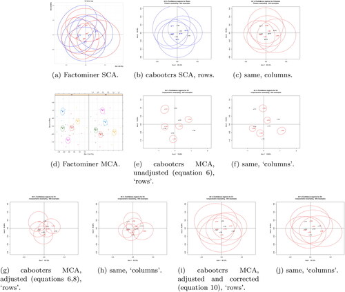
In Figure 1 it can clearly be seen that both SCA methods produce very similar results, both showing extensive overlap of regions as expected and required. In contrast, it can clearly be seen that both Factominer and MCA with unadjusted singular values (Eq. (6)(6) $${\mathit{d}}_j^{\star T}=({\mathit{c}}_j^{\star T}-{\mathit{c}}_j^T)D_{\mathit{r}}^{\star -\frac{1}{2}}[{\mathit{u}}_{(1)}^{\star } {\mathit{u}}_{(2)}^{\star }]j=1\dots J$$(6) only) produce much smaller regions, all showing clear separation. Table 1 gives the areas of the ellipses shown in Figure 1 in order to confirm these points. Note that Factominer output does not provide enough information to calculate the areas exactly, but the above results can be seen graphically in Figure 1.

Table 1. Areas of ellipses for completely random data shown in Figure 1.

Method	X11	X12	X13	X14	X15	X21	X22	X23	X24	X25
SCA	0.71	0.64	0.50	0.49	0.48	0.52	0.61	0.44	0.51	0.64
MCA unadjusted	0.20	0.16	0.12	0.13	0.12	0.13	0.16	0.11	0.14	0.18
MCA adjusted	0.18	0.17	0.12	0.13	0.12	0.14	0.15	0.11	0.14	0.16
MCA corrected	0.77	0.63	0.56	0.57	0.51	0.60	0.61	0.47	0.54	0.60

The data are random numbers and yet these pictures, either without confidence regions or with these small confidence regions, could mislead the user into thinking that there were genuine differences between the categories. However, MCA with adjusted singular values and the new correction by $p/(p-1)=2$ (Eq. (10)(10) $${\mathit{d}}_j^{\star \star T}=\frac{p}{p-1}({\mathit{c}}_j^{\star T}-{\mathit{c}}_j^T)D_{\mathit{r}}^{\star -\frac{1}{2}}[{\mathit{u}}_{(1)}^{\star } {\mathit{u}}_{(2)}^{\star }]j=1\dots J$$(10) ) produces ellipses that are very similar to those produced for SCA, showing the expected extensive overlap of regions, as can be seen graphically in Figure 1 and numerically in Table 1. MCA with adjusted singular values, but not the new correction, gives standard deviations of half the size and so produces ellipses of intermediate size relative to the scaling of the figure. Figure 1 shows that with adjusted singular values only the ellipses overlap substantially, even though Table 1 shows that the ellipses are approximately the same size as those with unadjusted singular values.

It can of course be argued that MCA should not really be applied to completely random data with p = 2, but this example clearly shows the inconsistency in conclusions between SCA and unadjusted MCA for a case where both can be applied to the same data.

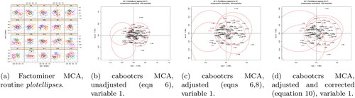
We can similarly generate a random data matrix X_np with $p=4,n=200,J_k=5,$ with results shown in Figure 2. As before, Factominer and MCA with unadjusted singular values (Eq. (6)(6) $${\mathit{d}}_j^{\star T}=({\mathit{c}}_j^{\star T}-{\mathit{c}}_j^T)D_{\mathit{r}}^{\star -\frac{1}{2}}[{\mathit{u}}_{(1)}^{\star } {\mathit{u}}_{(2)}^{\star }]j=1\dots J$$(6) only) produce visually very similar results, subject to the differences between use of the indicator and Burt matrices respectively. This time there is some overlap of regions, but again a user would be led to believe that there are genuine differences between the categories, even though the data are entirely ‘noise’. Using adjusted singular values produces regions which are larger relative to the rescaled coordinates. Only when using adjusted singular values and the correction by $p/(p-1)=4/3$ (Eq. (10)(10) $${\mathit{d}}_j^{\star \star T}=\frac{p}{p-1}({\mathit{c}}_j^{\star T}-{\mathit{c}}_j^T)D_{\mathit{r}}^{\star -\frac{1}{2}}[{\mathit{u}}_{(1)}^{\star } {\mathit{u}}_{(2)}^{\star }]j=1\dots J$$(10) ) are the regions as large and with as much overlap as we would have expected a priori, knowing that the data lack any structure.

Figure 2. Multiple CA CRs for completely random p = 4 data using factominer and cabooctrs R packages.

Although random data sets always show similar results, it should be noted that the Factominer and unadjusted regions show more of the expected overlaps when n is smaller relative to p, while of course the correction by $p/(p-1)$ makes less difference when p is larger. This can be seen with a final illustrative example with $p=20,n=50,J_k=5,$ with selected results shown in Figure 3. There is now much more of the expected overlap in the Factominer and unadjusted regions and there is less difference between the different methods, with observed differences mostly due to the randomness of the bootstrap and axis rearranging algorithm being exacerbated in such cases.

Figure 3. Multiple CA CRs for completely random p = 20 data using factominer and cabooctrs R packages.

An important caveat to all of the above is that, in simulations similar to those in Sec. 6.2, it was found that, when the method proposed here was applied to data with low or no correlation similar to the above, the ellipses for larger p tended to be too large. This is discussed further in Sec. 6.2.

5.2. Data with known structure

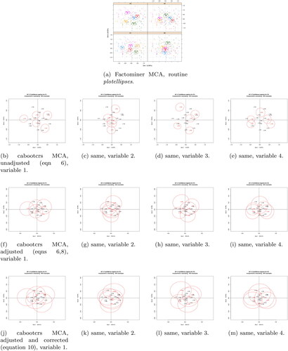
The connection between various forms of CA and generalized linear models (GLM) is well-known and described for the MCA case in Fithian and Josse (2017). Here we illustrate the connection using a very simple simulated data set constructed with p − 1 variables generated randomly as in Sec. 5.1 and a single two-category variable generated using a specified GLM with binomial errors and logit link. Hence we would expect a GLM fit to reproduce approximately the known generating model, while MCA CRs for the two-category variable and for variables with non-zero parameters in the generating model should be reasonably well separated and CRs for variables with parameters of zero should show substantial overlap.

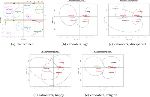
Here we show one illustrative example for p = 5 with $J_1=\dots =J_4=3,J_5=2$ and where the final two-category variable (Y) depends only on the fourth (X4). Hence we would expect clear differences between categories only for these last two variables. A GLM fit reproduces the generating model with only the categories of X4 being ‘significant’ as expected. Figure 4 shows the graphical results applying the corrected version of the proposed method and Factominer to these simulated data, from which can be seen that the results for the former are in line with prior expectation while those from the latter are not. This has been picked as a fairly typical example, with results being similar for other p and with more variables having non-zero parameters in the generating model.

Figure 4. MCA CRs for p = 5 data when only Y and X4 categories should differ, using factominer and cabooctrs R packages.

The differences in the Factominer results may be due to use of a partial bootstrap as well as the unadjusted scaling. A further important caveat is that this very limited set of illustrative examples does not show that the results for the Factominer plotellipses function are wrong, as that would depend on their objectives. All these examples show is that, in the limited number of cases investigated, the results from the corrected version of the method proposed here are closer to what would be expected.

6. Simulation study of performance

The proposed method is assessed by simulation according to its own criteria, so a key outcome is that when population profiles are projected as supplementary points onto sample axes they are indeed within the 95% confidence ellipse in approximately 95% of simulated samples.

6.1. Design

The simulation experiment is a full factorial design with four input factors, namely sample size (3 levels), number of variables (4 levels), number of categories per variable (3 levels) and structure of the population data matrix (3 levels). For each combination of levels a population of $N={10}^6$ individuals was randomly generated according to the above, then 1000 samples of the appropriate size drawn from this population (without replacement in each sample, with replacement over all samples) and the proposed method applied to each sample, using b = 999 bootstrap replicates.

The levels for the first three factors are n = 100, 250, 500, $p=4,8,16,24$ and categories per variable = 5, 7, 10. The 3 levels for the structure of the population matrix are defined as follows.

1. a random population correlation matrix is produced using the R randcorr routine Schmidt and Makalic (2018) and the data are generated as multivariate normal with this correlation matrix, then converted to categorical in such a way that all variable categories occur roughly equally often. The largest correlation in these random correlation matrices in fact tends to decrease with p. This produces data sets with little structure and a large number of small singular values, especially for larger p.

2. a $p\times 3$ matrix A of independent N(0, 1) variates is generated and the covariance matrix AA^T is made full rank by adding independent U(0, 1) variates to the diagonal, this is then standardized in the usual way to become the population correlation matrix and then used to produce categorical data as above. This produces data sets with moderately strong correlations (associations, structure) and a few moderately large singular values.

3. the first three columns of the population matrix are generated as completely random discrete uniform variates, then the others are generated as random perturbations and reflections of a random choice of one of the first three. This produces highly correlated (associated, structured) data sets, with the points often exhibiting the well-known horseshoe effect.

These will hereafter be referred to as the low, medium and high correlation cases, respectively.

The design is clearly imperfect and simplified to avoid a combinatorial explosion. It can be argued that there should be varying numbers of categories in each case, or that the sample size should be relative to the number of variables and categories, or that the correlations between variables in fact decrease and increase with p in the first and third cases respectively.

The main outputs used here are the observed inclusion rates (IRs) of population points within the confidence regions for the first two sample axes, compared to the nominal 90, 95 and 99% values. Only the first two sample axes are considered as these are the only axis pair which will, in practice, be used in all analyses. The other main output used is the accuracy and precision with which the bootstrap variance matrices estimate the true variance matrices.

The N by p population matrix is used to derive directly the population profiles $C^{‡},$ while MCA is applied to it to calculate the population axes. Inclusion rates are then estimated over all categories in all variables, by projecting the appropriate population column profile point, i.e. row of $C^{‡},$ onto the first two sample axes and checking whether it is inside or outside the confidence ellipse.

The true variance matrices are estimated by projecting the difference between the appropriate sample and population profile points, i.e. row of $C-C^{‡},$ onto the sample axes, which have been rearranged to correspond to the population axes. The 1000 samples then allow estimation of the true variance matrices for the sample axes corresponding to the first two population axes. Hence note that the IRs are calculated for the first two sample axes in each sample, whereas the variances are calculated using the sample axes corresponding to the first two population axes. These may not be the same, especially in samples where the first few singular values are close.

All simulations were run in R using Rstudio on a Lenovo Thinkpad with Intel i7 running Ubuntu linux.

6.2. Results

The empirical inclusion rate results were analyzed using a generalized linear model with binomial errors and logit and probit links, showing that the results were clearly overdispersed compared to the binomial, as is commonly the case with many data sets. The sample sizes in the simulation were sufficiently large that all main effect and most estimable interaction parameters in the model were ‘significant’, and the nature of the differences and the overdispersion are most easily seen in simple boxplots.

It was fairly clear from the above analysis and from preliminary plots that the correlation/association level is the most important factor and the number of categories per variable the least important, so that all boxplots collapse over the latter. Each point on the boxplots in Figure 5 is one category of one variable, so that there are 22p points making up each column of each boxplot, while each point is calculated based on 1000 samples from the same simulated population.

Figure 5. Proportion of 95% ellipses containing the population point, over 1000 simulations.

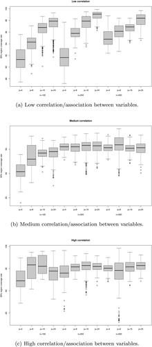
Critical values estimated with bootstrapping performed consistently slightly better than ${\chi }_2^2$ critical values, so only the former will be reported. Results for nominal coverage rates other than 95% show a very similar pattern to those for 95%, hence only these are shown.

As seen in Figure 5, in the medium and high correlation cases the method performs reasonably well according to its own criteria. In most cases the interquartile range is fairly narrow and includes the nominal coverage rate of 95%, while the empirical inclusion rate only goes below 90% in a fairly small number of cases.

The main cause of concern is the very high empirical inclusion rate for p = 24 in the low correlation case, i.e. when correlation matrices were generated with randcorr, and the clear implication that inclusion rates increase with p in this case. This is probably because, as p increases, the axis rearranging approach does not remove enough of the spurious variation mentioned in Sec. 4.2, so that estimated variances, and hence ellipse sizes, are too large. It was found in preliminary simulations that this tended to happen when the method was applied either to data with very low correlation or to completely random data with no correlation, as in Sec. 5.1. In such cases there is very little structure in the data so that the singular values are very close and hence the singular vectors both reorder and rotate substantially from sample to sample. In such cases the Procrustes rotation approach might perform better, but here we retain the axis rearrangement approach for the reasons explained in Ringrose (2012, 1996). For the simulated data generated using randcorr for p = 24, just under half of the two-way contingency tables which make up the Burt matrices had p-values under 5%, suggesting very low structure. However, it is arguable that in these cases of very low structure/correlation it is preferable to err on the side of confidence regions being too large rather than too small, as these are less likely to mislead the user into over-interpreting random noise, as illustrated in Sec. 5.1.

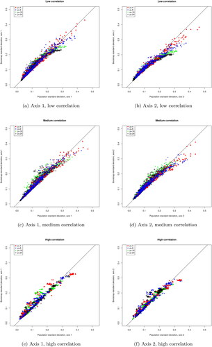
Figure 6 shows plots of the bootstrap standard deviations against the estimated population standard deviations. Here we see in all cases a tendency for small to medium standard deviations to be overestimated more often than underestimated, while the small number of larger standard deviations are more likely to be underestimated, especially on the second axis and in the low correlation case. The high simulated inclusion rates in the low correlation case, seen in Figure 5, hence seem to be caused mostly by the smaller ellipses being too large. However, despite the noticeable curve in the plots, a large number of points are very close to the identity line, albeit often just above it. Although assessing the precision of the estimates of the variance matrix helps to interpret the other results, it is difficult to say what constitutes good or poor precision in this case. Hence performance is judged here mostly in terms of whether the nominal coverage rates of the ellipses are approximately met, and whether a statistically literate user would be led toward reasonable conclusions about the presence or otherwise of differences between the categories of the variables.

Figure 6. Bootstrap versus estimated population standard deviations for first two population axes.

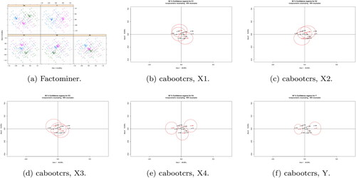
7. Example

The proposed approach is illustrated on a small data set, again on the principle that a key feature of any confidence statement is to prevent the overinterpretation of random noise. The data in Takane and Hwang (2006, table 11.1) (originally in Nishisato (1994)) are the results of a small survey with n = 23 and p = 4, where the questions are age, whether the respondent thinks that children or less disciplined and less happy than in the past, and whether religion should be taught in schools. The plotted confidence regions in Figure 7 show that once again those produced by the proposed method are mostly rather larger than those from Factominer Lê, Josse, and Husson (2008), noting again that the former uses the adjusted coordinates from the Burt matrix while the latter uses the indicator matrix, and also larger than those given in Takane and Hwang (2006). In this case there is no known ‘correct’ answer, but with n = 23 the regions produced by the proposed method seem more in line with what would be expected.

Figure 7. MCA CRs for nishisato’s small survey data, with factominer and cabootcrs.

8. Conclusions

Multiple correspondence analysis, in various guises, is a widely used method for graphically investigating multidimensional categorical data. The danger with any purely graphical exploratory method is that, without error bars or similar, it can lead to the overinterpretation of what is in fact random variation. The proposed method has been shown by simulation to perform reasonably well in the cases considered, although inevitably a huge variety of data structures and sizes have not yet been investigated. It has also been shown by simulation that, in the special cases considered, the corrected version of the proposed method produced graphical results in line with what the user would expect, whereas those produced by the uncorrected version often did not.

Two obvious weaknesses of the approach proposed here are that it does not deal with either the indicator matrix or with ordinal data. These, and the apparent poor performance on data with low structure, are topics for future research.

Notes

All of the methods proposed are implemented in the R package cabootcrs Ringrose (2022), available from CRAN.

Disclosure statement

No potential conflict of interest was reported by the author(s).

References

- Alzahrani, A. A., E. J. Beh, and E. Stojanovski. 2023. Confidence regions for simple correspondence analysis using the Cressie-Read family of divergence statistics. Electronic Journal of Applied Statistical Analysis 16:423–48.
- Beh, E. J. 2010. Elliptical confidence regions for simple correspondence analysis. Journal of Statistical Planning and Inference 140 (9):2582–8. doi:10.1016/j.jspi.2010.03.018.
- Beh, E. J., and R. Lombardo. 2015. Confidence regions and approximate p-values for classical and non symmetric correspondence analysis. Communications in Statistics - Theory and Methods 44 (1):95–114. doi:10.1080/03610926.2013.768665.
- Berkelaar, M. 2023. Interface to Lp_solve v. 5.5 to solve linear/integer programs. https://cran.r-project.org/package=lpSolve (accessed June 2023).
- Corral-De-Witt, D., E. Carrera, S. Muñoz-Romero, K. Tepe, and J. Rojo-Álvarez. 2019. Multiple correspondence analysis of emergencies attended by integrated security services. Applied Sciences 9 (7):1396. doi:10.3390/app9071396.
- D’Ambra, A., and P. Amenta. 2023. An extension of correspondence analysis based on the multiple Taguchi’s index to evaluate the relationships between three categorical variables graphically: An application to the Italian football championship. Annals of Operations Research 325 (1):219–44. doi:10.1007/s10479-022-04803-3.
- D’Ambra, A., P. Amenta, and E. J. Beh. 2021. Confidence regions and other tools for an extension of correspondence analysis based on cumulative frequencies. AStA Advances in Statistical Analysis 105 (3):405–29. doi:10.1007/s10182-020-00382-5.
- D'Ambra, A., and A. Crisci. 2014. The confidence ellipses in decomposition multiple non symmetric correspondence analysis. Communications in Statistics - Theory and Methods 43 (6):1209–21. doi:10.1080/03610926.2012.667487.
- Davison, A. C., and D. V. Hinkley. 1997. Bootstrap methods and their applications. Cambridge: Cambridge University Press.
- Di Franco, G. 2016. Multiple correspondence analysis: One only or several techniques? Quality & Quantity 50 (3):1299–315. doi:10.1007/s11135-015-0206-0.
- Fithian, W., and J. Josse. 2017. Multiple correspondence analysis and the multilogit bilinear model. Journal of Multivariate Analysis 157:87–102. doi:10.1016/j.jmva.2017.02.009.
- Gifi, A. 1990. Nonlinear multivariate analysis. Chichester: Wiley.
- González-Serrano, L., P. Talón-Ballestero, S. Muñoz-Romero, C. Soguero-Ruiz, and J. L. Rojo-Álvarez. 2020. A big data approach to customer relationship management strategy in hospitality using multiple correspondence domain description. Applied Sciences 11 (1):256–74. doi:10.3390/app11010256.
- Greenacre, M. J. 1984. Theory and applications of correspondence analysis. London: Academic Press.
- Greenacre, M. J. and J. Blasius, eds. Multiple correspondence analysis and related methods. Boca Raton, FL: Chapman and Hall, 2006.
- Iacobucci, D., and D. Grisaffe. 2018. Perceptual maps via enhanced correspondence analysis: Representing confidence regions to clarify brand positions. Journal of Marketing Analytics 6 (3):72–83. doi:10.1057/s41270-018-0037-7.
- Lê, S., J. Josse, and F. Husson. 2008. Factominer: A package for multivariate analysis. Journal of Statistical Software 25 (1):1–18. doi:10.18637/jss.v025.i01.
- Lebart, L. 2006. Validation techniques in multiple correspondence analysis. In Multiple correspondence analysis and related methods, ed. M. J. Greenacre and J. Blasius, 179–95. Boca Raton, FL: Chapman and Hall.
- Lebart, L. 2007a. Which bootstrap for principal axes methods? In Selected contributions in data analysis and classification, ed. P. Brito, G. Cucumel, P. Bertrand, and F. de Carvalho, 581–8. Berlin: Springer.
- Lebart, L. 2007b. Confidence areas for planar visualizations through partial and procrustean bootstrap, with application to textual data. https://www.researchgate.net/profile/Ludovic-Lebart/publication/228825459_Confidence_areas_for_planar _visualizations_through_partial_and _procrustean_bootstrap_with_application_to_textual_data/links/5628cf4208aef25a243d2240/Confidence-areas-for-planar-visualizations-through-partial -and-procrustean-bootstrap-with-application-to-textual-data.pdf (accessed June 2023).
- Lebart, L., A. Morineau, and K. M. Warwick. 1984. Multivariate descriptive statistical analysis. New York: Wiley.
- Markus, M. T. 1994a. Bootstrap confidence regions for homogeneity analysis; the influence of rotation on coverage percentages. In COMPSTAT: Proceedings in Computational Statistics: 11th Symposium, Vienna, Austria, ed. R. Dutter and W. Grossmann, 337–342. Heidelberg: Physica-Verlag.
- Markus, M. T. 1994b. Bootstrap confidence regions in non-linear multivariate analysis. Leiden: DSWO Press.
- Michailidis, G., and J. de Leeuw. 1998. The Gifi system of descriptive multivariate analysis. Statistical Science 13 (4):307–36. doi:10.1214/ss/1028905828.
- Milan, L., and J. Whittaker. 1995. Application of the parametric bootstrap to models that incorporate a singular value decomposition. Applied Statistics 44 (1):31–50. doi:10.2307/2986193.
- Nishisato, S. 1994. Elements of dual scaling: An introduction to practical data analysis. New Jersey: Lawrence Erlbaum Associates.
- Ringrose, T. J. 1992. Bootstrapping and correspondence analysis in archaeology. Journal of Archaeological Science 19 (6):615–29. doi:10.1016/0305-4403(92)90032-X.
- Ringrose, T. J. 1994. Bootstrap confidence regions for canonical variate analysis. In COMPSTAT: Proceedings in Computational Statistics: 11th Symposium, Vienna, Austria, ed. R. Dutter and W. Grossmann, 343–348. Heidelberg: Physica-Verlag.
- Ringrose, T. J. 1996. Alternative confidence regions for canonical variate analysis. Biometrika 83 (3):575–87. doi:10.1093/biomet/83.3.575.
- Ringrose, T. J. 2012. Bootstrap confidence regions for correspondence analysis. Journal of Statistical Computation and Simulation 82 (10):1397–413. doi:10.1080/00949655.2011.579968.
- Ringrose, T. J. 2022 March. Bootstrap confidence regions for simple and multiple correspondence analysis. https://cran.r-project.org/package=cabootcrs.
- Schmidt, D. F., and E. Makalic. 2018. Randcorr: Generate a random p × p correlation matrix. https://cran.r-project.org/package=randcorr (accessed June 2023).
- Sharpe, J., and N. Fieller. 2016. Uncertainty in functional principal component analysis. Journal of Applied Statistics 43 (12):2295–309. doi:10.1080/02664763.2016.1140728.
- Takane, Y., and H. Hwang. 2006. Regularised multiple correspondence analysis. In Multiple correspondence analysis and related methods, ed. M. J. Greenacre and J. Blasius, 259–79. Boca Raton, FL: Chapman and Hall.