An empirical study of the durbin and ANOVA F tests and their contrasts

Abstract

The Durbin and ANOVA F test on the ranks are competing tests for equality of treatment mean ranks. When the levels of the treatments are ordered, both tests have informative decompositions into orthonormal contrasts that detect linear, quadratic, etc. effects. It is known that the ANOVA F test on the ranks better adheres to the nominal significance level than the Durbin test. Here we investigate whether the same is true for their orthonormal contrasts.

Keywords:

• Helmert contrasts
• Nonparametric testing
• Ranks
• Test sizes

MATHEMATICAL SUBJECT CLASSIFICATION:

• 62G
• 62F

1. Introduction

Best and Rayner (2014) gave an empirical study of the Durbin and ANOVA F test on the ranks when treatments are ordered. They gave test sizes and powers and conjectured that power differences were due to size differences. Rayner and Livingston Jr (2023a, Sec. 5.3) showed there is a 1–1 relationship between the two test statistics, so the conjecture is true. The empirical study showed that in general the F test gave test sizes closer to the nominal 0.05 than the Durbin test.

Thas, Best, and Rayner (2012) showed how to construct orthonormal contrasts for Durbin’s test, while Rayner and Livingston Jr (2023b) did likewise for the ANOVA F test on the ranks. Here we investigate how well the test sizes of the orthonormal contrasts of the Durbin and ANOVA F test on the ranks adhere to their nominal test size. Does the superiority of the ANOVA F test on the ranks extend to the contrasts?

In the next section contrasts and the tests are defined. In section three the empirical study is reported. An example of the application of the tests is given in Sec. 5. A brief conclusion follows.

2. The tests and their contrasts

We begin by defining orthonormal contrasts. Suppose Y = (Y₁, …, Y_t)^T is a vector of random variables and c = (c₁, …, c_t)^T is a vector of constants. For i = 1, …, t suppose Y_i is the sum of n_i observations, that n = ${\sum }_i{n}_i,$ and that p_i = n_i/n. Then c^TY is a contrast in Y if and only if p₁c₁ + …+ p_tc_t = 0.

In general a weight function is a set {p_i} in which p_i > 0 for i = 1, …, t and ${\sum }_i{p}_i$ = 1. Suppose $\left\{h_u\right\}$ is orthonormal with weight function {p_i}. Here h_u = (h_u1, …, h_ut)^T for u = 1, …, t. Orthonormality means that E $\left[h_u^{\mathrm{T}}{h}_v\right]={\delta }_{\mathit{\text{uv}}},$ the Kronecker delta in which the expectation is with respect to the distribution with probability function {p_i}. It is customary to take the orthonormal function of degree zero to be identically 1 and here we designate h_t to be this function.

The orthonormality and choice of h_t means that for u = 1, …, t − 1, ${\mathrm{E}[h}_t^{\mathrm{T}}{h}_u]={\delta }_{\mathit{\text{ut}}}={\sum }_i{h}_{\mathit{\text{ui}}}{p}_i=0.$ It follows that with p_i = n_i/n, i = 1, …, t, the $h_u^{\mathrm{T}}Y$ = ${\sum }_i{h_{\mathit{\text{ui}}}p}_i{Y}_i$ are contrasts. Coupled with their orthonormality, we say the $h_u^{\mathrm{T}}Y$ are orthonormal contrasts with weight function {p_i}.

In the balanced incomplete block design each of the b blocks contains k experimental units, each of the t treatments appears in r blocks, and every treatment appears with every other treatment precisely λ times. Necessarily $$k<t,r<b,\mathit{\text{bk}}=\mathit{\text{rt}},\text{and}\lambda (t-1)=r(k-1).$$

Treatments are ranked within each block. Such a design will be designated BIBD (t, b, k, r).

If ties occur and ranks are assigned so that the rank sums are not affected, then an adjusted Durbin test statistic is given by $$D_{\mathrm{A}}=\frac{\left(t-1\right)\{{\sum }_i{R}_i^2-\frac{\mathit{\text{rbk}}{\left(k+1\right)}^2}{4}\}}{{\sum }_{i,\mathrm{j}}{r}_{\mathit{\text{ij}}}^2-\frac{\mathit{\text{bk}}{\left(k+1\right)}^2}{4}}$$ in which r_ij is the rank of treatment i on block j, and R_i = ${\sum }_j{r}_{\mathit{\text{ij}}}$ is the sum of the ranks given to treatment i, i = 1, …, t and j = 1, …, b. If there are no ties then on block j the ranks are 1, 2, …, k so that ${\sum }_{i,j}{r}_{\mathit{\text{ij}}}^2$ = bk(k + 1)(2k + 1)/6 and the denominator in D_A is b(k − 1)k(k + 1)/12.

Rayner and Livingston Jr (2023a, Sec. 5.3) show that when there are ties that preserve the rank sum, the ANOVA F test statistic on the ranks, F say, is related to the adjusted Durbin statistic D_A by $$F=\frac{\mathit{\text{edf}}\mathrm{ }{D}_{\mathrm{A}}}{(t-1)\left\{b\right(k-1)-D_{\mathrm{A}}\}}$$ in which edf = bk – b – t + 1, the error degrees of freedom.

Rayner and Livingston Jr (2023a) show that if $Z_i=(R_i-E[R_i])/\sqrt{{\sum }_j{S}_j}$ in which $$S_j={\sum }_i{r}_{\mathit{\text{ij}}}^2/b_j-{\left({\sum }_i{r}_{\mathit{\text{ij}}}\right)}^2/b_j^2,$$

the variance of the ranks on the jth block, then $h_u^{\mathrm{T}}Z\sqrt{r(t-1)/k}=h_u^{\mathrm{T}}Z\sqrt{b(t-1)/t},$ for u = 1, …, t − 1 are orthonormal contrasts whose sum of squares is D_A. Here {h_u} is orthonormal with respect to the weight function p_j = 1/t, j = 1, …, t. These are the Legendre polynomials and for programming purposes can be conveniently programmed using the recurrence given in Rayner, Thas, and De Boeck (2008).

Now consider a fixed effects ANOVA design with multiple factors. The observations are mutually independent and normally distributed with constant variance ${\sigma }^2.$ Suppose Y_ij is the jth of n_i observations of the ith of r levels of factor A. There are n = ${\sum }_i{n}_i$ observations in all and ultimately but not immediately we assume the levels of A are ordered. Write $Y_{i.}$ for the sum of the observations for level i, and ${\overline{Y}}_{i.}$ for the mean of same.

Under the null hypothesis of no factor A effect, the factor sum of squares, SS_F = ${\sum }_i{n_i({\overline{Y}}_{i.}-{\overline{Y}}_{.})}^2$ = ${\sum }_i{Y}_{i.}^2/n_i$ – $Y_{.}^2/n,$ has the ${\sigma }^2{\chi }_{r-1}^2$ distribution. Write Z = ((${\overline{Y}}_{1.}-{\overline{Y}}_{.})\sqrt{n_1},$ …, (${\overline{Y}}_{r.}-{\overline{Y}}_{.})\sqrt{n_r}$)^T.

Suppose that m₁, …, m_r–1 are any orthonormal vectors and write SS_E for the error sum of squares, and edf for the corresponding error degrees of freedom. Rayner and Livingston Jr (2023b) show that the ($m_u^{\mathrm{T}}Z$)²/{SS_E/edf} = F_u say, are mutually independent and F_1,edf distributed.

We now show how to choose the {m_u}. Suppose h₁, …, h_r are orthonormal with weight function {p_i}, so that ${\sum }_i{h}_{\mathit{\text{ui}}}{h_{\mathit{\text{vi}}}p}_i={\delta }_{\mathit{\text{uv}}}.$ Take p_i = n_i/n and put m_ui = $h_{\mathit{\text{ui}}}\sqrt{p_i}.$ Then (m_ui) is an orthogonal matrix and the $m_u^{\mathrm{T}}Z$ are orthonormal contrasts. For ordered treatments the {h_u} may be chosen to be the orthonormal polynomials on the weight function {n_i/n} with the degree zero polynomial identically one. The resulting contrasts can reasonably be called ordered F contrasts. When the treatment levels are not ordered the scenario will suggest which comparisons are of interest. However a fall-back is to use a Helmert matrix, for which see Lancaster (1965). Examples are given in Rayner and Livingston Jr (2023c).

3. The empirical study

Here we will consider the same BIBDs (b, k, r, t) as did Best and Rayner (2014), mainly so we can compare our results with theirs. Because we analyze additional distributions to generate our data than they do, we will consider two randomly chosen designs more deeply than the rest. In Best and Rayner (2014), the data sets are generated from a discrete uniform distribution, DU(1, $k$), with probability mass function $p_l=1/k$ for $l=1,\dots ,k.$ That was so that as the designs tended to get larger, the number of possible values the response variable could take was increased. The proportions of exceedances using the appropriate ${\chi }^2$ and F critical points and 100,000 simulations on each design were calculated.

Here, we generate data from several distributions across the different designs: the continuous uniform; DU (1, 3); DU (1, 5); DU (1, 7); and beta distributions with parameters (0.2, 0.8); (0.5, 0.5); and, (1, 5). The discrete uniform distributions are to reflect categorization of varying degrees and hence the prevalence of ties. The beta distribution parameters are selected to ensure a variety of shapes. For all designs and data generating distributions, the test sizes based on the ${\chi }^2$ and F distributions are from 1,000,000 simulations. For the permutation test sizes, these are based on 100,000 simulations each with 100,000 permutations and are presented in parentheses in the tables. Test sizes outside of (0.02, 0.09) have been set in boldface. For each of the tables in this section, D and F refer to tests of overall effects, where as D_i and F_i refer to testing for ith degree polynomial effects.

Best and Rayner (2014), state that infrequently, the error sum of squares is zero, and the simulated data was discarded when this was the case. Here we do not discard the data, but instead naively apply the F tests using an error sum of squares of zero. For overall effects this results in a p-value of zero. For the contrasts, there are occasionally zero divided zero calculations for the test statistic of the contrast, when this is the case we take the p-value to be 1. These situations rarely occur and do so only for the discrete uniform distributions. We provide counts of the number of times this happens for each of the designs. A second difference between our work and that of Best and Rayner (2014) is in the treatment of ties. Also, it appears that the description of Table 1 in Best and Rayner (2014) might not reflect what is actually shown in the table. The text states that the table shows test sizes calculated using permutation tests. We suggest that if that were the case, the test sizes for the Durbin and F tests should be the same due the one-to-one relationship between the test statistics. It appears to us that these test sizes are from tests comparing the test statistics to ${\chi }^2$ or F distributions.

Table 1. Simulated test sizes for the Durbin and ANOVA F tests and their contrasts for the BIBD (3, 7) when sampling from various distributions.

Durbin	D	D1	D2	D3	D4	D5	D6
U(0, 1)	0.0000 (0.0420)	0.0529 (0.0462)	0.0471 (0.0499)	0.0413 (0.0484)	0.0455 (0.0494)	0.0465 (0.0480)	0.0373 (0.0505)
DU(1, 3)	0.0017 (0.0404)	0.0465 (0.0462)	0.0470 (0.0491)	0.0450 (0.0484)	0.0472 (0.0482)	0.0466 (0.0488)	0.0455 (0.0495)
DU(1, 5)	0.0009 (0.0443)	0.0473 (0.0488)	0.0485 (0.0492)	0.0469 (0.0482)	0.0472 (0.0501)	0.0480 (0.0496)	0.0450 (0.0498)
DU(1, 7)	0.0005 (0.0441)	0.0472 (0.0483)	0.0486 (0.0489)	0.0466 (0.0493)	0.0473 (0.0504)	0.0479 (0.0497)	0.0440 (0.0498)
B(0.2, 0.8)	0.0000 (0.0425)	0.0526 (0.0486)	0.0466 (0.0495)	0.0412 (0.0484)	0.0454 (0.0496)	0.0460 (0.0497)	0.0377 (0.0505)
B(0.5, 0.5)	0.0000 (0.0422)	0.0527 (0.0467)	0.0470 (0.0490)	0.0411 (0.0494)	0.0451 (0.0502)	0.0465 (0.0500)	0.0377 (0.0486)
B(5, 1)	0.0000 (0.0417)	0.0525 (0.0477)	0.0467 (0.0498)	0.0410 (0.0488)	0.0455 (0.0496)	0.0467 (0.0501)	0.0373 (0.0500)
ANOVA F	F	F1	F2	F3	F4	F5	F6
U(0, 1)	0.0887 (0.0420)	0.0559 (0.0486)	0.0566 (0.0508)	0.0526 (0.0499)	0.0550 (0.0501)	0.0567 (0.0495)	0.0555 (0.0507)
DU(1, 3)	0.0609 (0.0404)	0.0551 (0.0501)	0.0547 (0.0492)	0.0544 (0.0499)	0.0547 (0.0479)	0.0548 (0.0480)	0.0541 (0.0490)
DU(1, 5)	0.0648 (0.0443)	0.0558 (0.0503)	0.0555 (0.0496)	0.0561 (0.0504)	0.0555 (0.0510)	0.0557 (0.0490)	0.0556 (0.0493)
DU(1, 7)	0.0654 (0.0441)	0.0554 (0.0501)	0.0556 (0.0495)	0.0560 (0.0507)	0.0557 (0.0501)	0.0555 (0.0503)	0.0556 (0.0496)
B(0.2, 0.8)	0.0892 (0.0425)	0.0555 (0.0501)	0.0565 (0.0490)	0.0528 (0.0490)	0.0548 (0.0497)	0.0561 (0.0506)	0.0559 (0.0501)
B(0.5, 0.5)	0.0889 (0.0422)	0.0560 (0.0489)	0.0567 (0.0497)	0.0524 (0.0501)	0.0548 (0.0496)	0.0567 (0.0509)	0.0556 (0.0496)
B(5, 1)	0.0887 (0.0417)	0.0558 (0.0499)	0.0564 (0.0497)	0.0525 (0.0504)	0.0549 (0.0489)	0.0570 (0.0502)	0.0552 (0.0498)

The first test size in each cell is for tests using the ${\chi }^2$ or F distributions, the second from permutation tests.

For the BIBD (7, 33) in Table 1 and BIBD (3, 4) in Table 2, the results vary little across the distributions sampled indicating that the tests are truly nonparametric. For the other designs considered in Tables 3–12 we only give results for data generated from the continuous uniform and discreet uniform distributions.

Table 2. Simulated test sizes for the Durbin and ANOVA F tests and their contrasts for the BIBD (3, 4) when sampling from various distributions.

Durbin	D	D1	D2	D3
U(0, 1)	0.0000 (0.0183)	0.0345 (0.0342)	0.0253 (0.0249)	0.0343 (0.0499)
DU(1, 3)	0.0021 (0.0262)	0.0462 (0.0362)	0.0514 (0.0233)	0.0461 (0.0407)
DU(1, 5)	0.0004 (0.0325)	0.0470 (0.0414)	0.0523 (0.0311)	0.0471 (0.0466)
DU(1, 7)	0.0002 (0.0311)	0.0459 (0.0427)	0.0479 (0.0325)	0.0460 (0.0478)
B(0.2, 0.8)	0.0000 (0.0194)	0.0348 (0.0342)	0.0251 (0.0251)	0.0345 (0.0494)
B(0.5, 0.5)	0.0000 (0.0188)	0.0347 (0.0348)	0.0251 (0.0249)	0.0348 (0.0499)
B(5, 1)	0.0000 (0.0190)	0.0346 (0.0354)	0.0250 (0.0244)	0.0345 (0.0501)
ANOVA F	F	F1	F2	F3
U(0, 1)	0.0756 (0.0183)	0.0863 (0.0491)	0.0442 (0.0432)	0.0862 (0.0492)
DU(1, 3)	0.0800 (0.0262)	0.0628 (0.0425)	0.0571 (0.0390)	0.0633 (0.0417)
DU(1, 5)	0.0845 (0.0325)	0.0687 (0.0477)	0.0613 (0.0434)	0.0687 (0.0477)
DU(1, 7)	0.0871 (0.0311)	0.0707 (0.0482)	0.0613 (0.0453)	0.0708 (0.0487)
B(0.2, 0.8)	0.0755 (0.0194)	0.0870 (0.0485)	0.0441 (0.0434)	0.0866 (0.0491)
B(0.5, 0.5)	0.0759 (0.0188)	0.0864 (0.0495)	0.0442 (0.0441)	0.0867 (0.0489)
B(5, 1)	0.0754 (0.0190)	0.0864 (0.0496)	0.0439 (0.0432)	0.0865 (0.0500)

The first test size in each cell is for tests using the ${\chi }^2$ or F distributions, the second from permutation tests.

Table 3. Simulated test sizes for the Durbin and ANOVA F tests and their contrasts for the BIBD (2–4, 6) when sampling from the U(0, 1) and DU(1, 3) distributions.

Durbin	D	D1	D2	D3
U(0, 1)	0.0000 (0.0000)	0.0310 (0.0307)	0.1254 (0.0000)	0.0311 (0.0317)
DU(1, 3)	0.0000 (0.0000)	0.0223 (0.0026)	0.0369 (0.0000)	0.0222 (0.0028)
ANOVA F	F	F1	F2	F3
U(0, 1)	0.0000 (0.0000)	0.0310 (0.0307)	0.1254 (0.0000)	0.0311 (0.0317)
DU(1, 3)	0.0198 (0.0000)	0.0730 (0.0026)	0.0819 (0.0000)	0.0729 (0.0028)

The first test size in each cell is for tests using the ${\chi }^2$ or F distributions, the second from permutation tests.

Table 4. Simulated test sizes for the Durbin and ANOVA F tests and their contrasts for the BIBD (2, 4, 5, 10) when sampling from the U(0, 1) and DU(1, 3) distributions.

Durbin	D	D1	D2	D3	D4
U(0, 1)	0.0000 (0.0000)	0.0642 (0.0274)	0.0320 (0.0407)	0.0640 (0.0347)	0.0558 (0.0476)
DU(1, 3)	0.0005 (0.0215)	0.0470 (0.0264)	0.0485 (0.0300)	0.0476 (0.0317)	0.0423 (0.0298)
ANOVA F	F	F1	F2	F3	F4
U(0, 1)	0.1199 (0.0000)	0.0741 (0.0421)	0.0639 (0.0484)	0.0740 (0.0467)	0.0798 (0.0508)
DU(1, 3)	0.0550 (0.0215)	0.0589 (0.0320)	0.0598 (0.0324)	0.0590 (0.0335)	0.0549 (0.0327)

The first test size in each cell is for tests using the ${\chi }^2$ or F distributions, the second from permutation tests.

Table 5. Simulated test sizes for the Durbin and ANOVA F tests and their contrasts for the BIBD (4, 5) when sampling from the U(0, 1) and DU(1, 3) distributions.

Durbin	D	D1	D2	D3	D4
U(0, 1)	0.0261 (0.0458)	0.0474 (0.0475)	0.0458 (0.0466)	0.0473 (0.0495)	0.0386 (0.0503)
DU(1, 3)	0.0258 (0.0477)	0.0468 (0.0469)	0.0482 (0.0481)	0.0466 (0.0508)	0.0472 (0.0479)
ANOVA F	F	F1	F2	F3	F4
U(0, 1)	0.0643 (0.0458)	0.0563 (0.0492)	0.0549 (0.0490)	0.0561 (0.0495)	0.0555 (0.0511)
DU(1, 3)	0.0617 (0.0477)	0.0543 (0.0504)	0.0541 (0.0496)	0.0543 (0.0510)	0.0542 (0.0497)

The first test size in each cell is for tests using the ${\chi }^2$ or F distributions, the second from permutation tests.

Table 6. Simulated test sizes for the Durbin and ANOVA F tests and their contrasts for the BIBD (3, 5, 6, 10) when sampling from the U(0, 1) and DU(1, 3) distributions.

Durbin	D	D1	D2	D3	D4
U(0, 1)	0.0343 (0.0419)	0.0547 (0.0486)	0.0472 (0.0480)	0.0548 (0.0496)	0.0424 (0.0466)
DU(1, 3)	0.0340 (0.0460)	0.0482 (0.0462)	0.0496 (0.0477)	0.0476 (0.0491)	0.0476 (0.0475)
ANOVA F	F	F1	F2	F3	F4
U(0, 1)	0.0609 (0.0419)	0.0522 (0.0496)	0.0491 (0.0489)	0.0521 (0.0504)	0.0534 (0.0493)
DU(1, 3)	0.0572 (0.0460)	0.0526 (0.0498)	0.0522 (0.0492)	0.0521 (0.0494)	0.0517 (0.0484)

The first test size in each cell is for tests using the ${\chi }^2$ or F distributions, the second from permutation tests.

Table 7. Simulated test sizes for the durbin and ANOVA F tests and their contrasts for the BIBD (2, 5, 6, 15) when sampling from the U(0, 1) and DU(1, 3) distributions.

Durbin	D	D1	D2	D3	D4	D5
U(0, 1)	0.0219 (0.0228)	0.0480 (0.0488)	0.0423 (0.0454)	0.0436 (0.0499)	0.0583 (0.0467)	0.0450 (0.0493)
DU(1, 3)	0.0140 (0.0325)	0.0477 (0.0389)	0.0477 (0.0360)	0.0473 (0.0463)	0.0488 (0.0456)	0.0457 (0.0481)
ANOVA F	F	F1	F2	F3	F4	F5
U(0, 1)	0.0512 (0.0228)	0.0491 (0.0486)	0.0524 (0.0462)	0.0560 (0.0489)	0.0565 (0.0501)	0.0531 (0.0489)
DU(1, 3)	0.0627 (0.0325)	0.0526 (0.0468)	0.0534 (0.0458)	0.0532 (0.0473)	0.0530 (0.0468)	0.0535 (0.0486)

The first test size in each cell is for tests using the ${\chi }^2$ or F distributions, the second from permutation tests.

Table 8. Simulated test sizes for the Durbin and ANOVA F tests and their contrasts for the BIBD (3, 5, 6, 10) when sampling from the U(0, 1) and DU(1, 3) distributions.

Durbin	D	D1	D2	D3	D4	D5
U(0, 1)	0.0263 (0.0444)	0.0466 (0.0472)	0.0584 (0.0411)	0.0487 (0.0489)	0.0508 (0.0494)	0.0471 (0.0499)
DU(1, 3)	0.0278 (0.0466)	0.0488 (0.0479)	0.0475 (0.0457)	0.0482 (0.0497)	0.0482 (0.0493)	0.0478 (0.0506)
ANOVA F	F	F1	F2	F3	F4	F5
U(0, 1)	0.0627 (0.0444)	0.0542 (0.0489)	0.0522 (0.0487)	0.0509 (0.0498)	0.0550 (0.0495)	0.0533 (0.0501)
DU(1, 3)	0.0583 (0.0466)	0.0517 (0.0502)	0.0526 (0.0492)	0.0523 (0.0493)	0.0527 (0.0498)	0.0523 (0.0508)

The first test size in each cell is for tests using the ${\chi }^2$ or F distributions, the second from permutation tests.

Table 9. Simulated test sizes for the Durbin and ANOVA F tests and their contrasts for the BIBD (3, 6, 10, 20) when sampling from the U(0, 1) and DU(1, 3) distributions.

Durbin	D	D1	D2	D3	D4	D5
U(0, 1)	0.0391 (0.0439)	0.0458 (0.0481)	0.0558 (0.0427)	0.0489 (0.0499)	0.0478 (0.0495)	0.0481 (0.0498)
DU(1, 3)	0.0407 (0.0488)	0.0487 (0.0474)	0.0488 (0.0478)	0.0490 (0.0487)	0.0494 (0.0492)	0.0488 (0.0510)
ANOVA F	F	F1	F2	F3	F4	F5
U(0, 1)	0.0561 (0.0439)	0.0506 (0.0497)	0.0506 (0.0495)	0.0508 (0.0502)	0.0505 (0.0494)	0.0510 (0.0498)
DU(1, 3)	0.0533 (0.0488)	0.0507 (0.0485)	0.0507 (0.0493)	0.0505 (0.0489)	0.0508 (0.0499)	0.0505 (0.0512)

Table 10. Simulated test sizes for the Durbin and ANOVA F tests and their contrasts for the BIBD (4, 6, 10, 15) when sampling from the U(0, 1) and DU(1, 3) distributions.

Durbin	D	D1	D2	D3	D4	D5
U(0, 1)	0.0404 (0.0489)	0.0510 (0.0482)	0.0461 (0.0472)	0.0502 (0.0496)	0.0473 (0.0497)	0.0491 (0.0505)
DU(1, 3)	0.0420 (0.0502)	0.0489 (0.0497)	0.0497 (0.0484)	0.0497 (0.0506)	0.0494 (0.0501)	0.0491 (0.0504)
ANOVA F	F	F1	F2	F3	F4	F5
U(0, 1)	0.0522 (0.0489)	0.0508 (0.0495)	0.0509 (0.0493)	0.0506 (0.0499)	0.0508 (0.0499)	0.0506 (0.0502)
DU(1, 3)	0.0529 (0.0502)	0.0503 (0.0509)	0.0509 (0.0497)	0.0511 (0.0505)	0.0507 (0.0501)	0.0504 (0.0501)

The first test size in each cell is for tests using the ${\chi }^2$ or F distributions, the second from permutation tests.

Table 11. Simulated test sizes for the Durbin and ANOVA F tests and their contrasts for the BIBD (2, 6, 7, 21) when sampling from the U(0, 1) and DU(1, 3) distributions.

Durbin	D	D1	D2	D3	D4	D5	D6
U(0, 1)	0.0167 (0.0326)	0.0515 (0.0381)	0.0510 (0.0491)	0.0425 (0.0486)	0.0470 (0.0497)	0.0509 (0.0502)	0.0426 (0.0494)
DU(1, 3)	0.0216 (0.0378)	0.0490 (0.0424)	0.0482 (0.0476)	0.0493 (0.0479)	0.0483 (0.0481)	0.0477 (0.0497)	0.0466 (0.0491)
ANOVA F	F	F1	F2	F3	F4	F5	F6
U(0, 1)	0.0686 (0.0326)	0.0525 (0.0492)	0.0513 (0.0497)	0.0535 (0.0488)	0.0528 (0.0495)	0.0526 (0.0499)	0.0553 (0.0494)
DU(1, 3)	0.0586 (0.0378)	0.0519 (0.0482)	0.0518 (0.0489)	0.0519 (0.0500)	0.0520 (0.0490)	0.0511 (0.051)	0.0520 (0.0496)

The first test size in each cell is for tests using the ${\chi }^2$ or F distributions, the second from permutation tests.

Table 12. Simulated test sizes for the Durbin and ANOVA F tests and their contrasts for the BIBD (4, 7) when sampling from the U(0, 1) and DU(1, 3) distributions.

Durbin	D	D1	D2	D3	D4	D5	D6
U (0, 1)	0.0251 (0.0464)	0.0443 (0.0438)	0.0478 (0.0491)	0.0506 (0.0498)	0.0492 (0.0497)	0.0477 (0.0504)	0.0488 (0.0498)
DU(1, 3)	0.0231 (0.0485)	0.0483 (0.0500)	0.0484 (0.0508)	0.0485 (0.0495)	0.0478 (0.0488)	0.0484 (0.0486)	0.0481 (0.0499)
ANOVA F	F	F1	F2	F3	F4	F5	F6
U(0, 1)	0.0562 (0.0464)	0.0526 (0.0492)	0.0530 (0.0496)	0.0541 (0.0492)	0.0527 (0.0503)	0.0530 (0.0501)	0.0529 (0.0501)
DU(1, 3)	0.0584 (0.0485)	0.0524 (0.0521)	0.0524 (0.0514)	0.0519 (0.0497)	0.0523 (0.0494)	0.0522 (0.0485)	0.0527 (0.0506)

The first test size in each cell is for tests using the ${\chi }^2$ or F distributions, the second from permutation tests.

Regarding the results in Table 1 for the BIBD (7, 33), without ties Best and Rayner (2014) give sizes of 0.000 and 0.087 for the Durbin and ANOVA F test sizes respectively, and 0.001 and 0.054 when ties occur. Results for the BIBD (4, 33) are in Table 2. Without ties Best and Rayner (2014) give sizes of 0.000 and 0.073 for the Durbin and ANOVA F test sizes respectively, and 0.005 and 0.051 when ties occur. From the results in Tables 1 and 2 we note

• Our results are consistent with those of Best and Rayner (2014). However, they use a different approach for dealing with ties.

• Of the 1,000,000 simulations, for DU(1, 3) and DU(1, 5) in Table 1, there were 24 and 2 data sets respectively that had error mean square equal to zero. For DU(1, 3), DU(1, 5), and DU(1, 7) in Table 2, there were 2,121, 391, and 166 data sets respectively that resulted in error mean squares equal to zero.

• There is consistency across the distributions used.

• For the overall effect, the ANOVA F sizes are closer to 0.05 in terms of root mean square error. However, for the contrast sizes, the Durbin sizes tend to be marginally closer to 0.05 than the ANOVA F sizes.

• Much like the overall effects, the Durbin contrast test sizes tend to be below 0.05 whereas the ANOVA F contrast sizes are above 0.05.

• The permutation test sizes for contrasts do not have the aberrant simulation outcomes bolded in the tables and are otherwise slightly better than those based on simulation.

• The test sizes for Table 1 appear to be significantly better than those in Table 2, which is to be expected given the bigger design used.

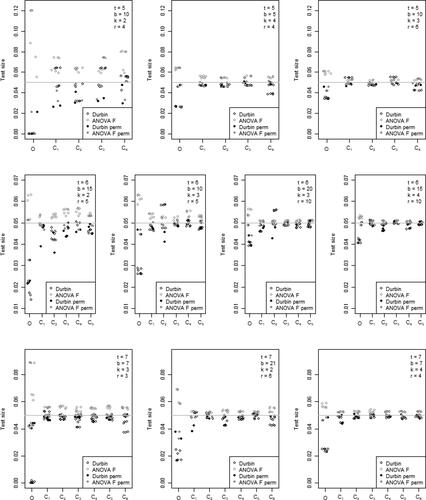
We now give results for the other BIBDs considered by Best and Rayner (2014). Sizes for tests using the ${\chi }^2$ and F distributions were calculated for all of the above distributions, however we only present those for U(0, 1) and DU(1, 3) in the following tables. Permutation test sizes were only calculated for U(0, 1) and DU(1, 3). Whilst the tables present results for these distributions, Figure 1 presents scatter plots of all test sizes calculated for designs with t = 5, 6, 7.

Figure 1. Scatter plots of all test sizes calculated for each design for t = 5, 6, 7. These are ordered from left to right based on observed adherence to the nominal significance level of 0.05.

Despite some differences in methodology, the test sizes calculated for the overall effects are roughly consistent with Best and Rayner (2014) for the following tables. In addition the test sizes for the overall effects are also consistent with those presented in Livingston Jr and Rayner (2022). With that in mind, we focus our commentary on the test sizes related to the contrast effects.

The design shown in Table 3 is a small design with a sample size of 12. The number of times data sets simulated resulted in an error mean square of zero was 19,792, 10,382, and 6,029 for DU(1, 3), DU(1, 5), and DU(1, 7) respectively out of 1,000,000 simulations. These proportions are not insignificant and might have inflated the contrast test sizes. The permutation test p-values do not appear to have appropriate test size, especially for DU(1, 3). The degree two test sizes for U(0, 1) using the ${\chi }^2$ and F distributions are too large.

For the design presented in Table 4, the contrasts appear to have test sizes reasonably close to 0.05. Here there were 504, 158, and 38 data sets created that resulted in error mean square equal to zero.

For the designs presented in Tables 5 and 6, the sample sizes are the same as the design in Table 4; however the contrasts all appear to have test sizes closer to 0.05. In both of these tables the F contrast sizes tend to be above 0.05 whereas the Durbin sizes tend to be below 0.05. The permutation sizes are all quite close to 0.05. The number of data sets with zero error mean square was 4 for the DU(0, 3) from the design in Table 5. There were no others.

Tables 7 to 10 all show test sizes for designs with t = 6. A similar observation can be made as for the earlier tables in that the test sizes are quite close to 0.05 and seem to improve as we move from Table 7 to 10. Also the Durbin and ANOVA F sizes appear to be less than and greater than 0.05 respectively most of the time.

The results in Tables 2, 11, and 12 are all for designs with t = 7. The same observation can be made for the designs with t = 7 as was made for the t = 6 designs. The test sizes are quite close to 0.05 and as we move from Table 2, to 11, to 12 the test sies appear to improve very slightly.

To visualize the observed changes in test sizes within designs with the same number of treatments, scatter plots of all test sizes calculated are presented in Figure 1. The first row of plots is for t = 5, followed by rows for t = 6 and t = 7. Each scatter plot shows Durbin test sizes in black and ANOVA test sizes in grey. The solid dots are for permutation tests and the hollow dots are for tests using the ${\chi }^2$ or F distributions. The scatter plots are ordered left to right in the same order as the tables are presented above and it appears that within a row of the plots, as kr increases, the test size appears to improve toward the nominal significance level of 0.05.

We now apply and compare the results with real world data.

4. Example

Breakfast Cereal Data. The data presented in Table 13 are from Kutner et al. (2005, Sec. 28.1) and are also analyzed in Rayner and Livingston Jr (2023a, sections 5.3 and 10.8). The design is a BIBD (3, 5, 6, 10) and the ANOVA F test on the ranks has p-value 0.0001.

Table 13. Rankings for breakfast cereals.

Judge	Cereal
	A	B	C	D	E
1	1.5	1.5	3
2	1	2.5		2.5
3	1.5	3			1.5
4	1		2	3
5	1.5		3		1.5
6	1			3	2
7		2	3	1
8		2.5	2.5		1
9		3		2	1
10			3	2	1
Sum	7.5	14.5	16.5	13.5	8

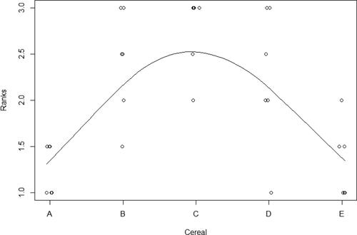
Rayner and Livingston Jr (2023a, 10.8) find a strong generalized correlation of degree (1, 2) (p-value less than 0.0001). Their analysis assumes treatments are ordered A < B < C < D < E, and suggests that as we pass from A to E the responses increase and then decrease. The mean ranks are 1.25, 2.42, 2.75, 2.25 and 1.33 respectively and a parabolic shape is evident in Figure 2. If the ordering is based on sugar content, then tasters preferred mid-range sugar content.

Figure 2. Mean ranks versus breakfast cereals.

Using the chi-squared sampling distributions the Durbin contrasts p-values are: $$0.0050,\text{1}.0000,0.0001,0.7055,\text{and}0.8864$$ for the overall effect, then contrast 1 to 4 respectively. Using the F sampling distributions, the corresponding ANOVA F p-values are: $$0.0000,\text{1}.000,0.0000,0.5145,\text{and}0.8043,$$ respectively. The simulation study for this design suggested that the test sizes using the ${\chi }^2$ or F distributions had good adherence to the nominal significance level of 0.05. The permutation tests were significantly better though in terms of root mean square error.

Using 100,000 permutations the Durbin p-values are: $$0.0006,0.9827,0.0000,0.7103,\text{and}0.9455,$$ and the ANOVA F p-values are: $$0.0006,0.9815,0.0001,0.5100,\text{and}0.8372,$$ for the overall effect, followed by contrasts 1 to 4. These calculations were performed using the CMHNPA package (Livingston Jr and Rayner 2023) in R (R Core Team 2023).

The overall Durbin and ANOVA F tests are significant at the 0.01 level: there is strong evidence of a difference in the treatment mean ranks. The contrast p-values indicate that there is strong quadratic at the 0.001 level. This is the only contrast effect that is present.

5. Conclusion

The ability to formally analyze higher order effects in ordered treatments in the BIBD is an insightful instrument for data analysts’ tool kits. To do so effectively, designs with small sample sizes (bk) should be avoided and within a particular number of treatments, a larger kr appears to improve test sizes.

For testing overall effects, we confirm the superiority of the ANOVA F test on the ranks over the Durbin test. For testing the contrasts, the Durbin contrasts have a very slight advantage over the ANOVA F, however this was not constant across all the designs. If one is using the ANOVA F for the overall effects, it would be acceptable to therefore use the corresponding contrasts.

Ultimately however, the permutation tests using either the Durbin or ANOVA F tests are preferred. For the overall effects they are the same test due to the one-to-one relationship between the test statistics. For the contrasts, both resulted in similar root mean square errors with neither superior to the other across the different designs. Therefore either is acceptable.

Given that the ANOVA F test outperforms the Durbin test for the overall effect, it was expected that this would carry over into the contrast tests. It was surprising to find that this was not the case. Another surprising result was that the contrast test sizes are reasonably close to the nominal 0.05 in some of the smaller designs, even when the overall effect has unsatisfactory sizes.

It is appropriate to conclude with a brief reference to the place of contrasts in inference. It is tempting for data analysts to apply a test such as the Durbin, and if it proves to be significant, and only then, to investigate the failure of the null hypothesis by calculating contrasts. Two problems with this approach are.

• First, frequently the more omnibus Durbin test may not be significant when at least one of the more directional contrasts is. Thus not investigating the contrasts may mean an important effect is missed.

• The second issue is that formal inference is clouded by using the Durbin as a pretest. Rejection of the null hypothesis is conditional on first, the rejection of the pretest, and then on the rejection based on at least one of the contrasts. Thus allowance must be made for both pretesting and applying multiple (contrast) tests. Additionally there is the issue of exactly what the null hypothesis is.

Our approach is that we would normally use the Durbin test formally and then investigate the contrasts in much the same way as providing an informal plot of treatment mean ranks against treatments: as exploratory data analysis. An alternative is to immediately formally test for significance using the first three or four contrasts and adjust for performing multiple tests.

In the breakfast cereals example p-values are given for both the Durbin and ANOVA F tests on the ranks to show the application of both. In practice we would use just one, usually the latter, and calculate the contrasts in an exploratory data analytic manner.

Disclosure statement

No potential conflict of interest was reported by the author(s).

References

- Best, D. J., and J. C. W. Rayner. 2014. Conover’s F test as an alternative to Durbin’s test. Journal of Modern Applied Statistical Methods 13 (2):76–83. doi: 10.22237/jmasm/1414814580.
- Kutner, M., C. Nachtsheim, J. Neter, and W. Li. 2005. Applied linear statistical models (5th ed.). Boston: McGraw-Hill Irwin.
- Lancaster, HO. 1965. The Helmert matrices. The American Mathematical Monthly 72 (1):4–12. doi: 10.1080/00029890.1965.11970483.
- Livingston Jr, G. C., and J. C. W. Rayner. 2022. Non-parametric analysis of balanced incomplete block rank data. Journal of Statistical Theory and Practice 16 (4):66. doi: 10.1007/s42519-022-00287-3.
- Livingston Jr, G. C., and J. C. W. Rayner. 2023. CMHNPA: Cochran-Mantel-Haenszel and Nonparametric ANOVA. R package version 1.1.1, https://CRAN.R-project.org/package=CMHNPA.
- R Core Team. 2023. R: A language and environment for statistical computing. R Foundation for Statistical Computing, Vienna, Austria. https://www.R-project.org/.
- Rayner, J. C. W, and G. C. Livingston Jr. 2023a. An introduction to Cochran–Mantel–Haenszel testing and nonparametric ANOVA. Chichester: Wiley.
- Rayner, J. C. W, and G. C. Livingston Jr. 2023b. ANOVA F orthonormal contrasts for ordered treatments in multifactor fixed effects ANOVAs. Submitted.
- Rayner, J. C. W, and G. C. Livingston Jr. 2023c. Orthogonal contrasts for both balanced and unbalanced designs and both ordered and unordered treatments. Statistica Neerlandica 78 (1):68–78. doi: 10.1111/stan.12305.
- Rayner, J. C. W., O. Thas, and B. De Boeck. 2008. A generalised Emerson recurrence relation. Australian & New Zealand Journal of Statistics 50 (3):235–40. doi: 10.1111/j.1467-842X.2008.00514.x.
- Thas, O., D. J. Best, and J. C. W. Rayner. 2012. Using orthogonal trend contrasts for testing ranked data with ordered alternatives. Statistica Neerlandica 66 (4):452–71. doi: 10.1111/j.1467-9574.2012.00525.x.