On the effect of the Kaplan-Meier estimator’s assumed tail behavior on goodness-of-fit testing

Abstract

When analyzing lifetime data in the presence of censoring one is often required to estimate the distribution function of the lifetimes non-parametrically. The most popular estimator used for this purpose is the Kaplan-Meier estimator. Interestingly, in its initial formulation this estimator is only defined up to the observed sample maximum. For values larger than the sample maximum two different assumptions are commonly used in the statistical literature. The first is to set the value of the estimate to one while the second is to use the value of the estimate at the sample maximum when estimating the tail of the distribution function. This paper illustrates the profound effect of these assumptions on the sizes and powers of goodness-of-fit tests for three classes of distributions often used in survival analysis. These differences are illustrated using observed remission time data. The considered classes of distributions are the exponential, Weibull and gamma. As a result of independent interest, we amend two classes of tests developed for the gamma distribution in the full sample case for use with censored data.

Keywords:

• Exponential distribution
• Gamma distribution
• Goodness-of-fit testing
• Kaplan-Meier estimate
• Random right censoring
• Weibull distribution

1. Introduction

Statistical practitioners and other researchers are often interested in the parametric modeling of observed lifetime data in survival analysis, reliability theory as well as many other fields. In order to perform inference, it is necessary to test the goodness-of-fit hypothesis that the observed lifetimes are realized from a specified class of distributions. This hypothesis is complicated by the fact that random right censoring is often present in the applications of interest. Testing the goodness-of-fit of a specific class of distributions is a topic of continued interest; recent papers on this topic include (Cuparić and Milošević 2021) and (Bothma et al. 2021) (in which the assumption of exponentiality is tested) as well as (Kim 2017) (in which the assumption of the class of Weibull distributions is tested).

In the full sample case, the classical goodness-of-fit tests are based on comparisons between non-parametric and parametric estimates of the distribution function (obtained by estimating the parameters of the specified class of distributions under the null hypothesis). Consider, for example, the Cramér-von Mises test, see D’Agostino and Stephens (1986). The idea underlying this test is to compare the empirical distribution function to a fitted parametric distribution function obtained by estimating the parameters (using consistent estimators) of the specified class of distributions. If the distance between the two estimates, as measured by an integral involving the squared difference between the empirical distribution function and the fitted distribution, is “too large” (to be made precise below), then the null hypothesis is rejected. In fact, this approach also underlies other classical goodness-of-fit tests such as the Kolmogorov-Smirnov test, which is obtained upon replacing the distance measure above by the supremum difference.

A natural approach to the goodness-of-fit problem in the presence of censoring is to extend the techniques described above to account for censoring. That is, in the presence of censoring, the Cramér-von Mises test for a class of distributions is based on a specified distance between a non-parametric estimate of the distribution function, similar to the empirical distribution function, and a parametric estimate of the distribution function under the null hypothesis. Parameter estimation in the presence of random right censoring has been studied extensively in the literature, see e.g. Cox and Oakes (1984) as well as Datta (2005). The most popular estimation technique used is the method of maximum likelihood; this method is used for parameter estimation throughout this paper. It remains to find a non-parametric estimate of the distribution function. This can be achieved using the well-known Kaplan-Meier estimator, see Kaplan and Meier (1958). In order to proceed we introduce some notation below.

Let $X_1,\dots ,X_n$ denote independent and identically distributed (i.i.d.) lifetimes with continuous distribution and density functions F and f, respectively. Let $C_1,\dots ,C_n$ be i.i.d. censoring variables with continuous distribution function G, independent of $X_1,\dots ,X_n.$ We assume that the censoring mechanism used is non-informative. The observed times are $T_j=\mathrm{\text{min}}(X_j,C_j),j=1,\dots ,n,$ and we define the indicator variables ${\delta }_j=\mathrm{I}(X_j\le C_j).$ The order statistics of T_j are denoted $T_{(1)}\le \dots \le T_{(n)},$ with ${\delta }_{(j)}$ corresponding to $T_{(j)}.$ Let ${\mathcal{F}}_{\theta }$ denote a parametric class of distribution functions indexed by some, possibly vector valued, parameter θ. Based on the observed pairs $(T_j,{\delta }_j),j=1,\dots ,n$ we wish to test the composite goodness-of-fit hypothesis $$H_0:F\in {\mathcal{F}}_{\theta },$$ against general alternatives. In this paper, we present numerical results relating to three classes of distributions, the exponential, Weibull and gamma. References to recent papers relating to testing for the first two of these are provided above. However, we have been unable to obtain any papers relating to goodness-of-fit testing for the gamma distribution in the presence of censoring. In Sec. 2, we adapt several existing tests for the gamma distribution in the full sample case for use with random right censored data.

Using the notation introduced above, the Kaplan-Meier estimator, ${\tilde{F}}_n,$ is a step function given by (1) $${\tilde{F}}_n(t)=\{\begin{array}{ll}0,\hfill & 0<t\le T_{(1)},\hfill \\ 1-\prod _{j=1}^{k-1}{\left(\frac{n-j}{n-j+1}\right)}^{{\delta }_{(j)}},\hfill & T_{(k-1)}<t\le T_{(k)},k=2,\dots ,n.\hfill \end{array}$$(1)

Interestingly, in its initial formulation, the Kaplan-Meier estimator of the distribution function is only defined up to the sample maximum, say $\tau =T_{(n)}.$ In cases where the maximum observation is censored, two different assumptions or conventions are commonly used in the statistical literature to define ${\tilde{F}}_n(t)$ for $t>\tau .$ The first is to simply set the value of ${\tilde{F}}_n(t)=1,\forall t>\tau ,$ see e.g. Efron (1981), while the second is to set ${\tilde{F}}_n(t)={\tilde{F}}_n(\tau ),\forall t>\tau ,$ see e.g. Cox and Oakes (1984). For the sake of brevity, we refer to this convention as the “set-to-1” convention; i.e. we refer to the first and second conventions mentioned above as cases where the set-to-1 assumption is made and not made, respectively.

Regardless of the set-to-1 assumption, all jumps in ${\tilde{F}}_n$ occurring before the sample maximum occur at values of T_j for which ${\delta }_j=1.$ If the sample maximum τ is uncensored, then the final jump in ${\tilde{F}}_n$ occurs at τ regardless of the set-to-1 assumption. However, if the sample maximum is censored, then the set-to-1 assumption influences the tail behavior of ${\tilde{F}}_n,$ i.e. the value of ${\tilde{F}}_n(t),t>\tau .$ If the set-to-1 assumption is made the final jump occurs immediately after τ; however, if this assumption is not made there is no jump immediately following τ. The latter case results in an improper distribution with positive probability of realizing the value $\infty .$ In summary, the set-to-1 assumption only influences the estimate ${\tilde{F}}_n$ if the sample maximum is censored, and then it only affects ${\tilde{F}}_n(t),t>\tau .$ This paper illustrates the profound effect that this seemingly small difference has on the powers of goodness-of-fit tests by conducting an extensive Monte Carlo simulation study. Before we proceed, the effect of the assumption used in the Kaplan-Meier estimator is demonstrated using an example based on observed data below.

A data set containing 66 initial remission times of leukemia patients, 14 of which are censored, is presented in (Lee and Wang 2003). The data are shown in Table 1, censored observations are indicated using an asterisk in the superscript. Initially, the data were segmented into three groups based on the treatments that the patients received. However, (Lee and Wang 2003) found no statistically significant differences between the groups, so we treat the data as realizations from a single distribution. Figure 1 shows the Kaplan-Meier estimate of the distribution function using both of the assumptions discussed above. The two Kaplan-Meier step functions considered coincide up to the sample maximum value of 269 (indicated in Figure 1 using a dotted vertical line). However, since the last observation is censored, the two versions of this estimate differ when t > 269. Under the set-to-1 assumption, ${\tilde{F}}_n(t)=1,\forall t>269.$ If this assumption is not made, then ${\tilde{F}}_n(t)=0.853,\forall t>269.$ As can be seen in the figure, the set-to-1 assumption makes a substantial difference in the estimated value of the distribution function for large values of t. Additionally, Figure 1 shows two parametric estimates of the distribution function obtained using exponential and Weibull distributions, respectively. The techniques used to obtain these parametric estimates are discussed.

Figure 1. Kaplan-Meier Estimate of the lifetimes with fitted exponential and Weibull distributions.

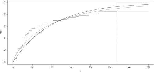
Table 1. Initial remission times of leukemia patients in days.

$4,5,8,8,9,10,10,10,10,10,11,12,12,{12}^{*},13,14,20,{20}^{*},23,23,25,25,25,28,28,28,$

$28,29,31,31,31,32,37,40,41,41,48,48,57,62,70,74,75,89,99,100,103,124,139,143,$

${159}^{*},{161}^{*},162,169,{190}^{*},195,{196}^{*},{197}^{*},{199}^{*},{205}^{*},{217}^{*},{219}^{*},220,{245}^{*},{258}^{*},{269}^{*}$

As a first parametric model, consider the class of exponential distributions, with density $f(t)=\lambda {\mathrm{e}}^{-\lambda t},\lambda >0,t>0.$ We denote a random variable having this density by $\mathrm{\text{exp}}(\lambda ).$ The maximum likelihood estimate of the rate parameter of the exponential distribution is $$\widehat{\lambda }=\frac{{\sum }_{j=1}^n{\delta }_j}{{\sum }_{j=1}^n{T}_j}.$$

For the example at hand, $\widehat{\lambda }=0.01.$ Figure 1 shows the fitted exponential distribution function using a solid line. Additionally, we fit a Weibull distribution to the observed data. The density of the Weibull distribution with parameters κ and λ is $f(t)=\kappa {\lambda }^{\kappa }{t}^{\kappa -1}{\mathrm{e}}^{-{(\lambda t)}^{\kappa }},\kappa >0,\lambda >0,t>0$. A random variable with this density is denoted by $W(\kappa ,\lambda ).$ The log-likelihood of the $W(\kappa ,\lambda )$ distribution, given $(T_j,{\delta }_j),j=1,\dots ,n,$ is $$\mathcal{L}(\kappa ,\lambda |X_1,\dots ,X_n)=d\hspace{0.17em}\mathrm{\text{log}}\hspace{0.17em}(\kappa )+d\kappa \hspace{0.17em}\mathrm{\text{log}}\hspace{0.17em}(\lambda )+(\kappa -1)\sum _{j=1}^n{\delta }_j\hspace{0.17em}\mathrm{\text{log}}\hspace{0.17em}(X_j)-{\lambda }^{\kappa }\sum _{j=1}^n{X}_j^{\kappa },$$ where $d={\sum }_{j=1}^n{\delta }_j.$ Closed form formulae for the maximum likelihood estimators of κ and λ are not available. The required estimates are obtained using numerical optimization. All calculations presented are performed in R, see R Core Team (2019). We estimate the parameters of the Weibull distribution using the $\mathit{\text{fit}}\_\mathit{\text{data}}$ function in the parmsurvfit package, see Jacobson, Wilson, and Pileggi (2018). For the current example, the parameter estimates obtained are $\widehat{\kappa }=0.812$ and $\widehat{\lambda }=0.01.$ The fitted Weibull distribution function is shown in Figure 1 using a dotted line.

Figure 1 provides us with a visual test of fit for both the exponential and Weibull distributions; the fitted Weibull seems to resemble the non-parametric estimates more closely than does the fitted exponential. This is to be expected as the exponential distribution is a special case of the Weibull. In order to formally test the goodness-of-fit hypotheses of interest, we use the Cramér-von Mises test for both classes of distributions in turn. Goodness-of-fit test statistics for the exponential and Weibull distributions are typically performed based on transformed data. In the case of the exponential distribution, we rescale the data by multiplication with the estimated rate parameter. This essentially reduces the null hypothesis to testing for standard exponentiality. In the same way, we may use a transformation to reduce the test for the Weibull class of distributions to a test for the standard extreme value distribution; i.e. $X\sim W(\kappa ,\lambda )$ if, and only if, $Y=\lambda (\hspace{0.17em}\mathrm{\text{log}}\hspace{0.17em}(X)-\hspace{0.17em}\mathrm{\text{log}}\hspace{0.17em}(\kappa ))$ follows a standard extreme value distribution. That is, Y has density $h(x)={\mathrm{e}}^{x-{\mathrm{e}}^x},x\in \mathbb{R}.$ We denote the variables resulting from the sample version of this transformation by $Y_j=\widehat{\lambda }\left[\mathrm{\text{log}}\hspace{0.17em}(T_j)-\hspace{0.17em}\mathrm{\text{log}}\hspace{0.17em}(\widehat{\kappa })\right],j=1,\dots ,n,$ for both the exponential and Weibull classes (as well as for the gamma class later in the paper). Using transformations of this kind is standard practice in the goodness-of-fit literature, see e.g. Allison et al. (2017) and Bothma, Allison, and Visagie (2022) as well as Henze and Visagie (2020). Below, we use $F_{\widehat{\theta }}$ and ${\tilde{F}}_n$ to denote the fitted distribution function and the Kaplan-Meier estimate of the distribution function, respectively.

Let CM_n denote the Cramér-von Mises test statistic based on $(Y_j,{\delta }_j),j=1,\dots ,n.$ As was mentioned above, CM_n is a distance measure between the parametric estimate $F_{\widehat{\theta }}$ and the non-parametric estimate ${\tilde{F}}_n;$ (2) $$C{M}_n={\int }_{-\infty }^{\infty }{(F_{\widehat{\theta }}(t)-{\tilde{F}}_n(t))}^2\mathrm{d}{F}_{\widehat{\theta }}(t).$$(2)

We can exploit the fact that ${\tilde{F}}_n$ is a step function in order to arrive at an easily calculable expression for CM_n. Using notation similar to that of (D’Agostino and Stephens 1986), denote by $y_j,j=1,\dots ,d,$ the set of uncensored lifetimes and let $\tilde{\tau }$ be the transformed value of the sample maximum. The Cramér-von Mises test statistic defined in (2)(2) $$C{M}_n={\int }_{-\infty }^{\infty }{(F_{\widehat{\theta }}(t)-{\tilde{F}}_n(t))}^2\mathrm{d}{F}_{\widehat{\theta }}(t).$$(2) can be expressed as $$\begin{array}{l}C{M}_n=\frac{n}{3}+n\sum _{j=1}^d{\tilde{F}}_n(y_{j-1})\left[F_{\widehat{\theta }}(y_j)-F_{\widehat{\theta }}(y_{j-1})\right]\left[{\tilde{F}}_n(y_{j-1})-\left(F_{\widehat{\theta }}(y_j)-F_{\widehat{\theta }}(y_{j-1})\right)\right]\\ +n{\tilde{F}}_n(y_d)\left[F_{\widehat{\theta }}(\tilde{\tau })-F_{\widehat{\theta }}(y_d)\right]\left[{\tilde{F}}_n(y_d)-\left(F_{\widehat{\theta }}(\tilde{\tau })-F_{\widehat{\theta }}(y_d)\right)\right]\\ +n{\tilde{F}}_n^{+}(\tilde{\tau })\left[1-F_{\widehat{\theta }}(\tilde{\tau })\right]\left[{\tilde{F}}_n^{+}(\tilde{\tau })-\left(1-F_{\widehat{\theta }}(\tilde{\tau })\right)\right],\end{array}$$ where $g^{+}(t)$ denotes the right limit of the function g. In the case where the set-to-1 assumption is made, the formula above coincides with the formula given in (D’Agostino and Stephens 1986).

For the example under consideration, the sample maximum is censored, meaning that the calculated value of ${\tilde{F}}_n,$ and therefore the value of CM_n, depends on the set-to-1 assumption. Consider first the case where ${\mathcal{F}}_{\theta }$ is the class of exponential distributions. When making the set-to-1 assumption, CM_n is calculated to be 0.543. If this assumption is not made, then CM_n equals 0.596.

In order to formally test the hypothesis that the lifetimes are realized from an exponential distribution, we need to approximate the distribution of the test statistic under the null hypothesis. In the full sample case, the fact that the exponential class of distributions is a scale family ensures that the distribution of the CM_n under the null hypothesis is independent of the value of λ. However, in the setup considered in this paper, we are unable to exploit this feature of the exponential class as even the hypothesis that lifetimes are standard exponential is a composite hypothesis since the censoring distribution remains unspecified. As a result, we use a bootstrap algorithm in order to approximate the null distribution of CM_n. Appropriate bootstrap algorithms for use with the exponential and Weibull classes can be found in (Bothma et al. 2021) and (Bothma, Allison, and Visagie 2022), respectively. However, the provided algorithms specifically assume that the set-to-1 convention is not used. Below we provide a more general algorithm in which the user can specify whether or not to make the set-to-1 assumption.

In order to proceed, we need to be able to obtain bootstrap samples from both the lifetime and censoring distributions. Generating samples from the lifetime distribution under the null hypothesis is a simple matter; we estimate the parameters of the specified class of distributions and we simulate from this fitted distribution (using, e.g. the inverse transform method). Since the null hypothesis does not specify the censoring distribution, we need to estimate this distribution from the observed data. We use the Kaplan-Meier estimator of the distribution of the censored observations; this is done by calculating ${\tilde{F}}_n$ in (1)(1) $${\tilde{F}}_n(t)=\{\begin{array}{ll}0,\hfill & 0<t\le T_{(1)},\hfill \\ 1-\prod _{j=1}^{k-1}{\left(\frac{n-j}{n-j+1}\right)}^{{\delta }_{(j)}},\hfill & T_{(k-1)}<t\le T_{(k)},k=2,\dots ,n.\hfill \end{array}$$(1) , but replacing δ_j by $1-{\delta }_j$ in the calculations. Of course, since we are using the Kaplan-Meier estimator to estimate the distribution of the censoring times, we are confronted with the set-to-1 assumption once again. Immediately, one is tempted to argue that whatever convention was used to estimate the distribution function of the lifetimes should be used in order to estimate the distribution function of the censoring times. However, there is no contradiction in, e.g. making the set-to-1 assumption for the censoring times and not for the lifetimes. In order to ease notation in the remainder of the paper we use the notation “TF” in order to indicate this specific combination of conventions since it means that we assume that the set-to-1 assumption is “true” for the censoring distribution and “false” for the lifetime distribution. As a result, we are left with four distinct possibilities:

• Case 1: The set-to-1 assumption is not made for either of the estimated distributions (indicated by “FF”).

• Case 2: The set-to-1 assumption is made for the lifetime distribution but not for the censoring distribution (indicated by “FT”).

• Case 3: The set-to-1 assumption is made for the censoring distribution but not for the lifetime distribution (indicated by “TF”).

• Case 4: The set-to-1 assumption is made for both of the estimated distributions (indicated by “TT”).

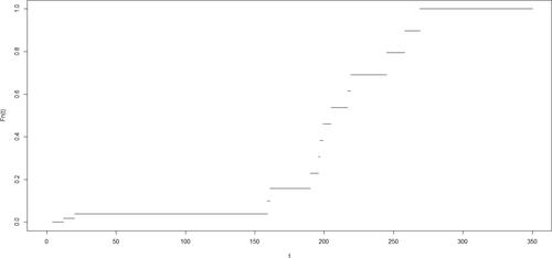
The Kaplan-Meier estimate of the censoring distribution in the practical example is shown in Figure 2. Since the sample maximum is censored, the Kaplan-Meier estimate achieves the value of 1 at t = 269 regardless of the set-to-1 assumption.

Figure 2. Kaplan-Meier Estimate of the censored remission times.

We now provide the bootstrap algorithm required in order to approximate critical values for goodness-of-fit tests in the presence of random right censoring.

1. Using $(T_j,{\delta }_j),j=1,\dots ,n,$ estimate the parameters of the class of distributions as specified in H₀.

2. Obtain a parametric bootstrap sample $X_1^{*},\dots ,X_n^{*}$ by sampling from the fitted distribution.

3. Obtain a non-parametric bootstrap sample $C_1^{*},\dots ,C_n^{*}$ by sampling from the Kaplan-Meier estimate of the distribution of the censoring times (setting the set-to-1 assumption to true or false).

4. Set $$T_j^{*}=\mathrm{\text{min}}(X_j^{*},C_j^{*})\text{and}{\delta }_j^{*}=\{\begin{array}{cc}1,\hfill & \text{if}{X}_j^{*}\le C_j^{*}\hfill \\ 0,\hfill & \text{if}{X}_j^{*}>C_j^{*}.\hfill \end{array}$$

5. Using $(T_j^{*},{\delta }_j^{*})$ estimate the parameters of the class of distributions and use the transformation to obtain $Y_j^{*},j=1,\dots ,n.$

6. Based on the data $(Y_j^{*},{\delta }_j^{*}),j=1,\dots ,n,$ calculate the value of the test statistic, say $S^{*}=S((Y_1^{*},{\delta }_1^{*}),\dots ,(Y_n^{*},{\delta }_n^{*})).$

7. Repeat steps 2-6 B times, resulting in $S_1^{*},\dots ,S_B^{*}.$ Denote the corresponding order statistics by $S_{(1)}^{*}\le \dots \le S_{(B)}^{*}.$ The approximate critical value is ${\widehat{c}}_n(\alpha )=S_{(\lfloor B(1-\alpha )\rfloor )}^{*}$ where $\lfloor ·\rfloor$ denotes the floor function.

The algorithm presented above is general and not only intended for use with the exponential null hypothesis. Using this algorithm, and setting $B=50 000,$ we obtain an approximation to the null distribution of the CM_n statistic when testing for the exponential class. In the current example, the set-to-1 assumption regarding the Kaplan-Meier estimate of the censoring distribution is unimportant since it does not influence the resulting estimated distribution function. However, the set-to-1 convention used influences the value of the test statistic obtained and therefore the p-value of the test. In this case, an approximate p-value of 0.00072 is obtained when making the set-to-1 assumption, while the p-value is estimated to be 0.00032 when not using this assumption. In both cases, we reject the hypothesis that the lifetimes are realized from an exponential distribution at a significance level of 1%.

We now turn our attention to the hypothesis that the lifetimes are realized from the Weibull class of distributions. The value of CM_n is calculated to be 0.244 when making the set-to-1 assumption, which corresponds to a p-value of 0.019. If this assumption is not made, the calculated value of CM_n is 0.290, corresponding to a p-value of 0.011. As a result, we do not reject the hypothesis that the lifetimes follow a Weibull distribution at a 1% significance level.

The final class of distributions considered is the gamma class. A random variable with density $f(t)={\lambda }^{\kappa }{\Lambda }^{-1}(\kappa )t^{\kappa -1}{\mathrm{e}}^{-\lambda t},\kappa >0,\lambda >0,t>0,$ with $\Lambda (\kappa )={\int }_0^{\infty }{x}^{\kappa -1}{\mathrm{e}}^{-x}\mathrm{d}x,$ is said to have a gamma distribution with shape parameter κ and rate parameter λ. We denote a random variable with this density by $\Gamma (\kappa ,\lambda ).$ When testing the hypothesis that the remission times considered are realized from a gamma distribution, we calculate CM_n to be 0.376 and 0.326 respectively when making the set-to-1 assumption and not making this assumption. In both cases, the corresponding p-value is below 1%, meaning that we reject the class of gamma distributions as a suitable model for the lifetimes.

2. Test statistics for the various classes of lifetime distributions

Below, we provide the details of a number of goodness-of-fit tests for the exponential, Weibull and gamma classes. The performances of the tests in this section are evaluated in a Monte Carlo simulation study presented in Sec. 3. We begin by specifying the classical Kolmogorov-Smirnov test. As is the case for the Cramér-von Mises test, discussed in Sec. 1, the Kolmogorov-Smirnov test is general in the sense that it can be used to test for any of the classes of distributions mentioned above.

After considering the Kolmogorov-Smirnov test, we turn our attention to tests developed for each of the considered classes of distributions separately. The remaining tests are based on the characteristic function and Laplace transform. These functions and their empirical counterparts have been studied extensively in the full sample case, see e.g. Meintanis (2016). However, estimates for the empirical versions of these functions are less well known in the presence of censoring. As a result, we discuss these functions before defining the relevant test statistics.

2.1. The Kolmogorov-Smirnov test

The Kolmogorov-Smirnov (KS_n) test measures the supremum distance between ${\tilde{F}}_n$ and $F_{\widehat{\theta }};$ $$K{S}_n={\text{sup}}_{t>0}|F_{\widehat{\theta }}(t)-{\tilde{F}}_n(t)|.$$

Similar to the full sample case, the differences need only be evaluated in the jump points of the piecewise constant ${\tilde{F}}_n.$ The value of KS_n can be calculated as (3) $$K{S}_n=\mathrm{\text{max}}\{K{S}_n^{+},K{S}_n^{-},1-{\mathrm{\text{lim}}}_{t\to \infty }{\tilde{F}}_n(t)\},$$(3) where $$K{S}_n^{+}=\underset{1\le j\le n}{\mathrm{\text{max}}}\left\{{\tilde{F}}_n(Y_{(j)})-F_{\widehat{\theta }}(Y_{(j)})\right\}$$ and $$K{S}_n^{-}=\underset{1\le j\le n}{\mathrm{\text{max}}}\left\{F_{\widehat{\theta }}(Y_{(j)})-{\tilde{F}}_n(Y_{(j-1)})\right\},$$ with $Y_{(0)}:=0.$ Note that, if the set-to-1 assumption is made, then ${\mathrm{\text{lim}}}_{t\to \infty }{\tilde{F}}_n(t)=1$ for all samples and the final term in (3)(3) $$K{S}_n=\mathrm{\text{max}}\{K{S}_n^{+},K{S}_n^{-},1-{\mathrm{\text{lim}}}_{t\to \infty }{\tilde{F}}_n(t)\},$$(3) can be omitted.

2.2. Empirical characteristic function and Laplace transforms

Recall that the characteristic function of a random variable, Y, with distribution function, F, is defined to be $$\varphi (s)=\mathrm{E}\left[{\mathrm{e}}^{\mathit{\text{isY}}}\right]=\int {\mathrm{e}}^{\mathit{\text{isy}}}\mathrm{d}F(y),$$ with $i=\sqrt{-1}.$ Using the notation introduced above and using ${\tilde{F}}_n$ to estimate F, we may estimate the characteristic function based on a censored sample by $${\tilde{\varphi }}_n(s)=\int {\mathrm{e}}^{\mathit{\text{isy}}}\mathrm{d}{\tilde{F}}_n(y)=\sum _{j=1}^n{\Delta }_j{\mathrm{e}}^{\mathit{\text{is}}{Y}_{(j)}},$$ see e.g. Csörgö (1984), where Δ_j denotes the size of the jump in ${\tilde{F}}_n(Y_{(j)}),j=1,\dots ,n,$ given by $${\Delta }_1=\frac{{\delta }_{(1)}}{n},{\Delta }_n=\prod _{l=1}^{n-1}{\left(\frac{n-l}{n-l+1}\right)}^{{\delta }_{(l)}},{\Delta }_j=\frac{{\delta }_{(j)}}{n-j+1}\prod _{k=1}^{j-1}{\left(\frac{n-k}{n-k+1}\right)}^{{\delta }_{(k)}},j=2,\dots ,n-1.$$

Additionally, recall that the Laplace transform of a random variable Y is defined as $$\psi (s)=\int {\mathrm{e}}^{-\mathit{\text{sy}}}\mathrm{d}F(y).$$

Upon estimating F by ${\tilde{F}}_n,$ the resulting estimate of the Laplace transform is $${\tilde{\psi }}_n(s)=\sum _{j=1}^n{\Delta }_j{\mathrm{e}}^{-s{Y}_{(j)}}.$$

2.3. Tests for the exponential distribution

We now consider four tests for the exponential distribution in the presence of random right censoring. The first two tests are based on the empirical characteristic function while the last two are based on the empirical Laplace transform. Three of the tests below contains a user defined tuning parameter a > 0.

2.3.1. Henze-Meintanis (2002a)

A test statistic based on a characterization of the exponential distribution via the characteristic function is introduced in Henze and Meintanis (2002a). In the presence of random censoring, the modified test is given by $$H_{n,a}=n{\int }_0^{\infty }{\left[S_n(t)-t{C}_n(t)\right]}^2{\mathrm{e}}^{-\mathit{\text{at}}}\mathrm{d}t,$$ where $S_n(t)={\sum }_{j=1}^n{\Delta }_j\hspace{0.17em}\mathrm{\text{sin}}\hspace{0.17em}(t{Y}_j)$ and $C_n(t)={\sum }_{j=1}^n{\Delta }_j\hspace{0.17em}\mathrm{\text{cos}}\hspace{0.17em}(t{Y}_j).$ An easily computable form of the test statistic is $$\begin{array}{l}{H}_{n,a}=\frac{\mathit{\text{an}}}{2}\sum _{j=1}^n\sum _{k=1}^n{\Delta }_j{\Delta }_k[\frac{1}{a^2+{\left(Y_j-Y_k\right)}^2}-\frac{1}{a^2+{\left(Y_j+Y_k\right)}^2}-\frac{4\left(Y_j+Y_k\right)}{{\left(a^2+{\left(Y_j+Y_k\right)}^2\right)}^2}\\ +\frac{2a^2-6{\left(Y_j-Y_k\right)}^2}{{\left(a^2+{\left(Y_j-Y_k\right)}^2\right)}^3}+\frac{2a^2-6{\left(Y_j+Y_k\right)}^2}{{\left(a^2+{\left(Y_j+Y_k\right)}^2\right)}^3}].\end{array}$$

In the simulation study in Sec. 3, we set a = 1 in accordance with the recommendation made in Henze and Meintanis (2002a). The null hypothesis of exponentiality is rejected for large values of $H_{n,a}.$

2.3.2. Baringhaus-Henze (1991)

Baringhaus and Henze (1991) introduces a test statistic based on a partial differential equation involving the Laplace transform. In the presence of random censoring the test statistic becomes $$B_{n,a}=n{\int }_0^{\infty }{\left[(1+t){\tilde{\psi }}_n^{\prime }(t)+{\tilde{\psi }}_n(t)\right]}^2{\mathrm{e}}^{-\mathit{\text{at}}}\mathrm{d}t,$$ where ${\tilde{\psi }}_n^{\prime }$ is the derivative of ${\tilde{\psi }}_n.$ The calculable form of the modified test is given by $$B_{n,a}=n\sum _{j=1}^n\sum _{k=1}^n{\Delta }_j{\Delta }_k\left[\frac{(1-Y_j)(1-Y_k)}{Y_j+Y_k+a}-\frac{Y_j+Y_k}{{(Y_j+Y_k+a)}^2}+\frac{2Y_j{Y}_k}{{(Y_j+Y_k+a)}^2}+\frac{2Y_j{Y}_k}{{(Y_j+Y_k+a)}^3}\right].$$

In the simulation study below we use a = 0.25. The null hypothesis of exponentiality is rejected for large values of $B_{n,a}.$

2.3.3. Henze-Meintanis (2002b)

A test statistic based on the squared difference between the Laplace transform and its empirical counterpart is proposed in Henze and Meintanis (2002b). In the presence of censoring, the modified test can be expressed as $$L_{n,a}=n{\int }_0^{\infty }{\left[{\tilde{\psi }}_n(t)-\psi (t)\right]}^2{(1+t)}^2{\mathrm{e}}^{-\mathit{\text{at}}}\mathrm{d}t.$$

This test statistic lends itself to the following easily calculable form; $$L_{n,a}=n\sum _{j=1}^n\sum _{k=1}^n{\Delta }_j{\Delta }_k\left[\frac{1+{(Y_j+Y_k+a+1)}^2}{{(Y_j+Y_k+a)}^3}\right]-2n\sum _{j=1}^n{\Delta }_j\left[\frac{1+Y_j+a}{{(Y_j+a)}^2}\right]+\frac{n}{a}.$$

We obtain the results in the simulation study by setting a = 0.25 as is recommended in (Henze and Meintanis 2002b). The null hypothesis is rejected for large values of $L_{n,a}.$

2.4. Tests for the Weibull distribution

Below we consider three tests for the Weibull distribution in the presence of random right censoring. The first two tests are based on Stein’s method for the approximation of integrals while the final test is based on the Laplace transform of the standard extreme value distribution.

2.4.1. Bothma-Allison-Visagie (2021)

Bothma, Allison, and Visagie (2022) proposes new classes of tests for the Weibull distribution based on Stein’s method. This test statistic is defined as (4) $$S_{n,a}=n{\int }_{-\infty }^{\infty }{\left|\sum _{j=1}^n{\Delta }_j[\mathit{\text{it}}{\mathrm{e}}^{\mathit{\text{it}}{Y}_j}+(1-{\mathrm{e}}^{Y_j}){\mathrm{e}}^{\mathit{\text{it}}{Y}_j}]\right|}^2{w}_a(t)\mathrm{d}t,$$(4) where $w_a(t)$ is a weight function containing a user-defined tuning parameter a > 0. The use of two weight functions resulted in two different classes of test statistics. For the first weight function, ${\mathrm{e}}^{-a{t}^2},$ the test statistic is given by $$\begin{array}{c}{S}_{n,a}^{(1)}=n\sqrt{\frac{\pi }{a}}\sum _{j=1}^n\sum _{k=1}^n{\Delta }_j{\Delta }_k{\mathrm{e}}^{-{(Y_j-Y_k)}^2/4a}\{-\frac{1}{4a^2}\left({(Y_j-Y_k)}^2-2a\right)\\ +a^{-1}\left(1-{\mathrm{e}}^{Y_j}\right)\left(Y_j-Y_k\right)+\left(1-{\mathrm{e}}^{Y_j}\right)\left(1-{\mathrm{e}}^{Y_k}\right)\}.\end{array}$$

In the simulation study below we use a = 1 as well as a = 2. The second weight function used is ${\mathrm{e}}^{-a\left|t\right|}.$ In this case, the test statistic simplifies to $$\begin{array}{l}{S}_{n,a}^{(2)}=n\sum _{j=1}^n\sum _{k=1}^n{\Delta }_j{\Delta }_k\{\frac{-4a\left(3{(Y_j-Y_k)}^2-a^2\right)}{{\left({(Y_j-Y_k)}^2+a^2\right)}^3}\\ +\frac{8a(Y_j-Y_k)\left(1-{\mathrm{e}}^{Y_j}\right)}{{\left({(Y_j-Y_k)}^2+a^2\right)}^2}+\frac{2a\left(1-{\mathrm{e}}^{Y_j}\right)\left(1-{\mathrm{e}}^{Y_k}\right)}{{(Y_j-Y_k)}^2+a^2}\}.\end{array}$$

We obtain the results in the simulation study by setting a = 2 in $S_{n,a}^{(2)}.$ The null hypothesis is rejected for large values of both $S_{n,a}^{(1)}$ and $S_{n,a}^{(2)}.$

2.4.2. Krit (2014)

A test that compares the empirical Laplace transform of a random variable Y to the Laplace transform of an EV(0, 1) random variable was introduced in Krit (2014). The resulting test statistic is (5) $$K{R}_n^{*}=n{\int }_{-1}^0{\left[{\psi }_n(t)-\Gamma (1-t)\right]}^2{\mathrm{e}}^{\gamma t-{\mathrm{e}}^{\gamma t}}\mathrm{d}t,$$(5) where $\gamma \in \mathbb{R}$ is a user-specified tuning parameter. The following approximation provides an easily implementable form of $K{R}_n^{*};$ $$K{R}_n=n\sum _{k=-m}^{-1}{\left[\sum _{j=1}^n{\Delta }_j{\mathrm{e}}^{-Y_{j}k/m}-\Gamma (1-k/m)\right]}^2{\mathrm{e}}^{\gamma k/m-{\mathrm{e}}^{\gamma k/m}},$$ where m is the number of points at which the integrand is evaluated. In the numerical results shown below, we use $\gamma =-5$ and m = 100 as recommended in (Krit 2014). Large values of KR_n result in the rejection of the null hypothesis.

2.5. Tests for the gamma distribution

As was mentioned in the introduction, we have been unable to find published papers on testing for the gamma distribution in the presence of random right censoring. Below we amend three existing tests for this distribution developed for use with full samples using techniques similar to those used above. The first and second tests below are based on the empirical Laplace transform while the third uses the Stein characterization. Below, $Y_j=\widehat{\lambda }{T}_j,j=1,\dots ,n$ where $\widehat{\lambda }$ denotes the estimated rate parameter of the gamma distribution.

2.5.1. Henze-Meintanis-Ebner (2012)

Two classes of tests, based on a differential equation involving the Laplace transform, are introduced in Henze, Meintanis, and Ebner (2012). The modified test is defined as $$M=n{\int }_0^{\infty }{\left[(1+t){\tilde{\psi }}_n^{\prime }(t)+\widehat{\kappa }{\tilde{\psi }}_n(t)\right]}^2{w}_a(t)\mathrm{d}t,$$ where $w_a(t)$ is a weight function with a user-defined tuning parameter a > 0. Upon setting $w_a(t)={\mathrm{e}}^{-\mathit{\text{at}}}$ we obtain the first class of test statistics; $$M_{n,a}^{(1)}=n\sum _{j=1}^n\sum _{k=1}^n{\Delta }_j{\Delta }_k\left(\frac{Y_j{Y}_k-2\kappa Y_j+{\kappa }^2}{Y_j+Y_k+a}+\frac{2Y_j{Y}_k-2\kappa Y_j}{{(Y_j+Y_k+a)}^2}+\frac{2Y_j{Y}_k}{{(Y_j+Y_k+a)}^3}\right).$$

In the simulation study, we present powers obtained when setting a = 1. When setting $w_a(t)={\mathrm{e}}^{-a{t}^2},$ the modified test statistic simplifies to $$\begin{array}{l}{M}_{n,a}^{(2)}=\frac{n}{2}\sqrt{\frac{\pi }{a}}\sum _{j=1}^n\sum _{k=1}^n{\Delta }_j{\Delta }_k\left(Y_j{Y}_k-2\kappa Y_j+{\kappa }^2\right){\phi }_{\mathit{\text{jk}}}(a)\\ +\frac{n}{4a}\sum _{j=1}^n\sum _{k=1}^n{\Delta }_j{\Delta }_k\left(2Y_j{Y}_k-2\kappa Y_j\right)\left(2-\sqrt{\frac{\pi }{a}}(Y_j+Y_k){\phi }_{\mathit{\text{jk}}}(a)\right)\\ +\frac{n}{8a^2}\sum _{j=1}^n\sum _{k=1}^n{\Delta }_j{\Delta }_k\left[\left\{\sqrt{\frac{\pi }{a}}{(Y_j+Y_k)}^2+2\sqrt{\pi a}\right\}{\phi }_{\mathit{\text{jk}}}(a)-2(Y_j+Y_k)\right],\end{array}$$ where ${\phi }_{\mathit{\text{jk}}}(a)=\left[1-\text{erf}\left(\frac{Y_j+Y_k}{2\sqrt{a}}\right)\right]\hspace{0.17em}\mathrm{\text{exp}}\hspace{0.17em}\left(\frac{{(Y_j+Y_k)}^2}{4a}\right)$ and $\text{erf}(x)=\frac{2}{\sqrt{\pi }}{\int }_0^x\hspace{0.17em}\mathrm{\text{exp}}\hspace{0.17em}(-t^2)\mathrm{d}t$ denotes the error function. We use a = 4 in $M_{n,a}^{(2)}$ in the next section. The null hypothesis is rejected for large values of both $M_{n,a}^{(1)}$ and $M_{n,a}^{(2)}.$

2.5.2. Betsch-Ebner (2019)

Betsch and Ebner (2019) shows that F is the gamma distribution if, and only if, $$F(t)=\mathrm{E}\left[\left(-\frac{\kappa -1}{X}+\frac{1}{\lambda }\right)\mathrm{\text{min}}(X,t)\right],t>0.$$

As a result, $${\Lambda }_n(t)=\sum _{j=1}^n{\Delta }_j\left(1+\frac{1-\widehat{\kappa }}{Y_{(j)}}\right)\mathrm{\text{min}}(Y_{(j)},t)-{\tilde{F}}_n(t)$$ should be approximately zero for all t > 0 if the hypothesis of the gamma class is true. We propose the following statistic based on ${\Lambda }_n(t);$ $$\begin{array}{l}{R}_{n,a}={\int }_0^{\infty }{\Lambda }_n^2(t){\mathrm{e}}^{-\mathit{\text{at}}}\mathrm{d}{\tilde{F}}_n(t)\\ =\sum _{j=1}^n{\Delta }_j{\Lambda }_n^2(Y_{(j)}){\mathrm{e}}^{-a{Y}_{(j)}},\end{array}$$ where a > 0 is a user defined tuning parameter. In the simulations in Sec. 3, we use a = 0.5 and a = 1.The hypothesis of the gamma class of distributions is rejected for large values of $R_{n,a}.$

3. Monte Carlo simulation

This section shows empirical sizes and powers of the tests considered for the exponential, Weibull and gamma classes of distributions; we consider each of these classes in turn. The results presented include two different censoring proportions; 10% and 30%, respectively. All of the results given in the main text are for samples of size n = 50. However, Appendix shows the results corresponding to a sample size of n = 100. Other configurations of sample size and censoring proportion were also considered when performing the numerical analyses. However, for the sake of brevity, we do not present all of these results below.

The numerical results are based on a nominal significance level of 5% throughout. For each lifetime distribution considered, we report the powers obtained using three different censoring distributions; the exponential, uniform and Lindley distributions. For each of these censoring distributions, the parameters used are chosen so as to ensure that the specified censoring proportion is achieved. In the case of the uniform censoring distribution, this entails choosing the value of the maximum of the distribution while the minimum remains fixed at 0. The alternative lifetime distributions considered are listed in Table 2.

Table 2. Density functions of the alternative distributions.

Distribution	Density	Notation
Lognormal	${(\theta x\sqrt{2\pi })}^{-1}\hspace{0.17em}\mathrm{\text{exp}}\hspace{0.17em}(-{\hspace{0.17em}\mathrm{\text{log}}\hspace{0.17em}}^2(x){(2{\theta }^2)}^{-1})$	$\mathit{\text{LN}}(\theta )$
Chi square	${(2^{\theta /2}\Gamma (\theta /2))}^{-1}{x}^{\theta /2-1}\hspace{0.17em}\mathrm{\text{exp}}\hspace{0.17em}(-x/2)$	${\chi }^2(\theta )$
Beta	$x^{\alpha -1}{(1-x)}^{\theta -1}\Gamma (\alpha +\theta ){(\Gamma (\alpha )\Gamma (\theta ))}^{-1}$	$\beta (\alpha ,\theta )$
Lindley	$\frac{{\theta }^2}{\theta +1}(1+x)\hspace{0.17em}\mathrm{\text{exp}}\hspace{0.17em}(-\theta x)$	$\mathcal{L}(\theta )$

For every test considered, we report the empirical powers for each of the four possible combinations of whether or not the set-to-1 assumption is made. The four variations for each of the tests are defined in Sec. 1 and are indicated by FF, FT, TF, and TT. The empirical powers obtained for the various distributions are reported in Tables 3–8. Tables 3 and 4 show the results pertaining to testing for exponentiality, while Tables 5 and 6 show the results associated with the Weibull class. The results associated with the gamma class can be found in Tables 7 and 8. The reported powers represent the percentages (rounded to the nearest integer) of 10,000 independent Monte Carlo samples for which the null hypothesis is rejected. For each alternative considered, the empirical powers associated with the three censoring distributions mentioned above are shown in consecutive rows of the table. The order in which the censoring distributions are arranged is first the exponential, then the uniform and finally the Lindley distributions. In order to ease comparisons, the highest power, including ties, in each row is shown in bold. To obtain a more general overview of the impact of the four assumptions considered, we calculated the estimated power averages across all tests for each of the alternative distributions. Results are reported for the exponential, Weibull, and gamma distributions, considering two levels of censoring, namely 10% and 30%. The empirical sizes and powers shown in Tables A1–A6 in Appendix make use of the same conventions listed above.

Table 3. Estimated powers for the exponential distribution for 10% censoring for a sample size of n = 50 with three different censoring distributions.

F	KSn				CVn				$L_{n,0.25}$				$B_{n,0.25}$				$H_{n,1}$
	FF	FT	TF	TT	FF	FT	TF	TT	FF	FT	TF	TT	FF	FT	TF	TT	FF	FT	TF	TT
$\mathit{\text{exp}}(0.5)$	5	5	4	5	5	5	5	5	5	5	5	5	4	5	2	5	5	5	5	5
	5	5	5	5	5	5	5	5	5	5	5	5	4	5	2	5	5	5	5	4
	5	5	4	5	5	5	5	5	5	5	5	5	4	5	2	5	5	5	5	4
exp(1)	5	5	5	5	5	5	5	5	5	5	5	5	5	5	2	5	5	5	5	5
	5	5	5	5	5	5	5	5	5	5	5	5	5	5	2	5	5	5	5	4
	5	5	4	5	5	5	5	5	5	5	5	5	4	5	2	5	4	4	5	4
exp(2)	5	5	5	5	5	5	5	5	5	5	5	5	4	5	2	5	5	5	5	4
	5	5	5	5	5	5	5	5	5	5	5	5	5	5	2	5	5	5	5	5
	5	5	4	5	5	5	5	5	5	5	5	5	4	5	2	5	5	4	5	5
$\Gamma (0.6)$	55	55	55	55	62	62	62	62	82	82	82	82	79	79	76	79	56	56	56	56
	54	54	55	55	62	62	62	62	82	82	82	82	79	79	76	79	56	56	56	55
	55	55	55	56	62	62	62	62	82	82	82	82	79	79	76	80	56	56	56	56
$\Gamma (0.8)$	14	14	14	14	16	16	16	16	27	27	27	27	24	25	19	25	14	14	15	14
	13	14	13	14	16	16	16	17	27	27	27	27	24	25	19	25	14	14	15	14
	14	14	14	14	16	16	17	17	27	27	28	28	24	25	19	26	14	14	15	14
$\Gamma (1.2)$	10	10	9	11	11	12	12	12	11	11	11	11	11	12	4	13	11	11	12	10
	10	10	9	11	12	12	11	12	12	12	11	11	10	13	3	13	11	10	11	10
	10	10	9	11	11	11	11	12	11	11	11	11	9	12	3	13	10	10	11	10
$W(0.8)$	32	32	32	33	38	38	38	38	50	50	49	49	49	49	44	50	32	32	32	32
	31	32	32	32	37	37	37	37	49	49	48	48	49	49	44	49	31	31	32	32
	31	31	31	31	37	37	37	37	49	49	48	48	48	49	43	49	31	32	32	32
$W(1.2)$	20	20	17	21	25	25	24	25	23	23	23	23	23	27	7	27	23	22	23	20
	20	20	17	22	25	25	24	26	22	22	23	23	22	26	7	28	22	22	23	21
	19	20	16	21	24	25	24	25	23	23	23	23	21	26	6	27	22	22	23	20
LN(1)	20	21	20	21	24	24	25	25	27	27	26	27	24	24	15	24	16	16	16	15
	19	19	19	20	23	23	23	24	27	27	27	27	24	23	15	23	15	16	16	15
	19	19	18	19	23	23	23	23	28	28	29	29	23	24	14	24	15	15	16	15
$\mathit{\text{LN}}(1.5)$	82	82	82	82	86	86	86	86	70	70	70	70	85	84	84	84	77	78	77	77
	81	81	81	81	86	86	86	86	68	68	68	68	84	83	84	83	76	77	77	77
	80	80	80	80	85	85	85	85	66	66	66	66	83	82	82	81	76	77	75	76
${\chi }^2(1)$	82	82	82	82	87	87	87	87	97	97	97	97	96	96	95	96	82	82	82	82
	82	82	82	82	87	87	87	87	97	97	97	97	96	96	95	96	82	82	82	82
	82	82	82	82	87	87	87	87	97	97	96	96	96	96	95	96	82	82	82	82
${\chi }^2(3)$	32	33	27	34	40	40	39	40	45	45	47	47	44	49	17	50	37	37	38	34
	32	33	27	35	40	40	39	41	46	46	46	46	43	48	16	50	37	37	38	34
	31	33	25	35	39	39	38	40	45	45	46	46	37	48	13	49	36	35	37	33
$\beta (1,1)$	88	89	5	93	97	97	80	85	54	54	56	57	82	83	5	76	97	97	95	82
	88	89	4	93	97	97	79	84	54	54	56	57	82	83	5	76	97	97	94	81
	88	89	4	93	97	97	78	83	54	54	56	57	81	83	4	75	97	97	95	82
$\beta (0.5,1)$	35	35	25	37	47	47	44	46	69	69	69	70	60	61	33	61	48	48	48	43
	35	35	25	38	46	46	43	46	70	70	70	70	60	61	33	62	48	48	48	43
	35	35	24	37	46	46	43	45	69	69	69	69	60	61	33	61	48	48	48	42
$\beta (1,1.5)$	59	60	12	66	76	76	63	68	33	33	34	34	53	56	4	54	70	70	67	52
	57	59	11	65	75	75	62	67	33	33	33	34	51	54	3	53	70	69	67	52
	59	60	11	64	75	75	62	66	32	32	33	33	51	55	3	52	70	70	66	51

Table 4. Estimated powers for the exponential distribution for 30% censoring for a sample size of n = 50 with three different censoring distributions.

F	KSn				CVn				$L_{n,0.25}$				$B_{n,0.25}$				$H_{n,1}$
	FF	FT	TF	TT	FF	FT	TF	TT	FF	FT	TF	TT	FF	FT	TF	TT	FF	FT	TF	TT
$\mathit{\text{exp}}(0.5)$	2	3	1	4	3	4	3	3	5	5	5	5	3	5	1	5	4	4	5	4
	2	3	1	4	3	3	2	3	5	5	5	5	3	4	2	4	3	3	4	3
	2	3	1	4	3	3	2	3	5	5	5	5	3	4	1	4	4	4	5	4
exp(1)	2	3	1	4	3	4	3	3	5	5	5	5	3	4	1	5	4	4	5	4
	2	3	1	4	3	3	2	3	5	5	5	5	4	4	2	4	4	3	4	4
	2	3	1	4	3	3	2	3	5	5	5	5	3	4	1	5	4	4	5	4
exp(2)	2	3	1	4	3	4	2	3	5	5	5	5	3	4	1	5	4	4	5	4
	2	3	1	4	3	3	2	2	5	5	5	5	4	4	2	4	3	3	4	3
	2	3	1	4	3	3	2	3	5	5	5	5	3	4	1	5	4	3	5	3
$\Gamma (0.6)$	25	32	22	34	46	46	44	46	77	77	76	76	62	71	54	72	39	41	41	40
	16	33	14	34	43	43	41	42	76	76	76	76	58	69	55	69	38	41	39	41
	24	33	20	34	46	46	44	46	76	76	77	77	61	71	54	71	39	40	41	41
$\Gamma (0.8)$	5	7	3	8	11	11	10	11	24	24	25	25	15	21	9	21	10	11	12	11
	4	7	3	8	9	8	8	8	24	24	24	24	16	18	13	18	9	11	10	11
	4	7	3	8	10	11	9	11	25	25	25	25	15	20	9	21	11	11	12	11
$\Gamma (1.2)$	2	5	1	6	7	7	4	7	10	10	10	10	2	10	0	11	7	6	8	5
	1	5	0	6	4	6	3	5	10	10	10	10	1	11	1	10	6	4	8	4
	1	5	0	6	5	7	4	6	10	10	10	11	1	10	0	11	6	5	8	5
$W(0.8)$	11	16	9	17	23	23	22	23	42	42	42	42	32	39	25	40	21	21	22	22
	8	14	6	15	20	19	19	19	39	39	39	39	30	33	27	33	18	21	19	21
	9	15	7	16	22	22	20	22	41	41	40	40	29	37	23	38	20	21	21	21
$W(1.2)$	4	9	1	12	13	15	8	12	19	19	19	19	4	20	0	20	12	11	15	9
	1	9	0	12	8	12	5	10	18	18	18	19	1	20	0	20	12	8	14	7
	2	8	0	11	11	13	7	11	19	19	19	20	3	20	0	20	11	9	15	9
LN(1)	5	9	3	11	13	14	12	14	34	34	34	34	10	25	4	26	10	10	12	10
	2	7	2	9	9	10	7	10	38	38	38	38	4	27	3	28	9	8	11	8
	3	8	1	9	11	12	9	12	37	37	37	37	7	26	3	27	10	9	12	9
$\mathit{\text{LN}}(1.5)$	35	41	33	42	53	52	52	53	36	36	36	36	52	53	49	53	42	46	43	46
	21	33	20	33	42	40	43	41	25	25	25	25	46	34	45	36	35	42	36	43
	25	35	23	36	47	47	46	47	30	30	29	29	47	46	43	45	38	44	39	44
${\chi }^2(1)$	51	59	50	61	74	74	73	74	95	94	94	94	88	92	84	92	65	67	67	67
	36	61	35	63	71	72	71	72	94	94	94	94	83	91	82	91	64	67	66	68
	47	59	44	60	73	74	72	74	94	94	94	94	86	92	82	92	64	66	66	66
${\chi }^2(3)$	6	15	1	19	23	25	15	21	40	40	41	42	12	39	1	40	21	18	24	16
	1	15	0	20	15	21	9	18	40	40	40	40	1	39	0	38	21	15	24	14
	2	12	0	18	17	21	9	16	38	38	39	39	3	37	0	37	19	14	23	13
$\beta (1,1)$	66	77	0	90	86	86	18	30	42	42	43	45	56	67	0	43	87	86	85	57
	46	74	0	90	78	79	11	23	39	39	40	42	36	61	0	38	83	79	82	53
	65	77	0	90	85	85	16	29	42	42	43	44	53	66	0	43	87	85	84	56
$\beta (0.5,1)$	16	24	4	29	36	37	27	35	72	72	73	73	47	61	23	62	34	32	39	30
	6	22	2	29	29	32	21	30	75	75	75	75	37	62	24	63	30	28	36	29
	15	24	4	28	36	37	26	34	72	72	72	73	46	61	23	62	33	32	39	30
$\beta (1,1.5)$	20	35	0	49	46	47	14	25	24	24	25	25	18	37	0	30	45	41	48	27
	6	31	0	47	34	37	8	17	22	22	21	22	4	32	0	26	38	32	43	23
	17	34	0	48	44	46	12	23	23	23	23	24	15	37	0	29	44	40	46	25

Table 5. Estimated powers for the Weibull distribution for 10% censoring for a sample size of n = 50 with three different censoring distributions.

F	KSn				CVn				KRn				$S_{n,1}^{(1)}$				$S_{n,2}^{(1)}$				$S_{n,2}^{(2)}$
	FF	FT	TF	TT	FF	FT	TF	TT	FF	FT	TF	TT	FF	FT	TF	TT	FF	FT	TF	TT	FF	FT	TF	TT
$W(0.5)$	3	4	2	4	4	5	4	4	2	1	0	1	3	3	3	3	3	2	1	1	3	3	1	3
	3	4	2	5	4	4	4	5	2	1	1	0	4	4	4	4	3	1	2	1	3	2	2	2
	3	4	2	5	4	4	4	4	2	1	1	0	3	3	3	3	3	1	2	1	3	2	2	2
W(1)	5	5	4	4	5	5	5	5	2	2	0	1	4	4	4	4	4	4	0	3	4	5	0	5
	4	4	4	4	4	4	4	4	2	1	0	0	3	3	3	3	3	4	0	2	3	4	0	4
	4	5	4	5	5	5	5	5	2	2	0	0	3	3	3	3	3	3	0	2	3	4	0	4
W(2)	5	5	4	5	5	5	4	4	4	3	0	0	4	4	4	4	5	5	0	3	4	5	0	5
	5	5	5	5	5	5	5	5	4	2	0	0	5	5	5	5	4	5	0	3	4	5	0	5
	4	4	4	5	5	5	5	5	4	2	0	0	4	4	4	4	4	4	0	3	4	5	0	5
$\Gamma (3)$	9	9	10	10	11	11	11	12	8	9	0	6	13	13	13	13	14	14	1	13	12	13	3	14
	9	9	8	8	11	11	11	11	7	9	0	5	13	13	13	13	13	14	1	12	13	13	3	13
	9	10	9	9	11	11	11	11	6	7	0	4	12	12	12	12	11	13	1	11	11	13	3	13
$\Gamma (5)$	13	13	12	13	16	16	16	16	14	15	0	10	21	21	21	21	21	23	1	22	19	20	6	20
	13	13	13	13	16	16	16	17	13	14	0	10	21	21	21	21	21	23	2	22	18	19	7	21
	13	13	12	12	16	16	16	16	6	13	0	9	19	19	19	19	18	22	2	20	17	20	6	20
$\Gamma (10)$	17	17	17	17	23	23	22	22	22	23	0	18	32	32	32	32	33	34	4	32	28	29	12	28
	18	18	18	18	23	23	23	23	21	24	0	19	31	31	31	31	32	33	4	32	28	28	13	29
	16	16	17	17	21	21	22	22	16	20	0	14	29	29	29	29	29	32	3	30	26	27	10	28
$\mathit{\text{LN}}(0.5)$	31	31	32	32	45	45	44	44	33	40	0	37	55	55	55	55	56	60	20	60	51	52	35	53
	32	32	33	33	43	43	44	44	28	40	0	35	55	55	55	55	56	60	17	59	50	52	34	53
	30	30	30	31	41	41	42	42	15	37	1	35	52	52	52	52	50	57	17	56	47	50	31	52
LN(1)	30	30	29	29	42	42	40	40	9	31	2	29	50	50	50	50	41	56	18	54	45	49	31	50
	29	29	30	31	41	41	41	41	8	28	3	25	45	45	45	45	33	53	18	52	41	48	27	49
	27	27	27	28	37	38	39	39	8	24	4	23	40	40	40	40	30	47	16	45	37	43	23	46
LN(2)	24	25	24	25	37	36	36	36	9	15	6	14	29	29	29	29	23	37	18	36	26	38	21	39
	22	25	23	26	35	34	35	35	11	4	9	4	26	26	26	26	25	25	23	26	24	30	22	32
	21	23	19	23	32	32	33	33	9	6	7	5	24	24	24	24	23	20	19	18	22	28	18	28
${\chi }^2(6)$	9	9	10	10	11	11	12	12	8	9	0	6	13	13	13	13	14	14	1	13	12	13	3	14
	9	9	8	8	11	11	11	11	7	9	0	5	13	13	13	13	13	14	1	12	13	13	3	13
	9	9	9	9	11	11	10	10	5	7	0	4	12	12	12	12	10	13	1	11	11	13	2	13
${\chi }^2(8)$	11	11	11	11	13	13	13	13	11	12	0	8	17	17	17	17	16	19	1	17	16	16	5	16
	11	11	11	11	14	14	14	15	9	12	0	8	17	17	17	17	16	19	1	17	15	17	5	17
	11	11	11	11	14	14	14	14	7	10	0	7	16	16	16	16	15	18	1	17	15	16	4	18
${\chi }^2(10)$	13	13	12	13	16	16	16	16	14	15	0	10	21	21	21	21	21	23	1	22	18	20	6	20
	13	13	13	13	16	16	16	17	13	14	0	10	21	21	21	21	21	23	2	22	18	19	7	21
	13	13	13	13	16	16	16	16	7	13	0	9	19	19	19	19	18	21	2	20	17	19	6	20
$\beta (1,1)$	49	50	10	52	63	63	49	52	46	47	0	0	66	66	66	66	69	70	0	5	66	68	0	24
	48	49	8	53	64	64	47	51	43	44	0	0	67	67	67	67	70	71	0	5	67	69	0	24
	48	48	9	52	61	61	47	52	45	46	0	0	66	66	66	66	68	69	0	5	65	67	0	23
$\beta (0.5,1)$	44	46	4	51	60	60	40	45	24	33	0	0	61	61	61	61	59	65	0	3	61	65	0	18
	43	46	3	51	60	60	38	44	19	28	0	0	58	58	58	58	56	63	0	3	57	64	0	17
	45	47	3	52	60	61	40	45	24	33	0	0	58	58	58	58	58	64	0	3	57	65	0	18
$\beta (1,2)$	15	16	10	16	19	19	18	19	6	9	0	0	19	19	19	19	18	24	0	7	18	21	0	14
	15	15	10	16	19	19	17	18	4	7	0	0	17	17	17	17	16	23	0	5	15	21	0	13
	14	14	9	16	17	17	17	19	4	7	0	0	17	17	17	17	15	22	0	5	15	20	0	12

Table 6. Estimated powers for the Weibull distribution for 30% censoring for a sample size of n = 50 with three different censoring distributions.

F	KSn				CVn				KRn				$S_{n,1}^{(1)}$				$S_{n,2}^{(1)}$				$S_{n,2}^{(2)}$
	FF	FT	TF	TT	FF	FT	TF	TT	FF	FT	TF	TT	FF	FT	TF	TT	FF	FT	TF	TT	FF	FT	TF	TT
$W(0.5)$	2	3	1	5	2	1	1	1	2	1	1	1	4	4	4	4	4	1	3	1	4	1	3	1
	2	4	2	5	2	1	2	1	2	1	2	1	5	5	5	5	5	1	5	1	5	1	5	1
	2	4	2	6	2	1	2	1	2	1	2	1	4	4	4	4	4	1	3	1	4	1	3	1
W(1)	2	3	1	3	3	3	2	2	2	1	0	0	3	3	3	3	3	1	1	1	3	2	1	2
	2	3	1	3	2	1	2	1	2	1	1	0	4	4	4	4	4	1	3	1	4	1	3	1
	1	3	1	4	2	2	1	2	2	1	1	1	3	3	3	3	3	1	1	1	3	2	1	2
W(2)	3	4	2	4	4	4	3	4	2	1	0	0	3	3	3	3	2	3	0	2	3	4	0	4
	3	4	2	4	4	4	3	4	1	1	0	0	3	3	3	3	3	2	0	1	3	3	1	3
	3	4	2	4	4	4	3	4	2	1	0	0	3	3	3	3	3	3	0	1	3	3	0	3
$\Gamma (3)$	6	7	5	7	8	8	8	8	3	2	0	1	8	8	8	8	7	8	2	7	7	9	2	10
	5	6	4	7	7	8	7	7	4	1	1	1	7	7	7	7	7	4	4	4	7	7	3	7
	5	6	4	6	8	8	7	7	2	2	1	1	6	6	6	6	5	6	2	5	6	8	3	8
$\Gamma (5)$	8	9	8	9	11	11	11	12	5	3	0	1	13	13	13	13	11	14	2	14	12	14	4	15
	8	8	7	8	11	11	10	11	4	2	1	1	11	11	11	11	10	12	3	10	10	13	4	13
	8	9	7	9	11	11	11	11	3	3	1	2	12	12	12	12	9	13	3	11	11	14	4	14
$\Gamma (10)$	13	13	12	13	17	17	17	17	7	4	0	2	21	21	21	21	19	23	2	21	19	21	7	22
	12	13	12	13	17	17	17	17	7	4	0	2	20	20	20	20	16	22	3	22	18	21	7	22
	10	11	11	12	15	15	16	16	6	3	0	2	18	18	18	18	14	20	3	19	16	20	6	21
$\mathit{\text{LN}}(0.5)$	22	22	21	22	31	31	31	31	6	6	1	5	35	35	35	35	26	40	10	39	31	39	19	40
	17	18	16	19	27	27	28	29	8	5	3	4	28	28	28	28	21	30	12	30	24	31	15	34
	18	20	19	21	28	28	28	29	5	6	2	5	29	29	29	29	20	33	10	34	26	34	16	36
LN(1)	11	14	9	15	23	22	20	22	7	5	4	5	19	19	19	19	16	17	12	17	17	23	13	25
	6	10	6	12	16	13	15	15	8	0	7	1	17	17	17	17	19	1	17	1	16	5	14	5
	6	12	6	12	17	18	16	18	6	4	4	4	16	16	16	16	15	11	12	11	14	16	12	18
LN(2)	6	8	5	9	10	7	8	6	8	1	5	1	16	16	16	16	17	2	15	2	14	4	13	4
	6	5	5	6	7	2	6	1	6	1	5	1	19	19	19	19	21	1	21	1	18	1	17	1
	5	6	6	9	7	2	7	3	6	0	6	0	16	16	16	16	17	1	17	1	15	1	14	1
${\chi }^2(6)$	6	7	6	7	8	8	8	8	3	2	0	1	8	8	8	8	7	8	2	7	7	9	2	10
	5	6	4	7	7	8	7	7	4	1	1	1	7	7	7	7	7	4	4	4	7	7	3	7
	4	6	3	6	7	7	6	7	3	2	1	1	6	6	6	6	5	6	3	5	6	8	3	8
${\chi }^2(8)$	7	8	7	8	10	10	10	10	4	2	0	1	11	11	11	11	9	12	2	11	10	13	3	13
	7	8	6	8	9	9	9	9	3	2	1	1	9	9	9	9	8	8	3	7	9	10	4	11
	5	7	5	7	9	9	9	9	3	3	1	2	8	8	8	8	7	9	2	8	8	12	3	12
${\chi }^2(10)$	8	9	9	9	11	11	11	12	5	3	0	1	13	13	13	13	11	14	2	14	12	14	4	15
	8	8	7	8	11	11	10	11	4	2	1	1	11	11	11	11	10	12	3	10	10	13	4	13
	8	9	7	9	11	11	10	11	4	3	1	2	11	11	11	11	8	12	2	10	9	13	4	14
$\beta (1,1)$	26	30	1	39	42	42	17	23	3	7	0	0	30	30	30	30	23	39	0	1	29	43	0	9
	21	27	0	39	36	37	8	16	0	5	0	0	17	17	17	17	3	26	0	1	14	34	0	5
	24	30	0	38	40	40	15	21	2	6	0	0	27	27	27	27	13	34	0	1	25	39	0	7
$\beta (0.5,1)$	6	21	0	39	21	24	1	4	0	5	0	0	3	3	3	3	0	8	0	1	3	17	0	3
	1	19	0	41	2	7	0	2	0	2	0	0	1	1	1	1	0	2	0	1	1	5	0	2
	4	20	0	41	16	19	1	4	0	3	0	0	3	3	3	3	0	6	0	1	2	12	0	3
$\beta (1,2)$	4	8	1	11	9	10	5	7	1	2	0	0	2	2	2	2	1	6	0	1	2	8	0	4
	2	7	0	10	5	7	2	4	0	1	0	0	1	1	1	1	0	3	0	1	1	5	0	3
	4	7	0	10	8	9	4	6	0	1	0	0	2	2	2	2	0	5	0	1	1	7	0	4

Table 7. Estimated powers for the gamma distribution for 10% censoring for a sample size of n = 50 with three different censoring distributions.

F	KSn				CVn				$M_{n,1}^{(1)}$				$M_{n,4}^{(2)}$				$R_{n,0.5}$				$R_{n,1}$
	FF	FT	TF	TT	FF	FT	TF	TT	FF	FT	TF	TT	FF	FT	TF	TT	FF	FT	TF	TT	FF	FT	TF	TT
$\Gamma (0.5)$	4	5	4	5	5	5	5	5	3	4	0	4	2	2	0	1	2	1	5	1	2	1	5	1
	4	5	4	5	5	5	5	5	4	4	1	4	4	2	1	1	2	2	5	1	2	2	5	1
	4	4	3	5	5	5	4	5	3	4	0	4	3	2	0	1	3	2	6	1	3	2	6	1
$\Gamma (1)$	4	5	5	5	5	5	5	5	3	4	0	4	4	4	0	2	2	1	4	0	2	1	4	0
	4	5	4	5	5	5	5	5	4	4	0	4	4	3	0	2	2	1	4	0	2	1	4	0
	5	5	4	5	5	5	5	5	3	4	0	4	3	4	0	2	2	1	4	1	2	1	4	1
$\Gamma (2)$	5	5	4	5	5	5	5	5	4	4	0	3	5	4	0	2	2	1	3	0	2	1	3	0
	5	5	5	5	5	5	5	5	5	4	0	3	5	4	0	2	2	1	4	0	2	1	4	0
	5	5	4	5	5	5	5	5	4	5	0	3	4	4	0	2	2	1	4	0	2	1	4	0
W(2)	10	10	9	11	12	13	12	12	14	18	0	7	8	14	0	3	1	1	7	0	1	1	7	0
	11	11	9	12	13	13	13	13	14	19	0	7	6	14	0	3	1	1	6	0	1	1	6	0
	11	12	9	11	13	13	12	12	10	18	0	7	4	12	0	2	1	1	6	0	1	1	6	0
W(3)	17	17	13	18	21	21	19	20	28	30	0	4	18	21	1	3	1	1	8	0	1	1	8	0
	17	17	13	18	21	21	21	21	27	30	0	5	15	20	1	3	2	1	9	0	2	1	9	0
	17	17	13	19	21	21	20	21	24	29	0	4	13	19	1	4	1	1	7	0	1	1	7	0
LN(1)	34	34	33	33	41	41	41	41	39	53	14	52	31	53	10	51	2	2	3	2	2	2	3	2
	31	31	32	33	39	39	40	40	34	50	16	50	28	50	14	51	3	3	4	3	3	3	4	3
	31	31	31	31	38	38	38	38	29	49	14	49	24	49	12	49	4	4	5	3	4	4	5	3
$\mathit{\text{LN}}(1.5)$	54	54	53	53	66	66	64	64	58	75	40	75	39	67	25	67	3	4	3	4	3	4	3	4
	50	51	51	52	62	62	63	63	51	73	41	74	40	64	32	64	4	6	4	6	4	6	4	6
	49	50	48	49	61	61	61	61	42	71	34	71	32	58	25	58	5	7	5	6	5	7	5	6
$\mathit{\text{LN}}(2.5)$	77	78	77	78	87	87	88	88	60	84	54	86	41	53	37	53	4	6	4	6	4	6	4	6
	75	77	75	77	87	87	86	86	59	82	56	82	46	42	43	41	3	9	4	9	3	9	4	9
	70	75	69	74	84	84	84	84	51	77	48	77	40	32	37	31	5	9	5	9	5	9	5	9
$\beta (1,1)$	66	66	4	71	81	81	54	60	75	76	0	5	74	75	0	0	2	1	93	0	2	1	93	0
	62	64	3	70	80	80	49	58	74	75	0	4	74	74	0	0	1	1	93	0	1	1	93	0
	66	66	3	69	81	81	53	59	76	77	0	4	75	76	0	0	1	1	93	0	1	1	93	0
$\beta (0.5,1)$	37	38	7	42	50	50	37	40	44	50	0	15	33	41	0	0	1	0	55	0	1	0	55	0
	37	39	6	42	51	52	35	40	41	49	0	12	27	37	0	0	1	0	54	0	1	0	54	0
	36	38	6	42	50	51	34	41	42	50	0	13	29	37	0	0	1	1	55	0	1	1	55	0
$\beta (1,2)$	21	22	11	25	29	29	24	27	25	32	0	12	23	32	0	2	1	1	20	0	1	1	20	0
	22	23	11	25	29	29	24	27	23	31	0	10	21	31	0	2	1	0	22	0	1	0	22	0
	21	22	10	24	27	27	23	25	21	31	0	10	20	30	0	2	1	1	20	0	1	1	20	0
$\mathcal{L}(0.25)$	7	7	6	8	7	7	7	8	7	11	0	7	5	9	0	4	1	1	4	0	1	1	4	0
	7	7	6	7	8	8	8	8	5	11	0	8	4	8	0	4	1	1	4	0	1	1	4	0
	7	7	5	7	7	7	7	7	2	9	0	7	1	6	0	3	2	1	5	0	2	1	5	0
$\mathcal{L}(0.5)$	7	7	6	8	8	8	7	8	5	9	0	7	4	7	0	4	1	1	4	0	1	1	4	0
	6	6	5	6	7	7	7	7	4	10	0	7	3	7	0	3	2	1	4	0	2	1	4	0
	6	7	5	7	7	7	7	7	2	9	0	7	1	6	0	3	2	1	4	0	2	1	4	0

Table 8. Estimated powers for the gamma distribution for 30% censoring for a sample size of n = 50 with three different censoring distributions.

F	KSn				CVn				$M_{n,1}^{(1)}$				$M_{n,4}^{(2)}$				$R_{n,0.5}$				$R_{n,1}$
	FF	FT	TF	TT	FF	FT	TF	TT	FF	FT	TF	TT	FF	FT	TF	TT	FF	FT	TF	TT	FF	FT	TF	TT
$\Gamma (0.5)$	1	3	1	4	1	2	1	1	2	1	2	1	3	1	2	1	4	2	8	2	4	2	8	2
	2	4	1	5	2	1	1	1	3	1	3	1	3	1	3	1	4	3	8	3	4	3	8	3
	1	3	1	5	2	2	1	1	3	1	1	1	3	1	1	0	4	2	9	2	4	2	9	2
$\Gamma (1)$	2	3	1	4	3	3	2	3	2	2	1	1	2	1	1	1	3	2	6	1	3	2	6	1
	2	3	1	3	2	2	1	1	3	1	2	0	3	1	2	0	4	2	8	2	4	2	8	2
	1	3	1	4	2	2	1	2	2	1	1	1	2	1	1	0	4	2	7	2	4	2	7	2
$\Gamma (2)$	3	4	2	4	4	4	3	4	2	2	0	1	2	1	0	1	3	2	5	1	3	2	5	1
	2	3	1	4	3	4	2	3	2	1	1	0	2	0	1	0	3	2	6	1	3	2	6	1
	2	3	1	4	3	3	3	3	2	1	1	1	2	1	1	0	3	2	6	1	3	2	6	1
W(2)	5	7	2	8	8	9	6	7	1	7	0	1	1	3	0	0	1	1	5	0	1	1	5	0
	4	7	1	8	8	9	6	8	1	3	0	1	1	1	0	0	2	1	6	0	2	1	6	0
	5	7	2	8	8	9	6	8	1	5	0	1	1	1	0	0	2	1	6	0	2	1	6	0
W(3)	12	13	6	14	16	16	13	15	3	13	0	1	3	7	1	3	1	1	5	0	1	1	5	0
	10	12	4	13	15	15	11	13	0	7	0	0	2	5	1	3	1	0	5	0	1	0	5	0
	10	11	3	13	14	15	10	13	1	10	0	0	2	5	1	3	1	1	5	0	1	1	5	0
LN(1)	12	14	10	15	20	21	20	21	13	20	8	20	12	14	8	13	5	5	6	5	5	5	6	5
	8	11	7	12	17	15	15	15	16	2	14	2	16	1	14	1	5	8	6	8	5	8	6	8
	9	13	7	14	18	18	16	18	13	13	10	14	13	8	9	8	6	6	7	5	6	6	7	5
$\mathit{\text{LN}}(1.5)$	10	19	9	19	29	29	25	27	19	22	16	22	18	9	15	9	6	8	8	8	6	8	8	8
	8	13	7	15	17	13	15	13	22	1	20	1	21	1	19	1	5	10	6	10	5	10	6	10
	7	14	7	16	19	18	19	20	19	8	18	9	18	3	17	4	7	9	8	10	7	9	8	10
$\mathit{\text{LN}}(2.5)$	9	18	8	19	25	25	21	22	27	5	25	4	24	2	21	2	6	12	7	12	6	12	7	12
	7	17	7	17	13	4	11	4	27	1	28	1	19	1	19	1	4	12	4	12	4	12	4	12
	8	14	7	14	15	10	12	9	28	1	26	1	21	1	19	1	6	12	7	13	6	12	7	13
$\beta (1,1)$	36	43	0	58	57	58	12	19	20	40	0	0	6	25	0	0	0	0	34	0	0	0	34	0
	24	42	0	57	50	51	7	15	0	21	0	0	0	7	0	0	1	0	32	0	1	0	32	0
	35	44	0	56	55	56	9	18	12	38	0	0	2	22	0	0	0	0	31	0	0	0	31	0
$\beta (0.5,1)$	4	16	0	28	15	17	2	6	0	4	0	0	0	2	0	0	1	0	19	0	1	0	19	0
	1	13	0	29	3	6	0	2	0	1	0	0	0	1	0	0	1	0	24	0	1	0	24	0
	3	15	0	27	15	17	2	5	0	4	0	0	0	2	0	0	1	0	19	0	1	0	19	0
$\beta (1,2)$	6	10	0	14	13	14	5	10	0	8	0	1	0	2	0	0	1	1	11	0	1	1	11	0
	1	9	0	13	7	9	2	7	0	2	0	1	0	1	0	0	2	0	12	0	2	0	12	0
	4	9	0	12	11	12	4	8	0	6	0	1	0	1	0	0	1	1	9	0	1	1	9	0
$\mathcal{L}(0.25)$	2	4	1	5	5	5	3	4	1	4	0	2	1	1	0	0	2	1	6	1	2	1	6	1
	1	4	1	5	3	4	2	4	2	2	1	1	2	0	1	0	3	2	6	1	3	2	6	1
	1	3	0	4	3	4	2	3	1	2	0	1	1	1	0	0	3	2	7	1	3	2	7	1
$\mathcal{L}(0.5)$	2	4	1	5	5	5	3	5	1	3	0	2	1	1	0	0	2	1	5	1	2	1	5	1
	1	4	0	5	3	4	2	3	2	1	1	1	2	1	1	0	3	1	7	1	3	1	7	1
	1	3	0	4	3	3	1	3	1	2	0	1	1	1	0	0	3	2	8	1	3	2	8	1

Samples from censored distributions are generated using the $\mathit{\text{LindleyR}}$ package, see Mazucheli, Fernandes, and de Oliveira (2016), while parameter estimation for the Weibull and gamma classes are performed using the $\mathit{\text{parmsurvfit}}$ package, see Jacobson, Wilson, and Pileggi (2018). The tables are produced using the $\mathit{\text{Stargazer}}$ package, see Hlavac (2018).

3.1. Numerical results

In this section we discuss the performance of the tests against all of the alternative lifetime distributions considered. We start with a general discussion of the results in Tables 3–8, thereafter we discuss the estimated powers for the three classes of lifetime distributions under consideration separately. Furthermore, we make recommendations regarding the set-to-1 assumption for the best performing test for each of the three lifetime distributions.

In general, the sizes as well as the estimated powers, reported in Tables 3–8, are highly dependent on the set-to-1 assumptions. For a censoring proportion of 10%, the majority of the tests approximately achieve the specified sizes, although some of the tests are conservative for certain assumptions. The impact of the set-to-1 assumptions on the sizes of the tests are pronounced. For example, the $M_{n,4}^{(2)}$ test achieves the specified significance level of 5% against the $\Gamma (2)$ distribution using both the exponential and uniform censoring distributions when the set-to-1 assumptions are chosen to be FF. On the other hand, when using the same test with the TF assumptions, these sizes are both calculated to be 0%. In the case of 30% censoring, the majority of the tests considered are noticeably conservative, often achieving a size of 0%. It should be noted that the sizes associated the exponential class are somewhat less variable than those associated with the Weibull and gamma classes.

When turning our attention to the powers achieved by the tests, the influence of the set-to-1 assumptions is as important as when considering the sizes above. Again, we use an example to illustrate the effect of these assumptions on the observed empirical powers. Consider the case of testing for the Weibull distribution. The powers calculated for KS_n against the $\beta (1,1)$ distribution using all three of the censoring distributions, with a censoring proportion of 30% are calculated to be 90% when using the assumptions TT. The same three empirical powers are calculated to be 0% when using the TF assumption.

Once more, it can be observed that the sensitivity of tests for the exponential distribution to the choice of censoring distribution is relatively low. The empirical powers are observed to increase with sample size and decrease with the censoring proportion.

Some general remarks are in order. An increase in the censoring proportion results in a more prominent effect of the assumptions under consideration. Overall, it seems that the tests for the exponential distribution are less sensitive to the set-to-1 assumption. The influence of the censoring distribution becomes more pronounced when the censoring proportion is increased. Another interesting result is that, in a substantial proportion of the alternatives considered, the power of a given test is maximized when the set-to-1 assumption is made for one of the lifetime and censoring distributions, but not the other.

3.1.1. Power comparison for the exponential distribution

The nominal significance level is achieved for the majority of the tests for a censoring proportion of 10%. In the case of 30% censoring these sizes are attained for fewer of the tests considered. $L_{0.25,n}$ is the best performing test against the majority of alternatives, regardless of the set-to-1 assumptions or choice of the censoring distribution. Therefore, we recommend using this test when working with a censored sample that is thought to be exponentially distributed.

3.1.2. Power comparison for the Weibull distribution

The specified sizes are attained for the majority of the tests for smaller censoring proportions, but as the censoring proportion increases the sizes as well as the estimated powers are more variable. The choice of the censoring distribution strongly influences the estimated powers for a censoring proportion of 30%, especially against alternatives such as the Chi-squared or beta distributions. The largest differences in power occur when the censoring distribution is specified to be the uniform distribution.

For a censoring proportion of 10% the $S_{n,2}^{(1)}$ test outperforms the other tests for the majority of the alternatives, but only for the FT assumption, i.e. the case where the set-to-1 assumptions are made for the lifetime distribution but not for the censoring distribution. The $S_{n,2}^{(2)}$ test performs the best overall against the alternatives considered when the censoring proportion is 30%. Once again, this is only for a specific set of assumptions, in this case TT; i.e. the set-to-1 assumptions are made for both of the estimated distributions. Even though these two tests perform well under a specific set of assumptions their powers are noticeably erratic for some of the alternatives. The $S_{n,1}^{(1)}$ test performs well with competitive estimated powers regardless of the censoring proportion and set-to-1 assumptions. As a result, we recommend using the $S_{n,2}^{(1)}$ test in general.

3.1.3. Power comparison for the gamma distribution

For the gamma distribution the specified sizes are mostly attained for the 10% censoring proportion, but are rarely attained for the 30% censoring proportion. For the majority of alternatives most of the tests perform poorly, exhibiting low estimated powers, especially when the censoring proportion is high. The influence of the censoring distribution increases with an increase in the censoring proportion, specifically for alternatives such as the lognormal distribution. Overall, the powers associated with the CV_n test are least affected by the assumptions made. This test is also fairly powerful against the majority of the alternative distributions considered and we recommend using this test when testing for the gamma distribution.

3.1.4. Overall power comparison

Based on the results, it is evident that the four set-to-1 assumptions have a substantial impact on the powers of the tests, particularly for the Weibull and gamma distributions. The impact becomes more pronounced when the censoring proportion is higher.

The reason for the substantial discrepancies between the observed powers associated with the set-to-1 assumptions is not obvious and still under investigation. Although a mathematical motivation for this phenomenon is lacking, we now provide a short discussion on this. The observed discrepancy is necessarily a finite sample phenomenon since the set-to-1 assumption does not influence the Kaplan-Meier estimate of the distribution function asymptotically (since the estimated distribution function tends to 1 in this case regardless of the assumption made). In one of the earliest discussions relating to the bootstrapping of censored data, Efron made the set-to-1 assumption and explicitly called this an arbitrary definition of the distribution (in the cited paper the survival function is used), see Efron (1981).

Consider the set-to-1 assumption specifically for the censoring distribution. When this assumption is made, it ensures that the distribution function from which the censoring times are simulated satisfies the definition of a distribution function. The same level of importance is not afforded this assumption for the lifetime distribution as the bootstrap procedure used simulates from a hypothesized distribution regardless of the set-to-1 assumption. It is interesting to note that, on average, all of the testing procedures for all distributions considered produce higher power when the set-to-1 assumption is made for the censoring distribution (regardless of whether or not this assumption is made for the lifetime distribution). Finally, we investigated the effects of the skewness and the kurtosis of the lifetime distributions used, but there does not appear to be a discernible link between these higher moments of the distribution and the observed power discrepancies.

4. Practical application

In this section, we apply each of the tests for the Weibull distribution discussed in Sec. 3 to another real-world data set. The times to death (in weeks) for patients with cancer of the tongue are displayed in Table 9, see Klein and Moeschberger (2003). An asterisk is used in order to indicate that the observation is censored. A study was undertaken to assess how ploidy (the number of sets of chromosomes of a cell) influences the prognosis of individuals with oral cancers. The study involved the selection of patients who had a sample of the cancerous tissue collected during surgery. Follow-up survival data were gathered for each patient. Utilizing a flow cytometer, the tissue samples were scrutinized to identify whether the tumor exhibited an abnormal DNA profile, employing a method outlined in the work of Sickle-Santanello et al. (1988). The estimated p-values for each of the tests, obtained using 10,000 bootstrap replications, are displayed in Table 10.

Table 9. Death times of patients with cancer of the tongue, in weeks.

$1,3,3,4,10,13,13,16,16,24,26,27,28,30,30,32,41,51,{61}^{*},65,67,70,$

$72,73,{74}^{*},77,{79}^{*},{80}^{*},{81}^{*},{87}^{*},{87}^{*},{88}^{*},{89}^{*},91,93,{93}^{*},96,{97}^{*},100,$

${101}^{*},104,{104}^{*},{108}^{*},{109}^{*},{120}^{*},{131}^{*},{150}^{*},157,167,{231}^{*},{240}^{*},{400}^{*}$

Table 10. p-Values associated with the various tests used for the Weibull distribution.

Assumption on F	KSn	CVn	KRn	$S_{n,1}^{(1)}$	$S_{n,2}^{(1)}$	$S_{n,2}^{(2)}$
False	0.434	0.026	0.066	0.306	0.280	0.522
True	0.201	0.004	0.145	0.216	0.419	0.662

Since the sample maximum is censored, the Kaplan-Meier estimate of the censoring distribution achieves the value of 1 at t = 400 regardless of the set-to-1 assumption. The results from the practical example show that only the CV_n test rejects the hypothesis of the Weibull distribution at the 5% significance level. Although the conclusion drawn by of each of the tests is unaffected by the set-to-1 assumption at the 5% significance level, the same is not true at either the 1% or 10% levels. In the former case, the results of the CV_n test depends on the assumption while, in the latter case the KR_n test is sensitive to this assumption. Furthermore, we note that there are substantial differences in the obtained p-values for each of the tests, even in the cases where the final conclusion arrived at is not sensitive to the assumption made.

5. Conclusions and further research

The numerical results above indicate that the assumed tail behavior of the Kaplan-Meier estimator plays an unexpectedly important role when testing goodness-of-fit hypotheses. Specifically, in cases where the sample maximum is censored, we consider two options. In the first, the fitted distribution function is set to 1 for all values exceeding the sample maximum, while the second assumes an improper distribution function with positive probability mass at infinity. The results obtained indicates that the assumed tail behavior is important, not only when estimating the lifetime distribution, but also when estimating the censoring distribution.

We consider numerical sizes and powers for testing the composite hypotheses of the exponential, Weibull and gamma classes of distributions. We note that the mentioned assumptions influence both the obtained sizes and powers for each of the considered classes of distributions. Interestingly, the highest powers are often realized when two different assumptions are made when estimating the lifetime and censoring distributions.

As a result of independent interest, we amend two classes of tests for the gamma distribution for use with censored samples. The numerical powers achieved by the resulting tests are competitive against existing tests for the gamma distribution.

Further research is currently underway in which we consider the effect of using kernel distribution function estimation (kdfe) for the lifetime and censoring distributions. The effect of using kdfe’s, as opposed to the dichotomous approaches used at the sample maximum, will be considered in the goodness-of-fit context.

Acknowledgments

The work of the authors is based on research supported by the National Research Foundation (NRF). Any opinion, finding and conclusion or recommendation expressed in this material is that of the author and the NRF does not accept any liability in this regard.

Disclosure statement

No potential conflict of interest was reported by the author(s).

Appendix

Tables A1–A6 show the empirical sizes and powers associated with samples of size n = 100. Tables A1 and A2 pertain to the hypothesis of exponentiality while Tables A3 and A4 contain results associated with testing for the Weibull class. The results for the gamma class are shown in Tables A5 and A6.

Table A1. Estimated powers for the exponential distribution for 10% censoring for a sample size of n = 100 with three different censoring distributions.

F	KSn				CVn				$L_{n,0.25}$				$B_{n,0.25}$				$H_{n,1}$
	FF	FT	TF	TT	FF	FT	TF	TT	FF	FT	TF	TT	FF	FT	TF	TT	FF	FT	TF	TT
$\mathit{\text{exp}}(0.5)$	5	5	5	5	5	5	5	5	5	5	5	5	5	5	2	5	5	5	5	5
	5	5	5	5	5	5	5	5	5	5	5	5	5	5	2	5	5	5	5	5
	5	5	5	5	5	5	5	5	5	5	5	5	4	5	2	5	5	5	5	5
exp(1)	5	5	5	5	5	5	5	5	5	5	5	5	5	5	2	5	5	5	5	5
	5	5	5	5	5	5	5	5	5	5	5	5	5	5	2	5	5	5	5	5
	5	5	5	5	5	5	5	5	5	5	5	5	4	5	2	5	5	5	5	4
exp(2)	5	5	5	5	5	5	5	5	5	5	5	5	5	5	3	5	5	5	5	5
	5	5	5	5	5	5	5	5	5	5	5	5	5	5	3	5	5	5	5	5
	5	5	5	5	5	5	5	5	5	5	5	5	4	5	2	5	5	5	5	5
$\Gamma (0.6)$	85	85	85	85	90	90	90	90	98	98	98	98	97	97	97	97	85	85	86	86
	85	85	85	85	90	90	90	90	97	97	98	98	97	97	96	97	86	86	86	86
	85	85	85	85	90	90	90	90	98	98	97	97	97	97	96	97	85	85	86	85
$\Gamma (0.8)$	24	24	24	24	29	29	29	29	44	44	44	44	41	42	36	42	25	25	25	25
	24	25	24	24	29	29	29	29	44	44	44	44	42	42	36	42	26	26	26	26
	23	24	24	24	28	28	28	28	44	44	44	44	41	41	35	42	25	25	26	25
$\Gamma (1.2)$	16	16	16	17	19	19	20	20	23	23	23	23	22	24	12	25	18	18	18	17
	16	16	16	17	19	19	20	20	22	22	23	23	20	23	11	25	18	17	18	17
	17	17	16	17	20	20	19	19	23	23	23	23	20	24	10	24	18	18	18	17
$W(0.8)$	57	57	56	56	65	65	65	65	75	75	74	74	76	76	73	76	58	58	57	57
	56	56	55	55	64	64	64	64	75	75	74	74	76	75	73	75	57	57	57	57
	56	56	55	56	64	64	64	64	74	74	74	74	75	75	72	75	57	57	57	57
$W(1.2)$	37	38	36	39	46	46	47	48	46	46	47	47	48	52	25	52	41	41	42	40
	38	39	36	39	47	47	47	47	45	45	46	46	47	52	23	53	42	42	42	39
	37	38	35	39	46	46	46	47	45	45	46	46	45	51	22	53	41	41	42	38
LN(1)	41	41	40	40	50	50	49	49	60	60	58	58	58	57	49	56	31	31	29	29
	38	38	39	39	47	47	48	48	61	61	62	62	58	55	51	56	29	30	30	30
	38	38	38	38	47	47	47	47	61	61	62	62	55	55	47	56	30	31	31	30
$\mathit{\text{LN}}(1.5)$	98	98	98	98	99	99	99	99	93	93	93	93	98	98	98	98	97	97	97	97
	98	98	98	98	99	99	99	99	92	92	92	92	98	98	98	98	97	97	97	97
	98	98	98	98	99	99	99	99	91	91	91	91	98	98	98	98	97	97	96	97
${\chi }^2(1)$	99	99	99	99	99	99	99	99	100	100	100	100	100	100	100	100	98	98	98	98
	98	98	98	98	99	99	99	99	100	100	100	100	100	100	100	100	98	98	98	98
	98	98	98	98	99	99	99	99	100	100	100	100	100	100	100	100	98	98	98	98
${\chi }^2(3)$	62	62	60	63	71	71	71	71	81	81	81	81	80	82	56	83	67	67	67	64
	62	62	58	62	72	72	71	71	81	81	82	82	79	83	53	83	67	67	67	63
	61	61	57	62	71	71	71	72	81	81	81	81	76	82	48	83	66	65	66	63
$\beta (1,1)$	100	100	5	100	100	100	99	99	86	86	87	88	99	99	9	98	100	100	100	98
	100	100	5	100	100	100	99	99	87	87	87	88	99	99	9	98	100	100	100	98
	100	100	4	100	100	100	99	99	86	86	86	87	99	99	8	97	100	100	100	98
$\beta (0.5,1)$	68	68	51	70	83	83	81	83	91	91	91	91	88	88	55	88	82	82	81	75
	67	68	49	70	83	83	81	83	91	91	91	91	87	88	55	88	82	82	80	74
	67	67	50	70	83	83	81	83	91	91	91	91	87	88	55	88	82	82	81	74
$\beta (1,1.5)$	91	91	19	93	98	98	94	96	61	61	62	63	88	89	7	86	97	97	94	83
	90	91	18	93	98	98	94	95	61	61	62	62	87	88	7	86	97	97	94	82
	90	92	17	93	98	98	94	96	62	62	62	62	87	89	7	86	97	97	94	83

Table A2. Estimated powers for the exponential distribution for 30% censoring for a sample size of n = 100 with three different censoring distributions.

F	KSn				CVn				$L_{n,0.25}$				$B_{n,0.25}$				$H_{n,1}$
	FF	FT	TF	TT	FF	FT	TF	TT	FF	FT	TF	TT	FF	FT	TF	TT	FF	FT	TF	TT
$\mathit{\text{exp}}(0.5)$	2	3	1	4	4	4	4	4	5	5	5	5	3	5	1	5	4	4	5	4
	2	3	2	4	3	4	3	4	5	5	5	5	4	4	3	5	4	3	4	3
	2	3	1	4	4	4	3	4	5	5	5	5	3	5	1	5	4	4	5	4
exp(1)	2	3	1	4	4	4	3	4	5	5	5	5	3	5	1	5	4	4	5	3
	2	3	2	4	3	4	3	3	5	5	5	5	3	4	2	5	4	3	4	3
	2	3	1	4	4	4	3	4	5	5	5	5	2	5	1	5	4	4	5	4
exp(2)	3	4	1	4	4	5	4	5	5	5	5	5	3	5	1	5	4	4	5	4
	2	3	2	4	3	4	3	4	5	5	5	5	4	5	3	5	4	4	4	4
	2	3	1	4	4	4	3	4	5	5	5	5	3	5	1	5	4	4	5	4
$\Gamma (0.6)$	63	66	61	67	81	81	80	81	96	96	96	96	90	94	87	94	71	72	72	72
	38	65	36	66	78	79	78	79	95	95	95	95	82	93	81	93	69	72	70	72
	60	66	59	67	80	80	80	80	96	96	96	96	88	94	85	94	70	72	72	72
$\Gamma (0.8)$	11	14	10	15	21	21	20	21	40	40	40	40	26	36	17	37	18	18	19	18
	7	12	6	13	20	19	18	19	39	39	39	39	23	32	20	32	16	19	18	19
	9	13	7	14	20	20	19	21	39	39	39	39	23	34	16	36	17	18	19	17
$\Gamma (1.2)$	5	9	2	10	13	14	12	14	20	20	20	21	6	20	1	21	11	9	12	8
	1	7	1	9	9	12	7	12	20	20	20	20	1	21	0	21	9	6	11	6
	3	7	1	8	12	13	10	13	20	20	20	20	3	20	0	21	10	8	11	7
$W(0.8)$	30	34	27	34	47	48	47	47	65	65	65	65	55	64	46	64	40	41	41	41
	15	31	14	31	43	43	42	42	63	63	63	63	46	58	44	58	36	41	36	40
	25	32	22	33	46	46	45	46	65	64	64	64	50	63	43	63	38	40	41	40
$W(1.2)$	12	20	3	22	30	32	26	31	38	38	39	39	14	42	1	43	25	22	27	19
	1	15	0	20	21	28	16	26	36	37	37	37	1	41	0	42	22	14	25	13
	7	18	1	21	28	30	23	29	38	38	38	39	8	41	1	43	23	19	26	16
LN(1)	19	25	14	24	38	39	35	37	71	71	70	71	34	59	18	59	22	21	22	20
	4	18	3	20	26	30	24	30	77	77	78	78	10	62	8	63	19	16	21	16
	9	18	6	21	33	34	31	35	74	74	75	75	23	58	12	61	19	19	22	19
$\mathit{\text{LN}}(1.5)$	73	75	73	76	85	85	85	85	61	61	61	61	80	83	79	83	75	79	76	79
	48	65	47	66	77	76	78	76	45	45	46	46	70	65	69	65	65	74	67	75
	61	69	60	68	81	80	80	80	52	52	52	52	72	76	69	77	69	75	70	75
${\chi }^2(1)$	92	93	91	93	97	97	97	97	100	100	100	100	99	100	99	100	93	94	94	94
	77	93	75	93	97	97	97	97	100	100	100	100	98	100	98	100	93	94	93	94
	89	92	89	92	97	97	97	97	100	100	100	100	99	100	99	100	93	93	93	94
${\chi }^2(3)$	25	38	7	41	54	56	47	53	74	74	75	75	39	74	7	74	45	41	47	36
	2	31	0	37	41	51	33	47	74	74	74	74	4	74	1	74	41	29	45	28
	7	28	1	35	47	52	37	48	73	74	74	74	15	73	2	73	40	33	45	29
$\beta (1,1)$	100	100	0	100	100	100	59	74	74	75	76	95	96	0	80	100	100	99	85
	99	100	0	100	99	100	46	64	71	72	71	73	89	95	0	75	100	100	99	82
	99	100	0	100	100	100	55	71	73	73	73	75	94	96	0	78	100	100	99	84
$\beta (0.5,1)$	51	57	17	62	76	76	67	73	93	93	93	93	81	88	43	88	67	66	70	58
	17	49	5	58	66	70	56	68	94	94	94	94	59	89	39	89	59	56	66	54
	48	55	13	60	75	75	66	73	93	93	93	93	80	88	41	89	65	64	69	57
$\beta (1,1.5)$	65	79	0	87	87	87	48	64	45	45	46	47	53	73	0	62	85	82	79	51
	20	72	0	86	76	79	32	51	42	42	42	44	11	66	0	56	77	69	73	44
	58	78	0	87	86	86	45	61	46	46	45	47	47	73	0	62	84	81	79	50

Table A3. Estimated powers for the Weibull distribution for 10% censoring for a sample size of n = 100 with three different censoring distributions.

F	KSn				CVn				KRn				$S_{n,1}^{(1)}$				$S_{n,2}^{(1)}$				$S_{n,2}^{(2)}$
	FF	FT	TF	TT	FF	FT	TF	TT	FF	FT	TF	TT	FF	FT	TF	TT	FF	FT	TF	TT	FF	FT	TF	TT
$W(0.5)$	4	4	3	4	4	4	4	4	2	2	0	1	2	2	2	2	2	2	1	2	2	3	1	4
	3	4	3	5	4	5	4	4	2	1	1	1	3	3	3	3	3	2	2	1	3	3	2	3
	3	4	2	5	4	4	5	5	2	1	1	1	3	3	3	3	3	1	1	1	3	3	1	3
W(1)	5	5	4	5	5	5	4	4	3	3	0	1	4	4	4	4	4	4	0	4	4	5	0	5
	5	5	5	5	4	4	5	5	2	3	0	1	3	3	3	3	3	4	0	3	3	4	0	5
	5	5	5	5	5	5	5	5	2	3	0	2	3	3	3	3	2	4	0	3	3	4	0	5
W(2)	5	5	5	5	5	5	4	4	4	3	0	1	4	4	4	4	4	5	0	4	4	5	0	5
	5	5	5	5	5	5	5	5	4	3	0	2	4	4	4	4	4	5	0	4	5	5	0	5
	5	5	5	5	5	5	5	5	5	3	0	1	4	4	4	4	4	4	0	4	4	4	0	5
$\Gamma (3)$	15	15	15	15	20	20	18	18	18	23	0	21	26	26	26	26	28	29	3	29	23	24	9	24
	15	15	15	15	19	19	18	18	14	21	0	20	24	24	24	24	26	28	3	29	21	23	9	24
	14	14	15	15	18	18	18	18	6	19	0	19	22	22	22	22	21	27	3	28	20	23	8	24
$\Gamma (5)$	23	23	23	23	30	30	30	30	31	34	0	33	39	39	39	39	43	45	11	45	36	37	21	39
	22	22	24	24	30	30	31	31	29	36	0	35	40	40	40	40	43	45	10	47	36	37	21	39
	22	22	23	23	29	29	30	30	15	34	0	33	40	40	40	40	42	46	9	44	35	38	20	38
$\Gamma (10)$	35	35	33	33	44	44	45	45	48	51	0	50	58	58	58	58	62	64	30	62	53	53	40	53
	31	31	32	32	42	42	41	41	46	49	0	49	56	56	56	56	60	62	29	62	51	52	38	52
	32	32	33	33	44	44	44	44	41	50	0	50	56	56	56	56	60	63	28	64	51	52	38	54
$\mathit{\text{LN}}(0.5)$	60	60	60	60	76	76	75	75	70	79	1	78	88	88	88	88	90	92	75	92	83	84	77	84
	60	60	60	60	76	76	77	77	68	79	1	79	87	87	87	87	90	91	75	91	83	83	78	84
	60	60	59	59	75	75	75	75	49	77	1	76	86	86	86	86	88	91	70	90	82	83	75	83
LN(1)	56	56	56	56	73	73	73	73	9	72	4	73	82	82	82	82	79	89	56	90	78	82	69	83
	56	56	56	56	72	72	73	73	13	70	8	70	78	78	78	78	70	88	52	88	73	81	65	82
	55	55	54	54	72	72	71	71	11	66	6	67	77	77	77	77	64	87	42	87	71	80	59	80
LN(2)	49	50	50	51	67	67	67	67	14	49	10	49	57	57	57	57	38	78	29	78	50	74	40	74
	49	50	48	50	66	66	68	67	19	22	16	22	42	42	42	42	38	69	35	69	40	66	35	67
	47	50	44	49	67	66	65	65	15	25	13	26	38	38	38	38	32	63	29	63	34	65	30	66
${\chi }^2(6)$	15	15	15	15	20	20	18	18	18	23	0	21	26	26	26	26	28	29	3	29	23	24	9	24
	15	15	14	14	18	18	18	18	15	22	0	20	23	23	23	23	25	27	3	28	21	23	8	24
	15	15	15	15	19	19	18	18	6	18	0	18	22	22	22	22	21	27	3	28	19	23	7	24
${\chi }^2(8)$	19	19	19	19	24	24	25	25	25	29	0	27	32	32	32	32	35	37	6	38	29	30	16	31
	19	19	18	18	24	24	24	24	21	28	0	27	32	32	32	32	35	38	6	37	29	30	14	31
	19	19	21	21	25	25	26	26	7	27	0	25	32	32	32	32	32	37	6	37	29	31	13	32
${\chi }^2(10)$	21	21	22	22	28	28	30	30	31	35	0	35	40	40	40	40	43	45	11	45	36	37	21	38
	22	22	21	21	30	30	29	29	28	34	0	33	38	38	38	38	42	44	12	45	35	36	21	38
	22	22	22	22	29	29	29	29	14	33	0	33	38	38	38	38	39	45	10	45	34	36	20	37
$\beta (1,1)$	83	83	12	86	94	94	86	88	93	93	0	0	96	96	96	96	96	97	0	13	96	96	0	50
	83	83	12	85	94	94	85	87	92	93	0	0	96	96	96	96	96	96	0	12	96	96	0	49
	83	84	11	85	94	94	85	87	91	91	0	0	96	96	96	96	96	96	0	11	96	96	0	47
$\beta (0.5,1)$	82	83	4	85	93	93	78	83	87	88	0	0	95	95	95	95	96	96	0	6	96	96	0	39
	81	82	4	85	93	93	78	82	85	86	0	0	95	95	95	95	95	95	0	6	96	96	0	37
	81	82	3	86	93	93	76	80	82	82	0	0	94	94	94	94	94	95	0	5	95	96	0	35
$\beta (1,2)$	27	27	20	29	35	35	36	38	24	32	0	0	41	41	41	41	42	49	0	16	39	45	0	30
	29	29	19	31	39	39	36	38	23	31	0	0	41	41	41	41	44	50	0	16	39	46	0	30
	29	30	18	31	38	38	36	37	24	31	0	0	43	43	43	43	44	50	0	15	41	46	0	30

Table A4. Estimated powers for the Weibull distribution for 30% censoring for a sample size of n = 100 with three different censoring distributions.

F	KSn				CVn				KRn				$S_{n,1}^{(1)}$				$S_{n,2}^{(1)}$				$S_{n,2}^{(2)}$
	FF	FT	TF	TT	FF	FT	TF	TT	FF	FT	TF	TT	FF	FT	TF	TT	FF	FT	TF	TT	FF	FT	TF	TT
$W(0.5)$	2	4	1	5	2	1	1	1	2	1	1	1	3	3	3	3	3	1	2	1	3	1	2	1
	2	5	2	6	2	1	2	1	2	1	2	1	4	4	4	4	4	1	4	1	4	1	4	1
	2	3	1	5	2	1	1	1	2	1	1	1	3	3	3	3	3	1	2	1	3	1	2	1
W(1)	2	3	1	4	3	4	3	4	2	1	0	1	2	2	2	2	2	2	0	2	2	3	1	3
	2	3	2	4	3	2	2	2	3	1	2	1	3	3	3	3	3	1	3	1	3	1	3	1
	1	3	1	3	3	3	2	3	2	1	1	1	2	2	2	2	2	2	1	2	2	2	1	2
W(2)	4	4	4	4	4	4	4	4	2	1	0	0	3	3	3	3	3	3	0	3	3	4	0	5
	4	4	3	4	5	5	4	5	1	1	0	0	2	2	2	2	2	3	0	2	2	3	0	3
	4	4	3	4	4	4	4	5	1	1	0	0	2	2	2	2	2	3	0	3	2	4	0	5
$\Gamma (3)$	11	12	11	12	15	15	14	15	4	5	1	3	15	15	15	15	11	21	2	20	12	19	5	20
	10	10	8	10	13	13	12	13	5	4	2	3	9	9	9	9	9	12	4	13	9	14	4	15
	9	10	8	9	13	13	12	13	4	4	1	4	10	10	10	10	7	15	3	16	9	16	4	17
$\Gamma (5)$	17	17	17	18	23	23	23	23	6	6	0	5	27	27	27	27	24	34	4	35	24	29	10	31
	17	17	16	17	22	22	23	23	6	6	1	5	23	23	23	23	18	30	5	31	20	27	8	29
	15	16	15	16	22	22	22	22	5	7	1	6	24	24	24	24	17	30	4	32	20	28	8	31
$\Gamma (10)$	27	27	25	25	36	36	35	35	8	12	0	9	45	45	45	45	46	51	13	51	41	44	25	44
	26	26	25	25	34	34	33	33	8	11	1	8	41	41	41	41	38	49	11	50	37	41	22	43
	26	26	26	26	33	33	35	35	6	9	1	7	39	39	39	39	34	48	10	50	34	41	20	45
$\mathit{\text{LN}}(0.5)$	44	44	47	47	61	61	63	63	10	21	3	19	70	70	70	70	62	79	38	80	65	72	52	73
	43	44	42	43	59	59	59	59	12	17	7	16	57	57	57	57	39	71	26	72	50	67	39	69
	44	44	42	43	59	59	58	58	8	21	3	18	65	65	65	65	53	75	30	75	58	69	44	69
LN(1)	28	31	28	32	50	50	50	51	9	20	7	20	33	33	33	33	23	52	18	53	29	56	24	58
	17	27	13	28	42	41	41	42	15	1	12	1	22	22	22	22	25	5	22	5	22	18	19	19
	21	28	19	28	45	46	44	46	10	18	8	18	25	25	25	25	21	37	17	40	22	46	18	48
LN(2)	11	16	10	18	28	28	27	27	12	4	11	4	17	17	17	17	19	7	17	7	16	12	15	13
	10	9	9	12	15	5	14	4	10	1	9	1	22	22	22	22	25	1	25	0	20	0	20	0
	10	15	9	17	17	15	17	16	10	1	10	1	17	17	17	17	20	2	19	2	16	4	16	4
${\chi }^2(6)$	11	12	11	12	15	15	14	15	4	5	1	3	15	15	15	15	11	21	2	20	12	19	5	20
	10	10	8	10	13	13	12	13	5	4	2	3	9	9	9	9	9	12	4	13	9	14	4	15
	9	9	7	9	13	13	12	13	3	5	1	4	9	9	9	9	7	16	3	16	8	16	4	17
${\chi }^2(8)$	15	15	15	15	19	19	19	19	5	5	0	3	22	22	22	22	19	28	3	28	19	24	7	26
	13	13	12	14	18	18	17	18	6	5	1	4	16	16	16	16	12	21	4	22	14	21	5	23
	12	13	11	13	18	18	16	17	4	6	1	5	16	16	16	16	11	22	4	24	14	22	6	24
${\chi }^2(10)$	17	17	17	17	23	23	23	23	6	6	0	5	27	27	27	27	24	34	4	35	24	29	10	31
	17	18	16	16	23	23	21	21	5	7	1	5	22	22	22	22	17	30	5	30	20	28	8	28
	16	16	15	16	22	22	21	21	5	7	1	6	22	22	22	22	16	29	5	31	19	27	9	30
$\beta (1,1)$	64	67	0	75	82	82	46	54	25	26	0	0	83	83	83	83	81	83	0	2	84	87	0	17
	60	67	0	76	77	77	32	44	12	22	0	0	66	66	66	66	54	71	0	1	66	78	0	13
	64	67	0	74	81	81	43	54	24	26	0	0	80	80	80	80	78	82	0	2	81	85	0	19
$\beta (0.5,1)$	32	60	0	80	64	65	7	18	0	17	0	0	14	14	14	14	1	38	0	1	11	56	0	8
	1	44	0	77	10	22	1	6	0	2	0	0	0	0	0	0	0	4	0	1	0	12	0	5
	20	59	0	81	60	63	7	16	0	15	0	0	7	7	7	7	0	30	0	1	5	51	0	8
$\beta (1,2)$	12	16	2	19	21	21	14	19	0	4	0	0	4	4	4	4	0	18	0	3	3	21	0	11
	3	14	0	18	15	18	8	14	0	2	0	0	1	1	1	1	0	7	0	2	0	14	0	8
	12	16	1	19	22	23	14	19	0	4	0	0	4	4	4	4	0	17	0	4	3	21	0	12

Table A5. Estimated powers for the gamma distribution for 10% censoring for a sample size of n = 100 with three different censoring distributions.

F	KSn				CVn				$M_{n,1}^{(1)}$				$M_{n,4}^{(2)}$				$R_{n,0.5}$				$R_{n,1}$
	FF	FT	TF	TT	FF	FT	TF	TT	FF	FT	TF	TT	FF	FT	TF	TT	FF	FT	TF	TT	FF	FT	TF	TT
$\Gamma (0.5)$	5	5	4	5	5	5	5	5	3	5	0	5	2	3	0	3	2	1	4	0	2	1	4	0
	5	5	5	5	5	5	5	5	4	4	1	5	3	2	0	2	2	2	5	1	2	2	5	1
	4	5	5	5	4	4	5	5	2	4	0	5	2	2	0	2	3	1	5	1	3	1	5	1
$\Gamma (1)$	5	5	5	6	6	6	5	5	4	6	0	5	4	5	0	4	2	1	3	0	2	1	3	0
	5	5	5	5	5	5	5	5	3	5	0	4	3	4	0	3	2	1	4	0	2	1	4	0
	5	5	5	5	5	5	5	5	3	5	0	5	3	4	0	3	2	1	5	0	2	1	5	0
$\Gamma (2)$	4	4	4	4	5	5	5	5	4	5	0	4	4	4	0	3	1	1	2	0	1	1	2	0
	5	5	5	5	5	5	5	5	4	5	0	4	5	4	0	3	1	1	3	0	1	1	3	0
	5	5	5	5	5	5	5	5	3	4	0	4	4	4	0	3	2	1	4	0	2	1	4	0
W(2)	19	19	17	19	23	23	23	24	27	34	0	22	18	28	0	13	1	1	8	0	1	1	8	0
	18	18	18	20	22	22	23	23	25	33	0	22	14	27	0	12	1	1	7	0	1	1	7	0
	18	18	17	19	22	22	23	23	21	33	0	20	12	27	0	11	1	1	6	0	1	1	6	0
W(3)	31	31	28	32	39	39	39	40	52	56	0	16	34	35	0	4	2	1	14	0	2	1	14	0
	32	32	27	34	40	40	40	41	51	55	0	15	33	34	0	3	1	1	14	0	1	1	14	0
	33	33	28	32	41	41	39	40	49	55	0	16	33	34	0	4	1	1	13	0	1	1	13	0
LN(1)	58	58	59	59	70	70	71	71	75	83	53	83	66	79	35	79	3	3	3	3	3	3	3	3
	58	58	59	59	69	68	71	71	70	82	52	84	60	83	39	84	4	5	4	5	4	5	4	5
	57	57	56	57	70	70	69	69	62	83	41	82	47	81	30	81	5	6	5	5	5	6	5	5
$\mathit{\text{LN}}(1.5)$	85	85	85	85	92	92	93	93	93	97	88	97	74	93	61	93	4	6	4	6	4	6	4	6
	83	83	84	84	91	91	92	92	86	96	82	97	62	94	58	95	5	12	5	12	5	12	5	12
	82	82	82	83	91	91	91	91	80	96	70	96	54	93	46	93	7	12	8	12	7	12	8	12
LN(2.5)	98	98	98	98	100	100	100	100	94	99	92	99	61	92	57	92	6	13	7	13	6	13	7	13
	98	98	98	98	99	99	99	99	88	99	86	99	66	88	64	87	5	23	5	22	5	23	5	22
	97	97	97	97	99	99	99	99	79	99	77	99	56	79	54	80	7	20	8	20	7	20	8	20
$\beta (1,1)$	96	96	3	96	99	99	88	91	98	98	0	11	98	98	0	1	3	3	100	0	3	3	100	0
	95	95	3	97	99	99	88	92	98	98	0	10	98	98	0	1	2	2	100	0	2	2	100	0
	96	96	3	97	99	99	89	91	98	98	0	12	97	97	0	1	2	1	100	0	2	1	100	0
$\beta (0.5,1)$	70	71	8	75	85	85	73	77	85	87	0	37	88	89	0	0	1	1	99	0	1	1	99	0
	71	72	6	74	86	86	70	75	85	86	0	34	87	88	0	0	1	1	98	0	1	1	98	0
	70	71	7	76	86	86	71	75	85	87	0	35	87	88	0	0	1	1	98	0	1	1	98	0
$\beta (1,2)$	41	42	21	46	54	54	52	54	55	62	0	29	58	64	0	11	1	0	52	0	1	0	52	0
	43	44	20	47	56	56	51	54	53	62	0	29	54	64	0	10	1	0	52	0	1	0	52	0
	43	43	22	43	56	56	50	53	54	62	0	29	56	64	0	10	1	0	48	0	1	0	48	0
$\mathcal{L}(0.25)$	9	9	9	9	9	9	10	10	9	15	0	15	6	13	0	11	1	1	4	0	1	1	4	0
	9	9	8	9	9	9	10	10	7	16	0	15	4	14	0	11	1	1	4	0	1	1	4	0
	9	9	8	9	10	10	10	10	2	15	0	14	1	13	0	9	1	1	4	0	1	1	4	0
$\mathcal{L}(0.5)$	9	9	9	9	10	10	10	11	8	14	0	13	4	12	0	9	1	1	3	0	1	1	3	0
	9	9	9	10	10	10	11	11	6	15	0	13	3	13	0	9	1	1	3	0	1	1	3	0
	9	9	8	9	10	10	10	10	2	14	0	13	1	11	0	8	1	1	4	0	1	1	4	0

Table A6. Estimated powers for the gamma distribution for 30% censoring for a sample size of n = 100 with three different censoring distributions.

F	KSn				CVn				$M_{n,1}^{(1)}$				$M_{n,4}^{(2)}$				$R_{n,0.5}$				$R_{n,1}$
	FF	FT	TF	TT	FF	FT	TF	TT	FF	FT	TF	TT	FF	FT	TF	TT	FF	FT	TF	TT	FF	FT	TF	TT
$\Gamma (0.5)$	2	3	1	4	2	3	2	3	3	1	1	1	3	1	1	1	4	2	8	2	4	2	8	2
	2	5	2	6	2	1	2	1	3	1	3	1	3	1	3	1	5	3	7	3	5	3	7	3
	2	3	1	5	2	2	2	2	3	1	2	1	3	1	2	1	4	2	9	2	4	2	9	2
$\Gamma (1)$	2	3	1	3	3	4	3	4	2	2	1	2	2	1	1	1	3	2	7	1	3	2	7	1
	3	3	2	4	3	3	2	2	4	1	2	1	4	1	2	0	4	3	8	2	4	3	8	2
	2	3	1	4	4	4	2	3	2	2	1	2	2	1	1	1	3	2	7	2	3	2	7	2
$\Gamma (2)$	4	4	3	4	5	5	4	5	2	3	0	2	2	3	0	1	2	1	4	1	2	1	4	1
	3	4	1	4	4	4	3	3	3	1	1	1	3	1	1	0	3	2	6	1	3	2	6	1
	3	4	2	4	4	4	4	5	2	2	0	2	2	2	0	1	3	2	5	1	3	2	5	1
W(2)	12	13	7	14	16	16	15	16	1	18	0	5	0	11	0	2	1	0	5	0	1	0	5	0
	9	12	3	12	16	16	13	15	0	11	0	3	0	5	0	1	1	0	6	0	1	0	6	0
	11	12	5	13	15	15	14	16	0	15	0	5	0	8	0	2	1	0	4	0	1	0	4	0
W(3)	22	23	14	24	31	31	29	30	11	34	0	3	3	11	0	3	1	0	5	0	1	0	5	0
	21	23	11	25	30	31	27	30	0	24	0	2	2	8	1	3	1	0	5	0	1	0	5	0
	22	23	13	23	30	30	27	29	1	29	0	2	3	10	0	3	1	0	5	0	1	0	5	0
LN(1)	28	31	28	32	46	46	46	46	22	54	15	56	19	46	13	47	7	8	9	7	7	8	9	7
	20	26	17	28	40	38	38	37	28	14	25	15	27	4	23	4	6	16	8	15	6	16	8	15
	22	28	22	28	43	43	41	42	18	41	15	44	17	30	13	32	8	9	9	9	8	9	9	9
$\mathit{\text{LN}}(1.5)$	32	44	32	45	65	66	64	65	30	62	25	64	24	33	21	35	9	14	10	14	9	14	10	14
	15	31	16	34	43	41	46	43	33	2	33	3	30	1	31	1	5	18	6	19	5	18	6	19
	19	34	18	34	54	55	53	57	27	37	25	39	24	16	22	17	9	17	9	16	9	17	9	16
$\mathit{\text{LN}}(2.5)$	20	38	18	46	70	71	67	72	37	25	34	25	32	11	29	11	8	21	9	21	8	21	9	21
	14	35	14	36	31	19	32	20	43	1	42	1	36	1	36	1	3	20	4	21	3	20	4	21
	17	30	17	31	46	53	46	51	37	7	36	7	32	3	32	3	7	23	8	23	7	23	8	23
$\beta (1,1)$	86	88	0	94	93	93	40	53	87	88	0	0	87	88	0	0	0	0	87	0	0	0	87	0
	79	88	0	95	90	91	26	41	56	73	0	0	38	60	0	0	0	0	77	0	0	0	77	0
	85	88	0	94	93	93	35	48	84	85	0	0	82	84	0	0	0	0	83	0	0	0	83	0
$\beta (0.5,1)$	20	43	0	65	49	51	10	20	0	31	0	1	0	6	0	0	0	0	34	0	0	0	34	0
	1	29	0	63	12	21	2	8	0	3	0	1	0	1	0	0	1	0	28	0	1	0	28	0
	17	44	0	65	47	49	8	19	0	25	0	1	0	5	0	0	0	0	30	0	0	0	30	0
$\beta (1,2)$	18	25	1	29	34	35	20	27	0	28	0	5	0	13	0	0	1	0	13	0	1	0	13	0
	3	19	0	27	22	26	9	17	0	8	0	2	0	1	0	0	1	0	14	0	1	0	14	0
	14	22	0	29	30	31	19	25	0	25	0	4	0	7	0	0	0	0	14	0	0	0	14	0
$\mathcal{L}(0.25)$	4	5	2	6	7	8	7	8	1	9	0	6	1	3	0	1	2	1	6	0	2	1	6	0
	2	5	1	6	6	7	4	7	2	5	1	3	2	1	1	1	3	1	6	1	3	1	6	1
	2	4	1	5	6	7	4	6	1	5	0	4	1	2	0	1	2	1	b	1	2	1	b	1
$\mathcal{L}(0.5)$	4	6	1	6	7	8	6	7	1	8	0	5	1	2	0	1	2	1	5	0	2	1	5	0
	1	5	0	5	4	6	3	5	1	3	1	2	1	1	1	0	3	1	7	1	3	1	7	1
	1	4	1	5	6	6	4	6	1	4	0	3	1	1	0	1	2	1	6	1	2	1	6	1

References

- Allison, J. S., L. Santana, N. Smit, and I. J. H. Visagie. 2017. An “apples-to-apples” comparison of various tests for exponentiality. Computational Statistics 32 (4):1241–83. doi: 10.1007/s00180-017-0733-3.
- Baringhaus, L., and N. Henze. 1991. A class of consistent tests for exponentiality based on the empirical Laplace transform. Annals of the Institute of Statistical Mathematics 43 (3):551–64. doi: 10.1007/BF00053372.
- Betsch, S., and B. Ebner. 2019. A new characterization of the gamma distribution and associated goodness-of-fit tests. Metrika 82 (7):779–806. doi: 10.1007/s00184-019-00708-7.
- Bothma, E., J. S. Allison, and I. J. H. Visagie. 2022. New classes of tests for the Weibull distribution using Stein’s method in the presence of random right censoring. Computational Statistics 37 (4):1751–70. doi: 10.1007/s00180-021-01178-0.
- Bothma, E., J. S. Allison, M. Cockeran, and I. J. H. Visagie. 2021. Characteristic function and Laplace transform-based tests for exponentiality in the presence of random right censoring. Stat 10 (1):e394. doi: 10.1002/sta4.394.
- Cox, D. R., and D. Oakes. 1984. Analysis of survival data, vol. 21. Boca Raton, FL: CRC Press.
- Csörgö, S. 1984. Estimating characteristic functions under random censorship. Theory of Probability & Its Applications 28 (3):615–23. doi: 10.1137/1128059.
- Cuparić, M., and B. Milošević. 2021. New characterization-based exponentiality tests for randomly censored data. TEST 31 (2):461–87. doi: 10.1007/s11749-021-00787-7.
- D’Agostino, R. B., and M. A. Stephens. 1986. Goodness-of-fit techniques, vol. 68. Boca Raton, FL: CRC Press.
- Datta, S. 2005. Estimating the mean life time using right censored data. Statistical Methodology 2 (1):65–9. doi: 10.1016/j.stamet.2004.11.003.
- Efron, B. 1981. Censored data and the bootstrap. Journal of the American Statistical Association 76 (374):312–9. doi: 10.2307/2287832.
- Henze, N., and I. J. H. Visagie. 2020. Testing for normality in any dimension based on a partial differential equation involving the moment generating function. Annals of the Institute of Statistical Mathematics 72 (5):1109–36. doi: 10.1007/s10463-019-00720-8.
- Henze, N., and S. G. Meintanis. 2002a. Goodness-of-fit tests based on a new characterization of the exponential distribution. Communications in Statistics - Theory and Methods 31 (9):1479–97. doi: 10.1081/STA-120013007.
- Henze, N., and S. G. Meintanis. 2002b. Tests of fit for exponentiality based on the empirical Laplace transform. Statistics 36 (2):147–61. doi: 10.1080/02331880212042.
- Henze, N., S. G. Meintanis, and B. Ebner. 2012. Goodness-of-fit tests for the gamma distribution based on the empirical Laplace transform. Communications in Statistics - Theory and Methods 41 (9):1543–56. doi: 10.1080/03610926.2010.542851.
- Hlavac, M. 2018. stargazer: Well-formatted regression and summary statistics tables (R Package Version 5.2.2).
- Jacobson, A., V. Wilson, and S. Pileggi. 2018. parmsurvfit: Parametric models for survival data (R Package Version 0.1.0).
- Kaplan, E. L., and P. Meier. 1958. Nonparametric estimation from incomplete observations. Journal of the American Statistical Association 53 (282):457–81. doi: 10.2307/2281868.
- Kim, N. 2017. Goodness-of-fit tests for randomly censored Weibull distributions with estimated parameters. Communications for Statistical Applications and Methods 24 (5):519–31. doi: 10.5351/CSAM.2017.24.5.519.
- Klein, J. P., and M. L. Moeschberger. 2003. Survival analysis: Techniques for censored and truncated data, vol. 1230. New York: Springer.
- Krit, M. 2014. Goodness-of-fit tests for the Weibull distribution based on the Laplace transform. Journal de la Société Française de Statistique 155 (3):135–51.
- Lee, E. T., and J. Wang. 2003. Statistical methods for survival data analysis, vol. 476. New York: Wiley.
- Mazucheli, J., L. B. Fernandes, and R. P. de Oliveira. 2016. LindleyR: The Lindley distribution and its modifications (R Package Version 1.1.0).
- Meintanis, S. G. 2016. A review of testing procedures based on the empirical characteristic function. South African Statistical Journal 50 (01):1–14. doi: 10.37920/sasj.2016.50.1.1.
- R Core Team. 2019. R: A language and environment for statistical computing. Vienna, Austria: R Foundation for Statistical Computing.
- Sickle-Santanello, B. J., W. B. Farrar, S. Keyhani-Rofagha, J. P. Klein, D. Pearl, H. Laufman, J. Dobson, and R. V. O’Toole. 1988. A reproducible system of flow cyto metric DNA analysis of paraffin embedded solid tumors: Technical improvements and statistical analysis. Cytometry 9 (6):594–9. doi: 10.1002/cyto.990090613.
Appendix
show the empirical sizes and powers associated with samples of size n = 100. pertain to the hypothesis of exponentiality while contain results associated with testing for the Weibull class. The results for the gamma class are shown in .