
 ?Mathematical formulae have been encoded as MathML and are displayed in this HTML version using MathJax in order to improve their display. Uncheck the box to turn MathJax off. This feature requires Javascript. Click on a formula to zoom.
Abstract
The foundations of the criteria to assess the goodness of quantile estimators for continuous random variables are reviewed and the probabilistic justification for a novel bin-criterion is presented. It is shown that the bin-criterion is a more appropriate measure of goodness of a quantile estimator than those based on minimizing the bias of the quantiles or the parameters of the distribution.
1. Introduction
The problem of estimating one or more quantiles from observed values x1,…,xN of a continuous random variable X is typically solved by estimating the cumulative distribution function assuming that all observations are mutually independent and come from identical distributions. Various methods exist for the estimation of an unknown distribution function from the observations which, when arranged in increasing order, are called order statistics. For example, the form of the distribution may be confirmed by numerical tests developed for this purpose, and the parameter estimates for this distribution determined using an estimator, such as the moment method (MM) or the maximum likelihood method (MLE).
In the classical family of methods, a value pi on the probability axis, so-called plotting position, is associated to each order statistic xi. By assuming the form of the distribution and transforming the XP-coordinate system properly, the assumed distribution appears linear on the transformed XP’- system called “probability paper” whatever the unknown distribution parameters are. If the points (xi,p’i) plotted on the probability paper seem to be on the same line accurately enough, the assumed form of distribution is regarded as correct. Otherwise, other distributions are tested until a satisfactory form is obtained. Eventually, a straight line is fitted to the points (xi,p’i) using e.g., the method of least squares (MLS). The parameters of the estimated distribution are related to the slope and intersection of the fitted straight line. They are solved, and the resulting
determines the quantile estimates needed. By a computer, it is also possible to solve the distribution parameters using the MLS in the original XP-coordinate system. Tens of different plotting positions and numerous curve-fitting methods have been proposed during the last one hundred years.
With so many alternatives, giving different distribution parameters and different quantiles, a question arises: Which method should be chosen? The answer depends on the criterion used to assess the goodness or performance of the estimators. Minimizing the bias of the distribution parameters or the quantiles is the most popular approach, while minimizing the variance and mean squared error (MSE) of the distribution parameters or the quantiles have also been used, see e.g., Chernoff and Lieberman (Citation1954), Gringorten (Citation1963), Cunnane (Citation1978), and Fuglem, Parr, and Jordaan (Citation2013).
This paper replies to the question: How should one assess the goodness of a quantile estimator? In particular, we clarify the background of a probabilistic criterion for assessing quantile estimators of continuous random variables. This, so called bin criterion, has been introduced (Makkonen, Pajari, and Tikanmäki, Citation2012) and applied (Makkonen and Tikanmäki Citation2019), but not justified in detail elsewhere. The bin criterion is based on the frequency interpretation of probability, and is free from the anomalies arising when using the traditional criteria, such as minimizing the bias or mean squared error (MSE) of the quantiles or the distribution parameters.
2. Performance of quantile estimators
Let X be a continuous random variable and F the cumulative distribution function of X, G the inverse function of F and p an arbitrary probability. qp = F−1(p) = G(p) is called the p-quantile of X. By definition of F, the probability for a randomly chosen x not to exceed qp, equals p. According to the classical definition of probability this means that, when generating K random numbers yi from X, the ratio rK = number of yi not exceeding qp divided by K, approaches stochastically p with increasing K.
The goodness of an estimation method for quantiles, called estimator in this context, should be independent of the set of N random observations we happen to have. Therefore, in Monte Carlo simulations a great number of such sets is generated to show that the estimator “on average” gives a correct answer or an answer that is “close to” the correct one. However, there is no consensus about the meaning of “on average”. Some features of the widely used goodness criteria are discussed in the following.
A popular approach is to require that an estimator is unbiased. Consequently, when estimating a quantile, the bias of the estimator is then minimized. However, due to the nonlinear relationship between quantiles and distribution parameters in e.g., a log-normal or Weibull distribution, if a quantile estimator is an unbiased estimator for a quantile, it is a biased estimator for the distribution parameters α, β,… and vice versa. In the same way, P, qP as well as the return period R = 1/(1-P), are non-linearly related, so that no estimator can be unbiased for all of them. When considering the goodness of quantiles, a question then arises, which parameter should be estimated using an unbiased or nearly unbiased estimator, or is the bias a useful criterion at all?
The sample mean is an unbiased estimator of the population mean. This is so, because the expected value of the sample mean equals the population mean. However, the use of the sample mean as an estimator for characteristics like the median and other quantiles is not so straightforward. For example, the goodness of a median estimate med is evaluated in a MC (Monte Carlo) simulation by the number of hits below or equal to
med divided by the total number of the trials. This hit ratio is not determined by the mean or any other parameter that depends on the deviations of the observations from some specific value. Only for symmetric distributions can we expect that E(
med) equals the true median mmed. Consequently, there is no reason why an unbiased estimator for
med would be an appropriate estimator for mmed except in some special cases. More generally, the use of an unbiased estimator of a quantile is probabilistically inappropriate and provides a poor estimate. This is discussed, and demonstrated further, in the following.
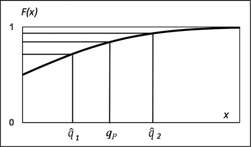
Consider the fundamental characteristic of a quantile. illustrates the standardized normal distribution and two estimates1 and
2 for quantile qP. When measured horizontally,
1 is closer to qP than
2, but F(
2) is closer to F(qP) than F(
1). The essential role of a quantile qP is to answer the question: “What is the probability for a random x not to exceed qP?” In this respect,
2 performs much better than
1 because |F(
2)-F(qP)|< |F(
1)-F(qP)|. The fact that |
1 - qP |< |
2 - qP| is irrelevant when the probability is concerned. In other words, the goodness of estimate
i is defined by |F(
i)-F(qP)|, not by |
i - qP |. This simple consideration implies that all goodness criteria for quantile estimators, based on the distance measured along X-axis, are dubious. When concepts such as mean, bias, mean squared error etc. are used in X-direction for comparison of quantiles, the concept of probability is lost. The criterion for “close to”, based on the distance measured along P-axis, is preferable because that distance is proportional to the number of hits in a MC simulation, i.e., proportional to the probability. In “Criteria for quantile estimators” section, this aspect is considered in more detail.
Figure 1. Two estimates 1 and
2 for qP.
1 is closer to qP than
2 but F(
2) is closer to F(qP) than F(
1).
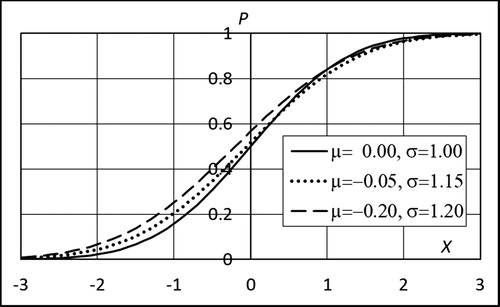
Using the same arguments, any other criterion based on the deviation of a quantile estimate from the correct value is dubious. As an example, consider a normal distribution N(μ,σ) = N(0,1) illustrated in . Over the most part of the range, the estimated dotted curve is closer to the exact curve than the estimated dashed curve. This seems natural because the parameters of the dotted curve are closer to the exact ones than those of the dashed curve.
Figure 2. Curves for normal distributions with mean μ and standard deviation σ.
However, if we look at the upper tail illustrated in , the dashed curve is better than the dotted curve both in vertical and horizontal directions. Even more striking is the fact that “improving” the dotted curve by setting μ = 0.0 enlarges the range where the dashed curve is better than the dotted one, as seen in . Particularly in extreme value analysis, the upper tail of the distribution is crucial. Nevertheless, it is not uncommon to base the conclusions concerning the quantile estimators on minimization of the bias of the distribution parameters.
Figure 3. Upper tail of the curves in .
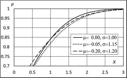
Figure 4. Same as , but the dotted curve is an “improvement” of the dotted curve in the previous figure.

Let us consider one more example which deals with the bias of the parameter estimators. It is well-known that when the MLE is applied to a sample from exponential distribution
(1)
(1)
MLE yields a biased estimate
for λ . If, for example,
= 2, we may conclude that
should be abandoned. On the other hand, applying MLE to the same sample, but writing
(2)
(2)
we get
= ½. Again,
but this time
may be regarded excellent because
is unbiased. This “paradox” can be explained in a simple way. Even though quantiles can be estimated by estimating the distribution parameters, the quantile estimators cannot be assessed based on the bias of the parameter estimators.
3. Criteria for quantile estimators
3.1. Classical approaches
Given a continuous random variable X with probability distribution F, an arbitrary value q0 of X and probability p0, the validity of hypothesis q0 = F−1(p0) can be tested by generating K random numbers y1,…,yK from X and observing, what happens to the ratio rK = (number of yi not exceeding q0)/K when K increases without limit. When E(rK), the expected value of rK, equals p0, we say that F(q0) = p0 by definition of the classical probability.
Logics require that a criterion for the goodness of a quantile estimator must be based on the definition of a quantile. Since the quantiles define the distribution function, the same requirement applies to the goodness of the estimator of the distribution function.
In practical situations, we are not interested in testing whether an arbitrary value of x equals F−1(p0), and we do not know F. Instead, we have a sample S = {x1,…,xN}, i.e., a set of observations from X. To determine quantiles, we need an estimator T that is a rule associating, to any S and probability p, a quantile estimate P. We may formally write T(S,p) =
P. The performance or goodness of an estimator may depend on F and p, but not on the set of observations we happen to have. The performance of T for a certain distribution F is assessed by generating a great number of sets Si = {xi,1,…,xi,N} (samples of size N) and using a criterion which tells how well T performs on average. In the same way as “close to” has several interpretations, “on average” have been understood in many ways. Some examples of this are given below.
Cunnane (Citation1978) postulated that the order statistics xi from a known distribution type F with unknown parameters shall be associated to the plotting positions (probabilities) pi = F(E(Xi)). He also preferred the MLS in X-direction because in this way the mean squared error (MSE) of the quantiles is minimized. The values of pi can numerically be evaluated when N and the form of F are known. They depend on the size of the sample and on the form of F. It follows that T defined by T(S,pi) = Pi = xi is an unbiased estimator of pi-quantile because F−1(pi) = E(Xi) = qPi. However, as pointed out in Chapter 2 above, such an unbiased estimator is not in line with the definition of a quantile.
Minimizing the MSE of the distribution parameters is the goodness criterion favored e.g., by Chernoff and Lieberman (Citation1954), and minimizing the bias of the distribution parameters was preferred e.g., by Fuglem, Parr, and Jordaan (Citation2013). Fuglem, Parr, and Jordaan (Citation2013) carried out MC simulations with the linear MLS for several distribution types and plotting positions. They concluded that the Weibull plotting with pi = i/(N + 1) should not be used because it results in more biased estimators for distribution parameters, as well as for 0.9- and 0.99-quantiles, than the other plotting positions. However, as pointed out above and discussed further below, an estimator that aims at unbiased distribution parameters may be a poor estimator of the quantiles.
Maximum likelihood (MLE) and the moment methods (MM) perform well in minimizing the bias or MSE of quantiles, and they have been widely recommended in the literature and used in practice, see e.g., Castillo (Citation1988) and Millar (Citation2011). We stress again that such criteria are not probabilistically sound goodness criteria for quantile estimators.
3.2. Measure of the goodness of an estimator based on the definition of a quantile
To illustrate the difference in performance of two goodness criteria, three examples are given in the following. From order statistics we know that if S = {x1,…,xN} is an order- ranked sample from random variable X and y is an arbitrary value of X, the probability of event A = {y ≤ xi} is equal to i/(N + 1), see e.g., Madsen, Krenk, and Lind (Citation1986), Makkonen, Pajari, and Tikanmäki (Citation2012) and Makkonen and Pajari (Citation2014). Obviously, xi is an ideal estimator for i/(N + 1)-quantile. For example, choosing N = 99 implies that x50, x98 and x99 are ideal estimators for 0.50, 0.98- and 0.99-quantiles, respectively. To compare the criteria in which either the bias of the cumulative probability of the quantile or that of the quantile itself is minimized, 10 000 samples from Gumbel, and log-normal distributions are taken and the expected value evaluated using data given in . To give an impression of the effect of the sample size, one case with N = 29 is also considered. The results are shown in .
Figure 5. Simulated expectation for the 0.5-quantile (median) and for the cumulative probability of the median. Gumbel distribution, sample sizes 29 and 99.
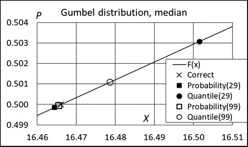
Figure 6. Simulated expectation for the 0.98-quantile and cumulative probability of the quantile. Gumbel distribution, sample size 99.
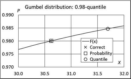
Figure 7. Simulated expectation for the 0.99-quantile and cumulative probability of the quantile. Lognormal distribution, sample size 99.
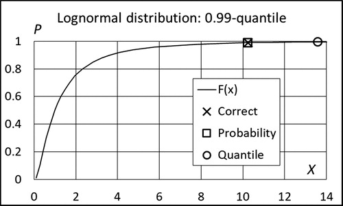
Table 1. Quantile simulations.
As expected, in all of the examples in the cumulative probability of any considered quantile is unbiased, but the quantile itself is biased. This demonstrates that a goodness criterion aiming at minimum bias of the quantile estimator results in an estimate of the quantile, which contradicts the definition of the quantile. For example, in the case illustrated in , the 0.9900-quantile is x = 10.2. The expectation of the quantile estimate x99 is then x = 13.6 which, in fact, is the 0.9955-quantile. It also follows that (10.2/13.6) x99 = 0.75x99 should be an unbiased estimator for the 0.99-quantile, which underlines the absurdity of the unbiased quantile estimators.
The examples above represent discrete quantiles, which depend on the size of the sample. In practice, quantiles are often searched for p-values which do not equal i/(N + 1). For these cases, let F be the CDF of a random variable X. Define experiment as generating a random number y from X. According to the classical frequency interpretation, the probability of event A = {y ≤ qp} is
(3)
(3)
where p is a given probability, qp = F−1(p) and #K(Z) is the number of events Z in K subsequent experiments. qp is called the p-quantile of X.
Let T be a quantile estimator which transforms a given probability p and sample S = (x1,…,xN) from X into a CDF in such a way that
(4)
(4)
where the quantile estimate of p is
Define experiment now as: given F and p, generate N random numbers x1,…,xN from X, use the given estimator T to find
and
and generate one more random number y from X. In one experiment, the probability of an event
= {y ≤
} is
(5)
(5)
In subsequent K experiments, K different values of
are obtained. An ideal estimator would yield
(6)
(6)
where #K(Z) is the number of events Z in K experiments. Hence, when K is high, the difference
(7)
(7)
is a natural measure of the goodness of the quantile estimator T for F and p. This is the case in MC simulations in which the number of cycles (experiments) can be made large enough to achieve convergence. Furthermore, if dK does not converge to zero with increasing K, the estimator is erroneous. In this sense, dK presents a unique measure for the goodness of quantile estimators.
The goodness of an estimator may depend on the probability distribution F, probability p and the size of the sample, but the same measure of the goodness can be used to compare the different quantile estimators.
Consider next the estimation of the quantile difference qp2 - qp1 where p1 < p2 and F(qp1) = p1, F(qp2) = p2. Let be the estimated CDF and
(8)
(8)
EquationEquation (6)
(6)
(6) means that the probability of event
=
is
(9)
(9)
The difference
(10)
(10)
is a good measure for the goodness of the estimator for the probability of event
when K is large. In other words, when the number of simulations in a MC simulation is large, the number of hits between
and
divided by the number of simulations is the appropriate estimate for the probability of event B =
3.3. Fundamental property of probability distribution function applied to quantile estimation
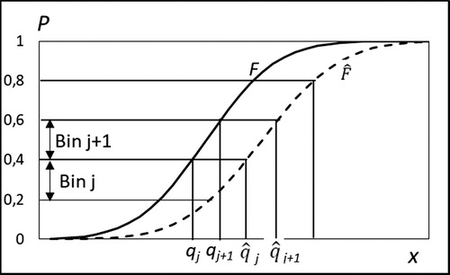
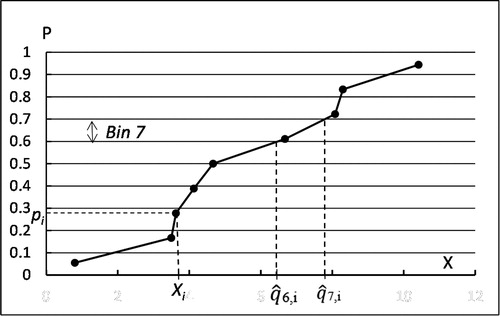
illustrates a fundamental property of a continuous distribution function F: Let us cut the probability axis with J + 2 equally spaced horizontal lines at Pj = j/(J + 1), j = 0(1)(J + 1), and call the interval (Pj-1, Pj] bin j or Bj when j = 1(1)(J + 1). Now, when taking randomly K values y1,…,yK from X, then rj, the share of hits of yk values in interval (qj-1,qj] =(F−1(Pj-1), F−1(Pj)] approaches stochastically 1/(J + 1) with increasing K. This property provides the means for comparison of an estimated distribution with the exact distribution. Such a comparison is based on the same idea as Pearson’s well-known χ2-statistic.
Figure 8. Five bins. Bin limits on X- and P-axis for exact (F) and estimated distribution ().
To evaluate the accuracy of an estimated distribution we take K random numbers y1,…,yK from X and calculate rj, the share of hits in bin Bj using bin limits
=
−1(pj) instead of qj = F−1(pj). A nearly uniform distribution of rj in the bins with increasing K tells that the pj-quantiles of
are nearly exact, i.e.,
−1(pj) ≈ F−1(pj). The deviation
(11)
(11)
is a robust measure of the accuracy of the estimated pj-quantile
because it tells us how much the cumulative probability of the estimated quantile
=
−1(pj) deviates from the correct value pj. Note that the number and size of the bins, with obvious modifications in EquationEquation (11)
(11)
(11) may be chosen arbitrarily.
3.4. Bin criterion for goodness of quantile estimators
A criterion, based on the fundamental property of quantiles, and aimed for comparison of different quantile estimators, is introduced in the following. We call it the bin criterion. This criterion is applied to estimators of the whole distribution function but can also be used for single quantiles. There are similarities between the bin criterion and the discrete die-rolling process for checking the fairness of a die and in the MC simulation for assessing a quantile estimator of a continuous random variable X with distribution F. compares these two processes and their goodness criteria.
Table 2. Comparison of rolling a die and bin simulation for a distribution estimator.
An overall criterion for an estimator is the mean squared error of relative bin frequencies
(12)
(12)
It is obvious that a quantile estimator T that meets this bin criterion is unbiased in regard to the probability of pj-quantile estimates
K may be = 1, but a higher value of K speeds up the convergence of rj, particularly for estimators which need much computer time per cycle.
The bin criterion, with obvious modifications, works with non-equal bin sizes as well. For example, to compare the goodness of two estimators T1 and T2 for a given p-quantile, we set J = 1, and B1 = [0,p], B2 = (p,1], and let K be a large number in a MC simulation. Then dmse,i = [(ri,1 – p)2 + (ri,2 – 1+p)2]/2 and the smaller of values dmse,1, dmse,2 indicates the better estimator.
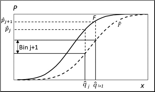
As shown in , instead of generating y1,i,…,yK,i from X as in , the probability of a random number from X to fall in bin Bj can directly be calculated from (see )
(13)
(13)
Figure 9. The probability of a random y from F(x) to fall in bin j + 1 is j+1 -
j.
The share of hits in Bj then becomes
(14)
(14)
This method is recommended to speed up the convergence. The generation of random numbers y1,i,…,yK,i was introduced first above, because it is similar to the die-rolling process and illustrates the close relation of the bin criterion to Pearson’s χ2-statistic which, when applied to a case with sample size K and J + 1 equal bins, gives
(15)
(15)
Both dmse and χ2 represent the same idea. Given the number (J + 1) of equal bins and the size of the sample (K), only the difference in the number of observed and theoretical hits in the bins matters. However, there are some differences regarding the use of these two statistics. When applying χ2, a probability distribution is assumed correct in the 0-hypothesis, and the statistic is typically used to check whether one sample of size K is taken from that distribution, whether two samples are taken from the same distribution etc. However, dmse is used for comparison of estimators. For such a comparison, a great number of samples is taken from X with a known distribution, and there is no need to check where the samples come from. The goodness of the estimators can then be evaluated based on dmse. This can be done even when no critical values of the statistic dmse are specified.
4. Applying the bin criterion to broken line estimators
Associating “probabilities” p’1,…,p’N (plotting positions) to order-ranked observations x1,…,xN, respectively, and plotting the corresponding points (xi,p’i) on a probability paper has been considered briefly above. Traditionally, this has been a visual method for checking whether the observations are in accordance with the distribution specific to the probability paper used. If the points seem to be on a straight line, the distribution assumption is regarded as correct and the parameter estimates are solved from the slope and intersection of the line.
The Weibull positions p’i = i/(N + 1) are a natural choice because the probability of a random x not to exceed xi equals i/(N + 1), see e.g., Madsen, Krenk, and Lind (Citation1986), Makkonen, Pajari, and Tikanmäki (Citation2012), and Makkonen and Pajari (Citation2014). In other words, i/(N + 1) is in full agreement with the definition of the cumulative distribution function. This result is independent of the underlying distribution F. Nevertheless, many other plotting positions depending on F and N have been proposed, recommended and used, because the bias of some Weibull-based estimators concerning both the quantiles and distribution parameters can be reduced in this way. However, as shown in Chapter 2, abandoning the Weibull plotting positions due to such a bias is unfounded.
illustrates the principle of MC simulations with N = 9 order statistics x1,…,x9. Points (xi,p’i) where p’i is the plotting position chosen for comparison, are connected to their neighbors with straight lines. A broken line estimate is obtained. The broken line is cut by horizontal lines at p = pj = j/(J + 1). Choosing J = N simplifies the MC simulation. (J < N is also possible. J > N would not be useful because the broken line might not intersect the highest and lowest horizontal lines.) The cutting points determine the estimated quantiles
j,i or bin limits. K new random numbers yk are taken from X. The share of the number of hits of yk in each bin Bj is recorded. Repeating the cycle described above and summing up the number of hits in each bin, a reliable comparison between the estimators with different plotting positions can be made.
Figure 10. Determining bin limits for cumulative probability distribution.
The principles presented above were followed in a number of simulations with J = N = 30, K = 1 and M = 106. The probability distributions in were used. The results of these simulations are shown in and illustrated in for the normal distribution. As expected, the Weibull plotting works well, the other alternatives are poor. The measure dmse gets bigger the further the plotting positions are from the Weibull positions. This shows that the criteria for the goodness of broken line estimators proposed by Hyndman and Fan (Citation1996) are not in accordance with the bin criterion. In contrast to the conclusions by Hyndman and Fan (Citation1996), plotting positions other than those of Weibull clearly give an erroneous picture of the CDF.
Figure 11. MC simulation for normal distribution N(0,1). Number of hits in bins 1,…, 31.
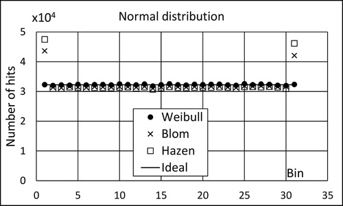
Table 3. Cumulative distribution functions (CDF) used in the numerical simulations.
Table 4. Results of MC simulations for normal, log-normal, exponential and Gumbel distribution.
These MC simulations support the conclusion made above that the Weibull plotting positions are the only ones that are based on the concept of probability. Abandoning the other historically used plotting positions greatly simplifies the estimation based on plotting. When applying the Weibull plotting, the goodness of the estimators depends only on the goodness of the curve fitting.
In the early days of order statistics, when applying the MLS on probability paper with Weibull plotting, it was observed that the bias in distribution parameters or quantiles was high, or some other desirable property was not achieved. The natural step, modifying the curve-fitting method alone, was not taken. Instead, the plotting positions were varied to meet the preferred statistical requirements. Since then, the distortion due to the curve fitting and nonlinear scaling of the probability axis have been compensated by opposite errors in the plotted points to which the curve has been fitted (Makkonen Citation2008).
The broken line estimator connects pi = i/(N + 1) with the order statistic xi. It is well-known that E(F(Xi)) = i/(N + 1) is true for all F (Gumbel Citation1958). This means that, when using the Weibull plotting, the broken line estimator is unbiased when interpreted as an estimator of random variables F(Xi). The resulting quantile estimators are biased, but in probabilistic sense this is irrelevant.
5. Applying bin criterion to probability distributions fitted to a sample
5.1. The simulation tools
A free mathematical program (Sage, version 4.3), was used for generation of random numbers and solving the distribution parameters when using the method of least squares (scipy.optimize, least squares, trf) or maximum likelihood estimator (scipy.optimize, minimize, BFGS). When the MLE is applied to normal and exponential distribution, or when the linear MLS regression is applied to find the parameters of a distribution, an explicit solution is obtained. When this is not possible, a solution may be found using a suitable iterative algorithm, but the convergence is not guaranteed. In the following analysis, a sample resulting in divergent iteration has been replaced by a new sample until the target number of solutions (=105) has been achieved.
5.2. Probability distribution estimated by method of least squares in the P-direction
We carried out a MC simulation based comparison similar to that in the previous section but, instead of a broken line through the plotted points, the distribution was estimated by a curve fitted using the MLS in the P-direction without scaling of the probability axis. This results in nonlinear regression in P-direction.
The results of the MC simulations with 105 samples of size 15 and 30 for the 4 distributions are given in . EquationEquation (15)(15)
(15) was applied to find the share of hits in each bin. As expected, the Weibull plotting positions perform best except for Weibull distribution with sample size of 15. For the other plottings, dmse increases with increasing distance from the Weibull’s plotting positions. Additional simulations on the Weibull distribution showed that for sample sizes greater than 27 the Weibull plotting results in a lower value of dmse than the other plotting positions.
Table 5. Results of MC simulations for some distributions.
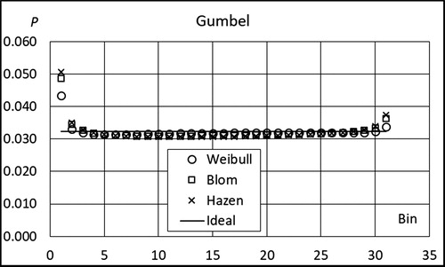
and show the probability of a random x to fall in bins 1,…,31 when the sample size is 30. The points for Cunnane and Gringorten plotting are not shown but they lie between those of Blom and Hazen. The first and last bins have a pronounced role. For Weibull plotting, this is different from the broken line estimators, see , and reflects the incomplete behavior of the MLS. With increasing sample size this effect becomes weaker.
Figure 12. Probability of a random x from Normal distribution to fall in bins 1,…, 31.
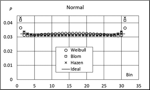
Figure 13. Probability of a random x from Gumbel distribution to fall in bins 1,…, 31.
5.3. Probability distribution estimated by method of least squares in X-direction
For some probability distributions, a technical advantage of the MLS in X-direction is the possibility to use linear regression without nonlinear scaling of the P- or X-axis or both. As shown in , this may be an appropriate choice even when the probability and the random variable are not linearly related. The results show that, for the normal, Gumbel and Weibull distributions, the Weibull plotting is a good choice, but not for the exponential distribution.
Table 6. Results of MC simulations for some distributions.
5.4. Comparison of maximum likelihood method and method of least squares
In we compare, using the bin criterion, the maximum likelihood estimator (MLE) and the method of least squares (MLS) with Weibull plotting. The least squares are calculated in the P-direction using scaled P-axis (“probability paper approach”) and without scaling, as well as in the X-direction without scaling.
Table 7. Simulations with 105 samples of size 15.
Table 8. Same as , but with samples size of 30.
Table 9. Same as , but with sample size of 100 and without the last column.
The results in and show that the classic probability paper approach, where the P-axis is scaled, is not competitive at all. Interestingly, the accuracy of the MLS with Weibull plotting, both in X-direction and in P-direction without scaling of P-axis, is competitive with the accuracy of the MLE, and in most cases considerably better. This property remains the same for sample size 100 as shown in . Thus, for small sample sizes, i.e., when the errors are significant, MLS outperforms MLE.
5.5. Bias of distribution parameter estimates
During the MC simulations described in “Comparison of maximum likelihood method and method of least squares” section, the mean of the parameter values obtained in subsequent simulations was also recorded. The simulated means are shown in , where each of the values is the mean of 105 parameter values obtained using MLE and MLS with Weibull plotting in the P-direction without scaling. Since the MLE is inaccurate for sample sizes of the order of 15, the corresponding values were not calculated.
Table 10. Mean of distribution parameters in simulations. N is the sample size.
shows that when increasing the sample size, the mean of the estimated parameters seems to approach the corresponding value of the parent distribution given in . However, this does not happen with a constant sample size and with increasing number of samples. This means that the parameter values obtained using the MLE or MLS are slightly biased, as one would expect based on the discussions in “Performance of quantile estimators” section.
5.6. Cumulative bin distribution function as a goodness measure for a single quantile
Statistic dmse reflects the overall performance of a quantile estimator. For a given quantile, comparison of the discrete “cumulative bin distribution function” ϕ
(16)
(16)
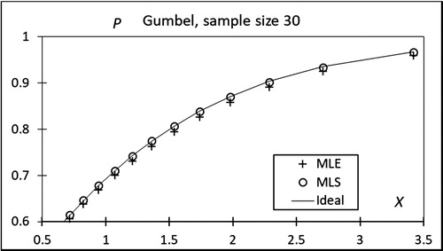
with the parent distribution F gives a better illustration of the goodness of the considered estimator for that specific quantile. This is illustrated in and for the Gumbel distribution. For small values of the observed variable X, MLE and MLS in the P-direction with Weibull plotting appear almost equally good, but the MLS is clearly better for high values of X, which is the important range in which Gumbel distribution is applied to the extreme value analysis.
Figure 14. Cumulative bin distribution function compared with CDF of the parent Gumbel distribution.
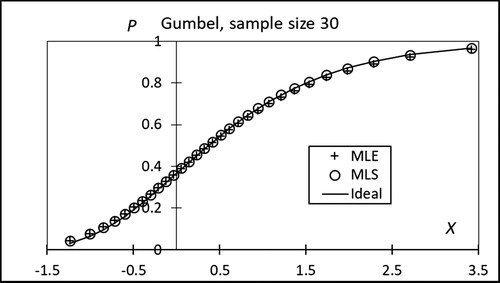
Figure 15. Upper right corner of .
6. Conclusions
The background of the Makkonen-Pajari-Tikanmäki bin statistic dmse for assessing quantile estimators was clarified in this paper. The proposed bin statistic dmse is based on the definition of probability in the same sense as Pearson’s χ2 statistic. It provides a measure for assessing the goodness of quantile estimators, which is in accordance with the definition of the cumulative distribution function. The bin statistic can be used both for a single quantile and for the distribution function, i.e., for the whole range of quantiles of a continuous random variable.
We showed that the criteria traditionally used to assess the quantile estimators, such as minimization of the bias or mean squared error of the quantiles themselves or those of the distribution parameters, should be abandoned. They violate the probability theory, because they are determined by the distance between the estimate and the correct value measured by a concept other than probability. Such a distance is a concept alien to the definition of a quantile, and should not be used when evaluating the performance of quantile estimators.
The focus of the present paper was to introduce and justify the bin criterion for assessing the goodness of fit and demonstrate how it is used. In this connection, the weaknesses of the classical estimation methods became evident. As an interesting byproduct, our Monte-Carlo simulations by applying the bin criterion showed that, when the P-axis is not scaled, the Method of Least Squares with Weibull plotting is a better estimator than the Maximum Likelihood Method.
Additional information
Funding
References
- Castillo, E. 1988. Extreme value theory in engineering. San Diego: Academic Press.
- Chernoff, H., and G. J. Lieberman. 1954. Use of normal probability paper. Journal of the American Statistical Association 49 (268):778–85. doi:10.2307/2281539.
- Cunnane, C. 1978. Unbiased plotting positions - a review. Journal of Hydrology 37 (3-4):205–22. doi:10.1016/0022-1694(78)90017-3.
- Fuglem, M., G. Parr, and I. J. Jordaan. 2013. Plotting positions for fitting distributions and extreme value analysis. Canadian Journal of Civil Engineering 40:1–3. doi:10.1139/cjce-2012-0427.
- Gringorten, I. I. 1963. A plotting rule for extreme probability paper. Journal of Geophysical Research 68 (3):813–14. doi:10.1029/JZ068i003p00813.
- Gumbel, E. J. 1958. Statistics of extremes. New York: Columbia University Press.
- Hyndman, R. J., and Y. Fan. 1996. Sample quantiles in statistical packages. The American Statistician 50:361–65. doi:10.2307/2684934.
- Madsen, H. O., S. Krenk, and N. C. Lind. 1986. Methods of structural safety. Englewood Cliffs, New Jersey: Prentice-Hall. doi:10.1016/0167-4730(86)90028-7.
- Makkonen, L. 2008. Bringing closure to the plotting position controversy. Communications in Statistics - Theory and Methods 37 (3):460–67. doi:10.1080/03610920701653094.
- Makkonen, L., M. Pajari, and M. Tikanmäki. 2012. Closure to “Problems in the extreme value analysis.” Structural Safety 40:65–67. doi:10.1016/j.strusafe.2012.09.007.
- Makkonen, L., and M. Pajari. 2014. Defining sample quantiles by the true rank probability. Journal of Probability and Statistics 326579. doi:10.1155/2014/326579.
- Makkonen, L., and M. Tikanmäki. 2019. An improved method of extreme value analysis. Journal of Hydrology X 2:100012. doi:10.1016/j.hydroa.2018.100012.
- Millar, R. B. 2011. Maximum likelihood estimation and inference. Hoboken, New Jersey: Wiley.