Detecting long-range dependence with truncated ratios of periodogram ordinates

Abstract

We propose new tests for testing hypotheses about the memory parameter that are based on ratios of periodogram ordinates. They are highly robust against conditional heteroskedasticity and outliers and are therefore of great value for the detection of long-range dependence in financial data. The robustness is obtained by truncation of a distribution with nonexistent moments. Tables of critical values are provided. The performance of the new tests is assessed by extensive simulations. Applying the tests to daily series of gold price returns and stock index returns, we find no evidence of long-range dependence characterized by a non-vanishing memory parameter. In the case of spread series (differences between interest rates at different maturities, gold prices and silver prices, related stock market indices), we find no evidence of a memory parameter well below 0.5.

Keywords:

• Memory parameter
• Periodogram
• Robust tests
• Truncated F distribution

MATHEMATICS SUBJECT CLASSIFICATION:

• 62M10
• 62M15
• 62P20
• 62Q05

1. Introduction

Let ${(y_t)}_{t\in \mathbb{Z}}$ be a fractionally integrated ARMA (ARFIMA) process satisfying (1) $${(1-L)}^d\mathrm{\Phi }\left(L\right)y_t=\mathrm{\Theta }\left(L\right)u_t$$(1)

(Granger and Joyeux 1980; Hosking 1981), where $d<0.5$ (stationarity condition), $d>-0.5$ (invertibility condition), $L$ is the lag operator, all roots of the polynomials $\mathrm{\Phi }\left(L\right)=1-{\varphi }_{1}L-\dots -{\varphi }_p{L}^p$ and $\mathrm{\Theta }\left(L\right)=1-{\theta }_{1}L-\dots -{\theta }_q{L}^q$ lie outside the unit circle (causality condition and invertibility condition, respectively), the fractional difference operator ${(1-L)}^d$ is defined by the expansion (2) $${(1-L)}^d=1-dL+d\left(d-1\right)L^2/2-d(d.1)(d-2)L^3/3!+\dots$$(2) and ${(u_t)}_{t\in \mathbb{Z}}$ is a white noise process with mean 0 and variance ${\sigma }^2.$ The negative signs in $\mathrm{\Theta }\left(L\right)$ are due to the unusual parametrization for the MA part in the R package ‘fracdiff’, which will be employed in our simulation study to generate realizations of ARFIMA processes. Since the autocorrelation function $\rho \left(h\right)=\mathit{Cor}(y_{t+h},y_t)$ of an ARFIMA process with $0<\left|d\right|<0.5$ decays more slowly as $h\to \infty$ than that of an ARMA process ($d=0$), the former process is said to exhibit long-range dependence (or long memory) and the latter is said to exhibit short-range dependence (or short memory). In order to distinguish between ARFIMA processes with positive and negative values of the memory parameter (or fractional differencing parameter) $d,$ the latter are sometimes said to exhibit antipersistence (or intermediate memory or negative memory). For a review of several formal definitions of long memory see Palma (2007).

The spectral density of the stationary ARFIMA process (1)(1) $${(1-L)}^d\mathrm{\Phi }\left(L\right)y_t=\mathrm{\Theta }\left(L\right)u_t$$(1) is given by (3) $$f\left(\omega \right)=\frac{{\sigma }^2}{2\pi }{\left|1-e^{-i\omega }\right|}^{-2d}{\left|1-\sum _{j=1}^q{\theta }_j{e}^{-i\omega j}\right|}^2{\left|1-\sum _{j=1}^p{\varphi }_j{e}^{-i\omega j}\right|}^{-2}, \omega \in \left(-\pi ,\pi \right]$$(3) which reduces to the familiar ARMA spectral density (4) $$f_0\left(\omega \right)=\frac{{\sigma }^2}{2\pi }{\left|1-\sum _{j=1}^q{\theta }_j{e}^{-i\omega j}\right|}^2{\left|1-\sum _{j=1}^p{\varphi }_j{e}^{-i\omega j}\right|}^{-2}, \omega \in \left(-\pi ,\pi \right]$$(4) if $d=0.$

When an ARFIMA process is used as a model for a time series $y_1{,\dots ,y}_n,$ the model dimension ($p,1,q)$ must be specified and the model parameters ${d,\varphi }_1,\dots ,{\varphi }_p,$${\theta }_1,\dots ,{\theta }_q,{\sigma }^2$ must be estimated. If the model is correctly specified, maximum likelihood (ML) estimation of the model parameters is the method of choice (see Dahlhaus 1989; Sowell 1992; for an estimation procedure that is based on the approximate maximum likelihood see Fox and Taqqu 1986). However, the model dimension is unknown in practice. If a misspecified model is chosen, the ML estimator will be inconsistent. Robinson (1995) and Reschenhofer (2013) therefore argued that it is safer to take a nonparametric approach (e.g., rescaled range analysis; see Hurst 1951; Mandelbrot 1971; Hauser and Reschenhofer 1995) or a semiparametric approach (e.g., the log periodogram regression of Geweke and Porter-Hudak 1983, the local Whittle likelihood of Künsch 1987, the averaged periodogram of Robinson 1994a, the smoothed periodogram of Reisen 1994 the wavelet analysis of Abry and Veitch 1998 and Moulines, Roueff, and Taqqu 2007).

Hurvich, Deo, and Brodsky (1998) established the asymptotic normality (5) $$\sqrt{K}\left(\widehat{d}-d\right)\stackrel{d}{\to }N\left(0,\frac{{\pi }^2}{24}\right)$$(5) of the log periodogram estimator (6) $$\widehat{d}={\sum }_{j=1}^K{(x}_j-\overline{x})\log I\left({\omega }_j\right)/S_{xx}$$(6) where (7) $${\mathrm{ }x}_j=-2\mathrm{ }\log \left|1-e^{-i\omega }\right|=-\mathrm{ }2\mathrm{ log}\left(\text{sin}({\omega }_j/2)\right)$$(7) and ${\omega }_j=2\pi j/n$ is the j’th Fourier frequency, for the case where $K=o(n^{4/5})$ and ${\log }^2\left(n\right)=o(K).$ When K is small, approximate normality may not hold because the central limit theorem has not kicked in yet. Conducting a Monte Carlo power study with small and medium values of K, Mangat and Reschenhofer (2019) found that conventional tests that are based on the asymptotic normality of the log periodogram estimator either have extremely low power (when the standard variance formula ${(\pi }^2/6)/S_{xx}$ of the least squares estimator of the slope in a simple linear regression is used instead of the asymptotic variance) or do not attain the advertised levels of significance (when the asymptotic variance ${\pi }^2/24$ is used). They therefore further developed Bartlett’s (1954, 1955) frequency-domain test for white noise, which is based on the application of the Kolmogrov-Smirnov test (for a standard uniform distribution) to the cumulative sum (8) $$\sum _{j=1}^{r}I\left({\omega }_j\right)/\sum _{j=1}^{m}I\left({\omega }_j\right), r=1,\dots ,m-1,\mathrm{ }m=\left[\right(n-1)/2]$$(8) by using only Fourier frequencies ${\omega }_j$ in the neighborhood of frequency zero and dividing each periodogram ordinate $I({\omega }_j)$ by ${\omega }_j^{-2d_0}$ in order to allow the testing of hypotheses such as $H_0:d=d_0,$ $H_0:d\ge d_0,$ and $H_0:d\le d_0.$ The Kolmogrov-Smirnov test is particularly suitable for the testing of these hypotheses because the cumulative sum (8)(8) $$\sum _{j=1}^{r}I\left({\omega }_j\right)/\sum _{j=1}^{m}I\left({\omega }_j\right), r=1,\dots ,m-1,\mathrm{ }m=\left[\right(n-1)/2]$$(8) is approximately linear under the null hypothesis and is either concave or convex under the alternative hypothesis, which is exactly that framework in which the Kolmogrov-Smirnov test is most powerful (whereas it may have extremely low power against more complex alternatives; see Reschenhofer and Bomze 1991; Reschenhofer 1997). While the test proposed by Mangat and Reschenhofer (2019) performs well in the case of small samples (and has the further advantage that no new tables of critical values have to be provided), its applicability to financial time series is impacted negatively by its sensitivity to non-normality and conditional heteroskedasticity (see Section 3). The goal of this paper is therefore to develop tests that do not only function properly in the case of small samples but are also robust against conditional heteroskedasticity and heavy tails. Tests with these properties are introduced in Sec. 2 before their performance is examined with the help of a Monte Carlo power study in Sec. 3. Section 4 applies the robust tests to financial time series. Section 5 concludes.

2. Robust tests and estimators

2.1. Simple expressions for the moments of a truncated F distribution

In the following, we obtain simple expressions for the mean and the variance of a truncated $F(2$)-distribution, which will be then used in Subsection 2.2 to construct robust tests of hypotheses about the memory parameter d.

After restricting the support of an ${F(\nu }_1,{\nu }_2$)-distribution with density $g\left(x\right)$ and distribution function $G\left(x\right)$ to the interval $\left(C,D\right),$ the density of the truncated distribution ${F_{[C,D]}(\nu }_1,{\nu }_2$) becomes (9) $$\begin{array}{c}f\left(x\right)=\frac{1}{G\left(D\right)-G\left(C\right)}\mathrm{ }g\left(x\right)\\ =\frac{1}{G\left(D\right)-G\left(C\right)}\mathrm{ }{\frac{1}{B\left(\frac{{\nu }_1}{2},\frac{{\nu }_2}{2}\right)}\mathrm{ }\left(\frac{{\nu }_1}{{\nu }_2}\right)}^{\frac{{\nu }_1}{2}}\frac{x^{\frac{{\nu }_1}{2}-1}\mathrm{ }}{{\left(1+\frac{{\nu }_{1}x}{{\nu }_2}\right)}^{\frac{{\nu }_1+{\nu }_2}{2}}},\end{array}\mathrm{ }$$(9) where ${\nu }_1>0,$ ${\nu }_2>0,$ $-\infty \le C<x<D\le \infty ,$ and B is the beta function defined by (10) $$B\left(u,v\right)=\frac{\mathrm{\Gamma }\left(u\right)\mathrm{\Gamma }\left(v\right)}{\mathrm{\Gamma }\left(u+v\right)}, u,\mathrm{ }v\in \mathbb{C}, Re\left(u\right)>0, Re\left(v\right)>0$$(10)

Nadarajah and Kotz (2008) derived explicit expressions for the moments of this truncated distribution in terms of the ordinary hypergeometric function represented by the Gauss hypergeometric series (11) $${\mathrm{ }}_2{F}_1\left(a,b;c;z\right)=\sum _{j=0}^{\mathrm{\infty }}\frac{{\left(a\right)}_j{\left(b\right)}_j}{{\left(c\right)}_j}\frac{z^j}{j!}=1+\frac{ab}{c·1}z+\frac{a(a+1)b(b+1)}{c(c+1)·1·2}{z}^2+\dots$$(11) where $\left|z\right|<1$ and ${(a)}_j=a\left(a+1\right)\dots (a+j-1)$ denotes the ascending factorial. This series is not defined if $c$ is a nonpositive integer and neither $a$ nor $b$ is a nonpositive integer that is greater than $c$ (see Gradshteyn and Ryzhik 2007, 1005). If X has a truncated ${F(\nu }_1,{\nu }_2$)-distribution, then (12) $$\begin{array}{c}E{X}^n=\frac{1}{G\left(D\right)-G\left(C\right)}\mathrm{ }\frac{1}{B\left(\frac{{\nu }_1}{2},\frac{{\nu }_2}{2}\right)}\mathrm{ }\frac{2{\nu }_1^n}{{\nu }_2^n(2n+{\nu }_1)}\\ \begin{array}{c}\times \left[\mathrm{ }\frac{{\left({\nu }_{1}D\right)}^{n+\frac{{\nu }_1}{2}}}{{{(\nu }_2+{\nu }_{1}D)}^{n+\frac{{\nu }_1}{2}}}\right.{\mathrm{ }}_2{F}_1\left(n+\frac{{\nu }_1}{2},1+n-\frac{{\nu }_2}{2};1+n+\frac{{\nu }_1}{2};\frac{{\nu }_{1}D}{{(\nu }_2+{\nu }_{1}D}\right)\\ \left.-\frac{{\left({\nu }_{1}C\right)}^{n+\frac{{\nu }_1}{2}}}{{{(\nu }_2+{\nu }_{1}C)}^{n+\frac{{\nu }_1}{2}}}{\mathrm{ }}_2{F}_1\left(n+\frac{{\nu }_1}{2},1+n-\frac{{\nu }_2}{2};1+n+\frac{{\nu }_1}{2};\frac{{\nu }_{1}C}{{(\nu }_2+{\nu }_{1}C}\right)\right]\end{array}\end{array}$$(12) where (13) $$\begin{array}{c}G\left(D\right)-G\left(C\right)=\frac{{2\left({\nu }_{1}D\right)}^{\frac{{\nu }_1}{2}}}{{{{\nu }_1(\nu }_2+{\nu }_{1}D)}^{\frac{{\nu }_1}{2}}}{\mathrm{ }}_2{F}_1\left(\frac{{\nu }_1}{2},1-\frac{{\nu }_2}{2};1+\frac{{\nu }_1}{2};\frac{{\nu }_{1}D}{{\nu }_2+{\nu }_{1}D}\right)\\ -\frac{{2\left({\nu }_{1}C\right)}^{\frac{{\nu }_1}{2}}}{{{{\nu }_1(\nu }_2+{\nu }_{1}C)}^{\frac{{\nu }_1}{2}}}{\mathrm{ }}_2{F}_1\left(\frac{{\nu }_1}{2},1-\frac{{\nu }_2}{2};1+\frac{{\nu }_1}{2};\frac{{\nu }_{1}C}{{\nu }_2+{\nu }_{1}C}\right)\end{array}$$(13)

For $C=0$ and $D=1$ and ${\nu }_1={\nu }_2=2,$ we obtain (14) $$G\left(D\right)-G\left(C\right)=G\left(1\right)=\mathrm{ }\frac{1}{2}{\mathrm{ }}_2{F}_1\left(1,\mathrm{ }0;2;\mathrm{ }\frac{1}{2}\right)=\frac{1}{2}$$(14) (15) $${\mu }_{tF}=EX=\frac{1}{4}{\mathrm{ }}_2{F}_1\left(2,\mathrm{ }1;3;\mathrm{ }\frac{1}{2}\right)=2\log \left(2\right)-1\mathrm{ }\sim \mathrm{ }0.3862944$$(15) (16) $$E{X}^2=\frac{1}{12}{\mathrm{ }}_2{F}_1\left(3,\mathrm{ }2;4;\mathrm{ }\frac{1}{2}\right)=\frac{1}{6}{\mathrm{ }}_2{F}_1\left(1,\mathrm{ }2;4;\mathrm{ }\frac{1}{2}\right)=3-4\log \left(2\right)\sim \mathrm{ }0.2274113$$(16) and (17) $${\sigma }_{tF}^2=\mathit{Var}\left(X\right)=E{X}^2-{\left(EX\right)}^2=2-4{\log }^2\left(2\right)\sim \mathrm{ }0.07818794$$(17) because (18) $$\begin{array}{c}\frac{1}{4}{\mathrm{ }}_2{F}_1\left(2,\mathrm{ }1;3;z\right)=\frac{1}{4}\left(1+\frac{2}{3}z+\frac{2}{4}{z}^2+\frac{2}{5}{z}^3+\dots \right)\\ =\frac{1}{2z^2}\left(z+\frac{z^2}{2}+\frac{z^3}{3}+\frac{z^4}{4}+\frac{z^5}{5}+\dots \right)-\frac{1}{2z}\\ =-\frac{\log (1-z)}{2z^2}-\frac{1}{2z}\end{array}$$(18) (19) $${\mathrm{ }}_2{F}_1\left(a,b;c;z\right)={(1-z)}^{c-a-b}{\mathrm{ }}_2{F}_1\left(c-a,c-b;c;z\right)$$(19)

(see Gradshteyn and Ryzhik 2007, 1008), and (20) $$\begin{array}{c}{\mathrm{ }}_2{F}_1\left(1,\mathrm{ }2;4;z\right)=1+\frac{2}{4}z+\frac{2·3}{4·5}{z}^2+\frac{2·3}{5·6}{z}^3+\dots \\ =1+\frac{2}{4}z+\frac{2·3}{z^2}\left(\frac{z}{1·2}+\frac{z^2}{2·3}+\frac{z^3}{3·4}+\frac{z^4}{4·5}+\frac{z^5}{5·6}+\dots \right)-\frac{2·3}{z^2}\left(\frac{z}{1·2}+\frac{z^2}{2·3}+\frac{z^3}{3·4}\right)\\ =1+\frac{2}{4}z+\frac{2·3}{z^2}\left(1-\frac{1-z}{z}\mathrm{ }\log \left(\frac{1}{1-z}\right)\right)-\mathrm{ }\frac{2·3}{z^2}\left(\frac{z}{1·2}+\frac{z^2}{2·3}+\frac{z^3}{3·4}\right)\mathrm{ }\end{array}$$(20)

2.2. Test statistics, critical values and asymptotic distributions

Under the simple (but in many applications implausible) assumption that the observations $y_1{,\dots ,y}_n$ are i.i.d. normal with mean 0 and variance ${\sigma }^2,$ the normalized periodogram ordinates $J\left({\omega }_j\right)=2\pi {\sigma }^{2}I\left({\omega }_j\right),$ $1\le j\le m=[(n-1)/2],$ are i.i.d. standard exponential and the ratios $R_{j,k}=J\left({\omega }_j\right)/J\left({\omega }_k\right)=I\left({\omega }_j\right)/I\left({\omega }_k\right),$ $j\ne k,$ have an $F(2\mathrm{,}2$)-distribution. Since the moments of this distribution do not exist (not even the first one), we truncate the ratios $R_{j,k}$ to the interval (0,1). The mean ${\mu }_{tF}$ and the variance ${\sigma }_{tF}^2$ of the truncated ratios are then given by (15)(15) $${\mu }_{tF}=EX=\frac{1}{4}{\mathrm{ }}_2{F}_1\left(2,\mathrm{ }1;3;\mathrm{ }\frac{1}{2}\right)=2\log \left(2\right)-1\mathrm{ }\sim \mathrm{ }0.3862944$$(15) and (17)(17) $${\sigma }_{tF}^2=\mathit{Var}\left(X\right)=E{X}^2-{\left(EX\right)}^2=2-4{\log }^2\left(2\right)\sim \mathrm{ }0.07818794$$(17) , respectively.

If the spectral density of the data generating process is not constant but strictly increasing on the interval $(0,\pi ),$ e.g., in the case of an AR(1) process with ${\varphi }_1<0,$ then each ratio $R_{j,k}$ with $j<k$ will asymptotically be distributed as a constant ${\lambda }_{j,k}<1$ times an $F(2\mathrm{,}2$)-distribution, which implies that (21) $$P\left(R_{j,k}<1\right)>0.5$$(21)

because the median of an $F(2$)-distribution is 1, and (22) $$E\left(\left.R_{j,k}\right|R_{j,k}<1\right)<{\mu }_{tF}$$(22) because the probability density function of an $F(2$)-distribution is a convex function and the truncated density of $R_{j,k}$ is therefore steeper than that of the truncated $F(2$)-distribution. Given a subset S of the set (23) $$S_K^{-}=\left\{R_{j,k}:1\le j<k\le K\le m\right\}$$(23) we could use both the proportion of ratios that fall into the interval [0,1] - because of (21)(21) $$P\left(R_{j,k}<1\right)>0.5$$(21) - and the sample mean of those ratios - because of (22)(22) $$E\left(\left.R_{j,k}\right|R_{j,k}<1\right)<{\mu }_{tF}$$(22) - to test the null hypothesis of white noise against the alternative hypothesis of a strictly increasing spectral density. Choosing a subset such as $\left\{R_{1,2},R_{3,4},R_{5,6},\dots \right\}\subseteq S_K^{-}$ or $\left\{R_{1,2},R_{3,6},R_{4,8},R_{5,10},R_{7,14},\dots \right\}\subseteq S_K^{-}$ has the advantage that its elements are independent and the central limit theorem can be applied to the sample mean $\overline{R}$(S) of those $n_{[0,1]}$ elements of S that fall into the interval [0,1], which entails that the test statistic (24) $$T_S^{-}=\sqrt{n_{[0,1]}\mathrm{ }}\frac{\overline{R}-{\mu }_{tF}}{{\sigma }_{tF}}$$(24) will approximately have a standard normal distribution under the null hypothesis if $n_{[0,1]}$ is large. The null hypothesis will be rejected by this one-sided test if the test statistic $T_S^{-}$ takes a too large negative value. Indeed, in case of a strictly increasing spectral density, the term $n_{[0,1]}$ in will be larger than under the null hypothesis because of (21)(21) $$P\left(R_{j,k}<1\right)>0.5$$(21) and the term $\overline{R}-{\mu }_{tF}$ will be a large negative number because of (22)(22) $$E\left(\left.R_{j,k}\right|R_{j,k}<1\right)<{\mu }_{tF}$$(22) .

Analogously, when we suspect that the spectral density of the data generating process is strictly decreasing on the interval $(0,\pi ),$ e.g., in the case of an AR(1) process with ${\varphi }_1>0,$ then each ratio $R_{j,k}$ with $j<k$ will asymptotically be distributed as a constant ${\lambda }_{j,k}>1$ times an $F(2\mathrm{,}2$)-distribution, which implies that $P\left(R_{j,k}<1\right)<0.5$ and $E\left(\left.R_{j,k}\right|R_{j,k}<1\right)>{\mu }_{tF}.$ In this case, we could replace $n_{[0,1]}$ in (24)(24) $$T_S^{-}=\sqrt{n_{[0,1]}\mathrm{ }}\frac{\overline{R}-{\mu }_{tF}}{{\sigma }_{tF}}$$(24) by $\left|S\right|-n_{[0,1]}$ and reject the null hypothesis if the resulting test statistic takes a too large positive value. Note that under the null hypothesis $n_{[0,1]}/(\left|S\right|-n_{[0,1]})$ will converge in probability to 1 because the $F\left(2,2\right)$-distribution has a median of 1. However, since the test statistic will generally be more informative when the sample mean is based on a larger sample, we prefer to stick to (24)(24) $$T_S^{-}=\sqrt{n_{[0,1]}\mathrm{ }}\frac{\overline{R}-{\mu }_{tF}}{{\sigma }_{tF}}$$(24) and only replace all ratios $R_{j,k}$ with $j<k$ by $R_{k,j}.$ The set $\left\{R_{k,j}:1\le j<k\le K\le m\right\}$ will be denoted by $S_K^{+}$ and the associated test statistic based on a subset S of $S_K^{+}$ by $T_S^{+}.$

When our focus is on small samples, tables of critical values are more important than the asymptotic distribution, hence there is no need to keep the dependence structure simple. In the following, we will therefore, in order to increase the power of our tests, use the whole sets $S_K^{-}$ and $S_K^{+},$ respectively, instead of just simple subsets. Obviously, for the two tests $T_K^{-}$ and $T_K^{+}$ that are based on the sets $S_K^{-}$ and $S_K^{+},$ respectively, we need only one set of critical values. Table 1 gives the 0.05%, 1%, 2.5%, 5%, 95%, 97.5%, 99%, and 99.5% quantiles for $m=5, 6, 7, 8, 9, 10, 15, 20, 24, 25, 50, 100, 150.$ The quantiles in each column of this table were obtained by generating 10,000,000 random samples of size $m$ from the standard exponential distribution, evaluating the test statistic $T^{-}$ for each random sample, and finally computing the order statistics of the sample of 10.000.000 values of $T^{-}.$

Table 1. Critical values for the tests based on the test statistics $T^{-}$ and $T^{+}.$

	K = 5	6	7	8	9	10	15	20	24	25	50	100	150
0.05%	−2.702	−2.881	−3.139	−3.358	−3.499	−3.712	−4.406	−5.174	−5.503	−5.802	−8.340	−11.500	−13.932
1%	−2.479	−2.697	−2.934	−3.057	−3.257	−3.402	−4.084	−4.657	−5.026	−5.344	−7.488	−10.279	−12.733
2.50%	−2.205	−2.371	−2.534	−2.661	−2.805	−2.929	−3.524	−4.041	−4.275	−4.454	−6.260	−8.748	−10.828
5%	−1.907	−2.039	−2.159	−2.273	−2.396	−2.475	−2.992	−3.438	−3.669	−3.739	−5.346	−7.425	−9.056
95%	2.159	2.342	2.450	2.590	2.789	2.854	3.240	3.815	4.095	4.050	5.503	7.673	9.507
97.50%	2.551	2.758	2.890	3.083	3.277	3.415	3.954	4.499	5.021	4.872	6.630	9.336	11.377
99%	2.957	3.225	3.429	3.719	3.860	4.035	4.654	5.322	5.904	5.740	7.827	11.250	13.925
99.50%	3.205	3.657	3.832	4.087	4.304	4.401	5.137	5.862	6.507	6.382	8.728	12.466	15.258

The critical values from Table 1 can also be used to test hypotheses about the memory parameter d of an ARFIMA(0,d,0) process (fractionally integrated white noise). In this framework, the normalized periodogram ordinates $J\left({\omega }_j\right)=I\left({\omega }_j\right)/f\left({\omega }_j\right),$ $H\le j\le K,$ are asymptotically i.i.d. standard exponential provided that $H$ is not too small (recall the discussion in Sec. 1) and the ratios (25) $$R_{j,k}\left(d\right)=\frac{I\left({\omega }_j\right)/{\left|1-e^{-i\omega }\right|}^{-2d}}{I\left({\omega }_k\right)/{\left|1-e^{-i\omega }\right|}^{-2d}}=\frac{I\left({\omega }_j\right)}{I\left({\omega }_k\right)}·{\left(\frac{\text{sin}({\omega }_j/2)}{\text{sin}({\omega }_k/2)}\right)}^{2d}\sim \mathrm{ }\frac{I\left({\omega }_j\right)}{I\left({\omega }_k\right)}·{\left(\frac{{\omega }_j/2}{{\omega }_k/2}\right)}^{2d}=\frac{I\left({\omega }_j\right)}{I\left({\omega }_k\right)}·{\left(\frac{j}{k}\right)}^{2d}$$(25) depend only on the unknown parameter $d,$ hence the null hypothesis $d\ge d_0$ can be rejected if the test statistic (26) $$T_K^{-}\left(d\right)=\sqrt{n_{[0,1]}\mathrm{ }}\frac{\overline{R}\left(d\right)-{\mu }_{tF}}{{\sigma }_{tF}}$$(26)

takes a too large negative value, where $n_{[0,1]}$ is the number of elements of (27) $$S_K^{-}\left(d\right)=\left\{R_{j,k}\left(d\right):1\le j<k\le K\le m\right\}$$(27) that fall into the interval [0,1] and $\overline{R}(d)$ is the sample mean of these elements. Analogously, the test statistic $T_K^{+}(d)$ can be defined when we want to test the null hypothesis that $d\le d_0.$

When we use the first $K$ Fourier frequencies, they become smaller and smaller as the sample size $n$ increases. Clearly, the very lowest frequencies, which are the most informative with regard to long-range dependence, are the ones which are closest to frequency zero. Unfortunately, the distribution of the periodogram at these very frequencies is out of line (Künsch 1986; Hurvich and Beltrao 1993; Robinson 1995). Omitting the first $H$ Fourier frequencies, where H grows with n, is an obvious option. Indeed, if $(H+1)/\sqrt{n}\to \infty$ and $(H+K)/n\to 0,$ the normalized periodogram ordinates $J\left({\omega }_{H+1}\right),\dots , J\left({\omega }_{H+K}\right)$ will still be asymptotically i.i.d. standard exponential (Künsch 1986). Clearly, the choice of H is critical. For example, ${H=[n}^{0.6}/50]$ satisfies Künsch’s condition but equals zero for n = 100. In their simulation studies, Reisen, Abraham, and Lopes (2001) and Mangat and Reschenhofer (2019) found that even for much larger values of n, keeping the lowest Fourier frequencies is harmless, which is in line with the results of our own simulation study presented in Sec. 3. We conclude that for sample sizes typically occurring in practice, it is safe to set $H=0.$

The condition $(H+K)/n\to 0$ (or $K/n\to 0$ if $H=0$) is crucial when the observations come from a general ARFIMA process rather than from fractionally integrated white noise. K must not be too large to ensure that we are not misled by the behavior of the spectral density outside a neighborhood of frequency zero (short-range dependence), which is described by the AR parameters ${\varphi }_1,\dots ,{\varphi }_p$ and the MA parameters ${\theta }_1,\dots ,{\theta }_q$ (whereas the memory parameter d describes the behavior close to frequency zero and therefore takes care of any long-range dependence).

Although frequency-domain methods are in general more robust than time-domain methods (because periodogram ordinates are squares of sums whereas sample autocovariances are sums of squares or products), their performance may deteriorate in the presence of volatility clusters and extreme observations, which are typical for financial time series. We may expect that our frequency-domain tests, which are based on the truncated ratios of normalized periodogram ordinates, are more robust. Our simulation study, which will be presented in the next section, shows that this is indeed the case.

3. Simulations

In order to examine the robustness of our tests, we allow for deviations from normality, homoscedasticity, and uncorrelatedness. For this purpose, we use submodels of the ARFIMA(p,d,q)-GARCH(1,1) model (28) $${{(1-L)}^d\left(1-{\varphi }_{1}L\right)y}_t=\left(1-{\theta }_{1}L\right)u_t$$(28) where $$p+q\le 1$$ $$u_t={\sigma }_t{z}_t$$ $$z_t\sqrt{\nu /(\nu -2)}\mathrm{ }\text{i.i.d.}\mathrm{ }t\left(\nu \right) \text{with} \nu =5$$ $${\sigma }_t^2={\alpha }_0+{\alpha }_1{u}_{t-1}^2+{\beta }_1{\sigma }_{t-1}^2$$

α₀=1, α₁=0.1, β₁=0.8999

Short-range dependence is controlled by the parameters ${\varphi }_1$ and ${\theta }_1.$ Nonnormality is accomplished by using a distribution with heavier tails, namely the t-distribution, rather than by introducing additive outliers. Conditional heteroscedasticity is modeled by a simple GARCH(1,1) model because the focus of this simulation study is on robustness only and not on the modeling of real financial data. For the latter purpose, more sophisticated models that are able to capture asymmetry in the returns as well as long memory and periodicities in the volatility would be more appropriate than simple GARCH models (see Nelson 1991; Baillie, Bollerslev, and Mikkelsen 1996; Lopes and Prass 2013, 2014). The model (28)(28) $${{(1-L)}^d\left(1-{\varphi }_{1}L\right)y}_t=\left(1-{\theta }_{1}L\right)u_t$$(28) becomes increasingly ill-behaved (heavier tails, fewer existing moments, more distinct volatility patterns) as the number $\nu$ of degrees of freedom decreases and the sum α₁+β₁ approaches 1. The fourth moment of a $t(\nu )$-distribution exists if $\nu >4.$ However, for the existence of the fourth unconditional moment of the GARCH(1,1) process $u_t$ it is required that (29) $$E{\left({\beta }_1+{\alpha }_1{z}_{t-1}^2\right)}^2<1$$(29) (see Nelson 1990; He and Teräsvirta 1999). If $z_{t-1}\sqrt{\nu /(\nu -2)} \sim t\left(\nu \right)$ and $\nu =5,$ we have (30) $$E{\left({\beta }_1+{\alpha }_1{z}_{t-1}^2\right)}^2={\beta }_1^2+2{\beta }_1{\alpha }_1+9{\alpha }_1^2$$(30) which is already greater than one for α₁=0.1 and β₁=0.86. Vošvrda and Žikeš (2004) fitted an GARCH(1,1) model to the returns of the Warsaw Stock Exchange Index (which will also be analyzed in the next section) and obtained the estimates 0.082, 0.854, 6.521 for the parameters α₁, β₁, and $\nu .$ By choosing a small value of $\nu$ and α₁+β₁ very close to 1, we ensured the occurrence of both extreme values and large volatility fluctuations. The results of our simulation study therefore allow to draw conclusions about the robustness of our tests, which use critical values that have been obtained under the idealized assumption that the normalized periodogram ordinates are indeed independent and standard exponentially distributed.

For the generation of a large number of pseudorandom samples of size $n=250$ from the model (28)(28) $${{(1-L)}^d\left(1-{\varphi }_{1}L\right)y}_t=\left(1-{\theta }_{1}L\right)u_t$$(28) , we used the function ‘fracdiff.sim’ from the R package ‘fracdiff’ with a burn in period of length 5,000. For each of 5,000 samples generated with $d_A=-0.4, -0.3, \dots , 0.3,$ the null hypotheses $H_0:d\ge d_0$ with $d_0=d_A+0.1, d_A+0.2,\dots ,0.4$ were tested using the test statistic $T_a^{-}$ with $K=\left[\sqrt{n}\right]=15.$ Analogously, for each of 5,000 samples generated with $d_A=-0.4, -0.3, \dots , 0.4,$ the null hypotheses $H_0:d\le d_0$ with $d_0=-0.4,-0.3, \dots ,d_A$ were tested using the test statistic $T_a^{+}$ with $K=15.$ Table 2 shows the rejection rates at the (one-sided) 5% level of significance for $p=q=0.$ Results obtained for alternatives with non-zero values of ${\varphi }_1$ and ${\theta }_1$ are shown in Table 3. In general, the power is relatively low if $d_0$ is close to $d_A$ but increases quickly as the distance between $d_0$ and $d_A$ increases. The values in the main diagonal are reasonably close to 5%, which suggests that our tests roughly attain the advertised levels of significance even in case of serious deviations from normality and homoscedasticity. The only exceptions occur in the case of large values of ${\varphi }_1,$ where we would need larger sample sizes (e.g., $n=1000$) to distinguish between short-range autocorrelation and long-range autocorrelation.

Table 2. Rejection rates (at the 5% level of significance) obtained by applying the tests (with $K=15$) based on the test statistics $T_a^{-}$ (if $d_A<d_0)$ and $T_a^{+}$ (if $d_A\ge d_0),$ respectively, to samples of size $n=250$ from an ARFIMA(0,d,0)-GARCH(1,1) model with $t(5)$ distributed innovations and GARCH parameters α₀ = 1, α₁ = 0.1, β₁ = 0.8999.

d0\dA	−0.4	−0.3	−0.2	−0.1	0.0	0.1	0.2	0.3	0.4
−0.4	0.054	0.093	0.142	0.238	0.355	0.480	0.626	0.753	0.842
−0.3	0.076	0.056	0.080	0.144	0.230	0.343	0.489	0.633	0.747
−0.2	0.121	0.081	0.047	0.088	0.144	0.226	0.345	0.492	0.623
−0.1	0.197	0.131	0.071	0.056	0.083	0.141	0.224	0.349	0.487
0.0	0.302	0.216	0.121	0.082	0.050	0.087	0.133	0.235	0.357
0.1	0.441	0.328	0.206	0.142	0.077	0.052	0.075	0.137	0.223
0.2	0.587	0.468	0.317	0.219	0.133	0.080	0.045	0.082	0.134
0.3	0.728	0.615	0.459	0.331	0.221	0.132	0.077	0.046	0.072
0.4	0.842	0.754	0.617	0.487	0.330	0.218	0.133	0.076	0.045

Table 3. Rejection rates (at the 5% level of significance) obtained by applying the tests (with $K=15$) based on the test statistics $T_a^{-}$ (if $d_A<d_0)$ and $T_a^{+}$ (if $d_A\ge d_0),$ respectively, to samples of size $n=250$ from an ARFIMA(p,d,q)-GARCH(1,1) model with $t(5)$ distributed innovations, GARCH parameters α₀ = 1, α₁ = 0.1, β₁ = 0.8999, and different values of (a) the AR parameter ${\varphi }_1$ and (b) the MA parameter ${\theta }_1,$ respectively.

(a) p = 1, q = 0
d0\dA		−0.4			−0.2			0			0.2			0.4
ϕ1	0.25	0.50	0.75	0.25	0.50	0.75	0.25	0.50	0.75	0.25	0.50	0.75	0.25	0.50	0.75
−0.4	0.06	0.07	0.15	0.15	0.17	0.35	0.35	0.42	0.65	0.65	0.69	0.86	0.87	0.9	0.97
−0.2	0.12	0.09	0.05	0.05	0.06	0.14	0.15	0.17	0.36	0.36	0.4	0.64	0.67	0.71	0.88
0	0.3	0.26	0.13	0.12	0.1	0.05	0.05	0.06	0.15	0.14	0.17	0.35	0.39	0.42	0.66
0.2	0.58	0.54	0.32	0.31	0.27	0.13	0.13	0.11	0.05	0.05	0.06	0.15	0.17	0.18	0.38
0.4	0.84	0.81	0.61	0.61	0.55	0.32	0.31	0.27	0.14	0.13	0.1	0.05	0.07	0.06	0.15
(b) p = 0, q = 1
d0\dA		−0.4			−0.2			0			0.2			0.4
θ1	0.25	0.50	0.75	0.25	0.50	0.75	0.25	0.50	0.75	0.25	0.50	0.75	0.25	0.50	0.75
−0.4	0.06	0.05	0.03	0.13	0.11	0.06	0.33	0.28	0.14	0.63	0.56	0.35	0.85	0.81	0.63
−0.2	0.12	0.14	0.18	0.05	0.04	0.02	0.13	0.1	0.05	0.33	0.28	0.14	0.63	0.57	0.35
0	0.31	0.33	0.39	0.13	0.17	0.3	0.04	0.04	0.02	0.13	0.1	0.05	0.34	0.29	0.15
0.2	0.59	0.61	0.66	0.34	0.4	0.57	0.14	0.17	0.34	0.05	0.04	0.02	0.14	0.11	0.05
0.4	0.85	0.85	0.87	0.64	0.69	0.83	0.35	0.4	0.63	0.14	0.18	0.34	0.05	0.04	0.02

The values corresponding to those shown in Table 2 are less favorable for the non-robust test employed by Mangat and Reschenhofer (2019) for the detection of long-range dependence in series of gold price returns and stock index returns. E.g., for $d_0=-0.4$ and $d_A=-0.4,$ 0.1, 0.2, 0.3, 0.4, the probability to reject the true null hypothesis is 0.069 and the probabilities to reject the false null hypotheses are 0.374, 0.480, 0.587, and 0.671, respectively (compared to the values 0.054 and 0.480, 0.626, 0.753, 0.842 from Table 2). The non-robust test may therefore be of limited usefulness in financial applications. In the next section, we will reanalyze the gold and stock index data sets with our robust tests. In addition, we will have a look at several spread series.

4. Empirical results

Recent studies found indications of time-varying long memory in financial time series (Cajueiro and Tabak 2004; Carbone, Castelli, and Stanley 2004; Hull and McGroarty 2014; Auer 2016b). Batten et al. (2013) and Auer (2016a) explored possible applications for the development of profitable trading strategies. They used estimates of the Hurst coefficient $H,$ which is related to the memory parameter $d$ via $H=d+0.5,$ for the generation of buy and sell signals. Batten et al. (2013) used the values –0.1 and 0.1 as thresholds (for estimates of $d,$ i.e., 0.4 and 0.6 for estimates of $H$) and a rolling window of 22 trading days. In an effort to reduce transactions costs by reducing the trading frequency, Auer (2016a) increased the threshold values to –0.2 and 0.2 and the window size to 240 trading days. However, in the light of the results of our simulation study (see Section 3), it seems virtually impossible to distinguish between close neighboring values such as –0.1, 0, and 0.1 and still extremely difficult to distinguish between –0.2, 0, and 0.2. The worst case for any trading strategy based on fractal dynamics is when there is no long-range dependence at all, i.e., $d=0$ throughout the whole observation period. Mangat and Reschenhofer (2019) applied their non-robust tests to series of gold price returns and stock index returns in a rolling analysis and found that the overall pattern of rejections could best be explained by the absence (or virtual absence) of long-range dependence. In the following, we will apply our new robust tests to the same datasets and check whether we arrive at the same conclusion.

Daily gold prices from 1979-01-01 to 2017-11-10 were downloaded from the website www.gold.org of the World Gold Council. Daily quotes of the Dow Jones Industrial Average (DJIA) from 1928-10-02 to 2018-02-07 were obtained from Yahoo!Finance. Using the test statistics $T_a^{-}$ and $T_a^{+}$ to test the hypotheses $H_0:d\ge 0.2$ and $H_0:d\le -0.2$ at the 5% level of significance in a rolling analysis with a window size of 250 trading days and $K=15,$ we obtained the rejection rates 0.124 and 0.062, respectively, for the gold price returns and 0.126 and 0.128, respectively, for the stock index returns. Apart from the second one, these rates agree well with the results obtained in our simulation study for $d_A=0$ (see Table 2). The agreement is even better, when a higher value of $K$ is used. In Figure 1, the rejection rates obtained for $K=24$ are plotted cumulatively. 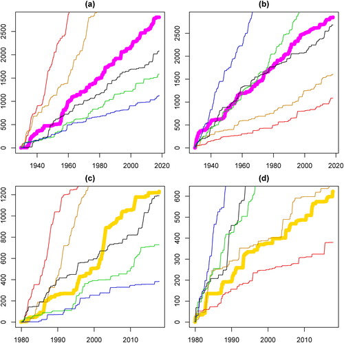Clearly, similar rejection rates would also be obtained if there was a balanced ratio between values of $d$ greater than 0.2 on the one hand and less than –0.2 on the other hand. However, given competing explanations for a particular outcome, the simplest explanation is often the correct one (Occam's razor). Moreover, Figure 1 shows no indications of structural breaks in the memory parameter.

Figure 1. Cumulative number of rejections with $n=250,$ $K=24,$ α = 0.05 by tests based on $T_a^{-}$ with $d_0=0.2$(a,c) and $T_a^{+}$ with $d_0=-0.2$(b,d): gold returns (bold in gold), DJIA returns (bold in magenta), synthetic ARFIMA(0,d,0)-series with $d=-0.2$ (red), $d=-0.1$ (orange), $d=0$ (darkgray), $d=0.1$ (green), $d=0.2$ (blue).

While using only a small set of Fourier frequencies in a rolling analysis to distinguish between different values of $d$ that lie close to each other may not promise success, there are other interesting problems which are easier to solve. In the absence of any evidence of fractal dynamics, we can use the whole sample and in further consequence include more Fourier frequencies in order to increase the power of our tests and narrow down the range of possible values of $d.$ In the following, we consider four financial time series consisting of thousands of observations (as opposed to the sample size of 250 in our rolling analysis). However, we increase the number of included Fourier frequencies only moderately in order to safeguard against possibly more complex short-range dependence. In accordance with reports in the literature (see the discussion above) about possible long-range dependence in returns series of emerging markets and in spread series, the first of our four time series contains the log returns of the Warsaw Stock Exchange Index (WIG) from 2011-03-11 to 2019-04-12 (downloaded from Investing.com) and the other three time series are potentially (trend) stationary differences of two nonstationary time series, i.e., the difference of the log Amsterdam Exchange Index ($̂$ AEX) and the log BEL 20 Index ($̂$ BFX) from 1991-04-09 to 2017-12-12, the trend residuals obtained from the difference of the CBOE 10 Year Treasury Yield Index ($̂$ TNX) and the CBOE 5 Year Treasury Yield Index ($̂$ 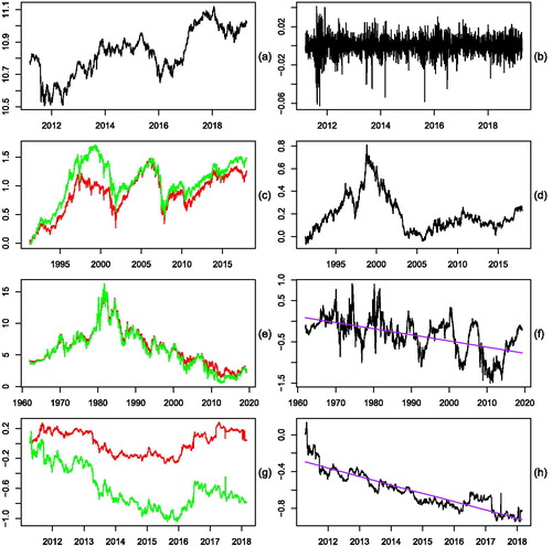FVX) from 1962-01-02 to 2019-04-12 (see Figure 2f), and, finally, the trend residuals obtained from the difference of the log iShares Physical Gold ETC (SGLN.L) and the log iShares Silver ETC (SSLN.L) from 2011-04-14 to 2018-02-27 (all downloaded from Yahoo! Finance). The last time series was truncated at 2018-02-27 because of too many missing values in the last part. Figure 2a, c, e, and g show the original time series and Figure 2b, d, f, and h show the return series and spread series, respectively.

Figure 2. (a) Log Warsaw Stock Exchange Index, (b) Log returns, (c) Log Amsterdam Exchange Index (green) & log BEL 20 Index (red), (d) Difference, (e) 5 Year Treasury Yield Index (green) & 10 Year Treasury Yield Index (red), (f) Difference, (g) Log iShares Physical Gold ETC (green) & log iShares Silver ETC (red), (h) Difference.

Ideally, the parameter d in the true data generating model should not be too close to 0 in the case of the returns series and not too close to 0.5 in the case of the spread series in order to keep a good chance of obtaining significant and interpretable results. However, testing the null hypothesis that $d\le 0.4$ for the difference of the stock market indices, the test statistic $T_a^{+}$ with $K=25,$ 50, 100, 150 took the values −7,206 (**), −14.272 (**), −25,883 (**), −42,947 (**), where (*) indicates significance at the 5% level and (**) significance at the 1% level. The corresponding values for the term spread and the gold-silver spread were −3,681, −6,943 (*), −11,792 (**), −20,198 (**) and −4,0318 (*), −8,302 (**), −13,191 (**), −32,4636 (**), respectively. Accordingly, it was never possible to reject the converse hypothesis that $d\ge 0.4,$ which would have implied that the two original series were fractionally cointegrated (see Robinson 1994b; Caporale and Gil-Alana 2004). Finally, assuming that $d=0$ in the case of the returns series, the best we could hope for was to rule out values of d that are too far from 0. Indeed, using the test statistic $T_a^{+}$ ($T_a^{-}$), the null hypothesis that $d\le -0.3$ ($d\ge 0.3)$ could be rejected at the 1%-level with $K=150.$

5. Discussion

Being interested primarily in financial applications, our focus is on simple ARFIMA models with small p and $q=0$ or small q and $p=0,$ which helps us to avoid the problem that reliable inference on the memory parameter is not possible if the unrestricted class of all ARFIMA models is used. Indeed, Pötscher (2002) has shown that the maximum risk of any estimator ${\widehat{d}}_n$ for the memory parameter d, which is based on a sample of size n, is bounded from below by a positive constant independent of n, i.e., (31) $$\sup E{\left|{\widehat{d}}_n-d\right|}^r\ge \frac{1}{2^r}>0$$(31) where $1\le r<\infty$ and the supremum is taken over all Gaussian ARFIMA processes.

Another critical issue is the choice of the number of Fourier frequencies used for testing. Since conventional frequency-domain tests for log-range dependence assume that the number of used Fourier frequencies grows with the sample size, which is not reasonable in case of a rolling analyses of a long time series, and the test proposed by Mangat and Reschenhofer (2019) which is based on a fixed number of Fourier frequencies, does not attain the advertised levels of significance in case of deviations from normality and homoscedasticity, we have developed robust tests that are based on truncated ratios of periodogram ordinates at a fixed set of Fourier frequencies. The truncation is crucial for the robustness of the tests and the existence of moments. Overall, there are four robust tests. The first two are less powerful but have simple asymptotic distributions. The other two tests are more sophisticated. Because they are closely related, we provide only one set of critical values which can be used for both tests. The choice between the two tests depends on the alternative hypothesis we have in mind, i.e., it depends whether we think that the memory parameter of the data generating model is greater or less than the values specified under the null hypothesis.

We conducted a simulation study to investigate the power of our tests and, in particular, to check whether they attain the advertised levels of significance in the presence of outliers and conditional heteroskedasticity. The results suggest that the answer to the latter question is affirmative, which indicates that the tests are indeed highly robust. Regarding the power, the findings are less favorable. With the specifications likely to be used in a rolling analysis, e.g., $n=250$ and $K=15,$ it may be difficult to distinguish between values of $d$ that are too close to each other, e.g., –0.2, 0, and 0.2. However, if we use the whole time series and values of K such as 50, 100, or 150, we may be able to narrow down the range of possible values of d. In our empirical investigation of various financial time series, we could reject the hypotheses $d\le -0.3$ and $d\ge 0.3$ for return series and the hypothesis $d\le 0.4$ for spread series.

Acknowledgments

The authors thank two anonymous reviewers for helpful suggestions and comments.

References

- Abry, P., and D. Veitch. 1998. Wavelet analysis of long-range-dependent traffic. IEEE Transactions on Information Theory 44 (1):2–15. doi:10.1109/18.650984.
- Auer, B. R. 2016a. On the performance of simple trading rules derived from the fractal dynamics of gold and silver price fluctuations. Finance Research Letters 16:255–67. doi:10.1016/j.frl.2015.12.009.
- Auer, B. R. 2016b. On time-varying predictability of emerging stock market returns. Emerging Markets Review 27:1–13. doi:10.1016/j.ememar.2016.02.005.
- Baillie, R., T. Bollerslev, and H. Mikkelsen. 1996. Fractionally integrated generalized autoregressive conditional heteroskedasticity. Journal of Econometrics 74 (1):3–30. doi:10.1016/S0304-4076(95)01749-6.
- Bartlett, M. 1954. Problèmes de l'analyse spectrale des séries temporelles stationnaires. Publications de l'Institut de statistique de l'Université de Paris 3:119–34.
- Bartlett, M. 1955. An introduction to stochastic processes with special reference to methods and applications. Cambridge: Cambridge University Press.
- Batten, J., C. Ciner, B. Lucey, and P. Szilagyi. 2013. The structure of gold and silver spread returns. Quantitative Finance 13 (4):561–70. doi:10.1080/14697688.2012.708777.
- Cajueiro, D., and B. Tabak. 2004. The Hurst exponent over time: Testing the assertion that emerging markets are becoming more efficient. Physica A: Statistical Mechanics and Its Applications 336 (3–4):521–37. doi:10.1016/j.physa.2003.12.031.
- Caporale, G. M., and L. A. Gil-Alana. 2004. Fractional cointegration and tests of present value models. Review of Financial Economics 13 (3):245–58. doi:10.1016/j.rfe.2003.09.009.
- Carbone, A., G. Castelli, and H. E. Stanley. 2004. Time-dependent Hurst exponent in financial time series. Physica A: Statistical Mechanics and Its Applications 344 (1–2):267–71. doi:10.1016/j.physa.2004.06.130.
- Dahlhaus, R. 1989. Efficient parameter estimation for self-similar processes. The Annals of Statistics 17 (4):1749–66. doi:10.1214/aos/1176347393.
- Fox, R., and M. S. Taqqu. 1986. Large-sample properties of parameter estimates for strongly dependent stationary Gaussian time series. The Annals of Statistics 14 (2):517–32. doi:10.1214/aos/1176349936.
- Geweke, J., and S. Porter-Hudak. 1983. The estimation and application of long memory time series models. Journal of Time Series Analysis 4 (4):221–38. doi:10.1111/j.1467-9892.1983.tb00371.x.
- Gradshteyn, I. S., and I. M. Ryzhik. 2007. Table of integrals, series, and products (7th edition, ed. A. Jeffrey and D. Zwillinger). Amsterdam: Elsevier/Academic Press.
- Granger, C. W. J., and R. Joyeux. 1980. An introduction to long-memory time series models and fractional differencing. Journal of Time Series Analysis 1 (1):15–29. doi:10.1111/j.1467-9892.1980.tb00297.x.
- Hauser, M. A., and E. Reschenhofer. 1995. Estimation of the fractionally differencing parameter with the R/S method. Computational Statistics & Data Analysis 20:569–79. doi:10.1016/0167-9473(94)00062-N.
- He, C., and T. Teräsvirta. 1999. Properties of moments of a family of GARCH processes. Journal of Econometrics 92 (1):173–92. doi:10.1016/S0304-4076(98)00089-X.
- Hosking, J. R. M. 1981. Fractional differencing. Biometrika 68 (1):165–76. doi:10.1093/biomet/68.1.165.
- Hull, M., and F. McGroarty. 2014. Do emerging markets become more efficient as they develop? Long memory persistence in equity indices. Emerging Markets Review 18:45–61. doi:10.1016/j.ememar.2013.11.001.
- Hurst, H. 1951. Long term storage capacity of reservoirs. Transactions of the American Society of Civil Engineers 116:770–99.
- Hurvich, C. M., and K. I. Beltrao. 1993. Asymptotics for the low-freqeuncy ordinates of the periodogram of a long-memory time series. Journal of Time Series Analysis 14 (5):455–72. doi:10.1111/j.1467-9892.1993.tb00157.x.
- Hurvich, C. M., R. Deo, and J. Brodsky. 1998. The mean square error of Geweke and Porter-Hudak's estimator of the memory parameter of a long-memory time series. Journal of Time Series Analysis 19 (1):19–46. doi:10.1111/1467-9892.00075.
- Künsch, H. R. 1986. Discrimination between monotonic trends and long-range dependence. Journal of Applied Probability 23 (4):1025–30. doi:10.2307/3214476.
- Künsch, H. R. 1987. Statistical aspects of self-similar processes. Proceedings of the World Congress of the Bernoulli Society 1:67–74.
- Lopes, S. R. C., and T. S. Prass. 2013. Seasonal FIEGARCH processes. Computational Statistics & Data Analysis 68:262–95. doi:10.1016/j.csda.2013.07.001.
- Lopes, S. R. C., and T. S. Prass. 2014. Theoretical results on fractionally integrated exponential generalized autoregressive conditional heteroskedastic processes. Physica A: Statistical Mechanics and Its Applications 401:278–307. doi:10.1016/j.physa.2014.01.029.
- Mandelbrot, B. 1971. When can price be arbitraged efficiently? A limit to the validity of the random walk and martingale models. The Review of Economics and Statistics 53 (3):225–36. doi:10.2307/1937966.
- Mangat, M. K., and E. Reschenhofer. 2019. Testing for long-range dependence in financial time series. Central European Journal of Economic Modelling and Econometrics 11:93–106.
- Moulines, E., F. Roueff, and M. S. Taqqu. 2007. On the spectral density of the wavelet coefficients of long memory time series with application to the log-regression estimation of the memory parameter. Journal of Time Series Analysis 28 (2):155–87. doi:10.1111/j.1467-9892.2006.00502.x.
- Nadarajah, S., and K. Kotz. 2008. Moments of truncated t and F distributions. Portuguese Economic Journal 7 (1):63–73. doi:10.1007/s10258-007-0021-1.
- Nelson, D. B. 1990. Stationarity and persistence in the GARCH(1, 1) model. Econometric Theory 6 (3):318–34. doi:10.1017/S0266466600005296.
- Nelson, D.B. 1991. Conditional heteroskedasticity in asset returns: A new approach. Econometrica 59 (2):347–70. doi:10.2307/2938260.
- Palma, W. 2007. Long-memory time series. Hoboken, NJ: John Wiley & Sons.
- Pötscher, B. M. 2002. Lower risk bounds and properties of confidence sets for ill‐posed estimation problems with applications to spectral density and persistence estimation, uit roots, and estimation of long memory parameters. Econometrica 70:1035–65.
- Reisen, V. A. 1994. Estimation of the fractional difference parameter in the ARIMA(p,d,q) model using the smoothed periodogram. Journal of Time Series Analysis 15 (3):335–50. doi:10.1111/j.1467-9892.1994.tb00198.x.
- Reisen, V., A. Abraham, and S. Lopes. 2001. Estimation of parameters in ARFIMA processes: A simulation study. Communications in Statistics: Simulation and Computation 30 (4):787–803. doi:10.1081/SAC-100107781.
- Reschenhofer, E. 1997. Generalization of the Kolmogorov-Smirnov test. Computational Statistics and Data Analysis 24:433–41. doi:10.1016/S0167-9473(96)00077-1.
- Reschenhofer, E. 2013. Robust testing for stationarity of global surface temperature. Journal of Applied Statistics 40 (6):1349–61. doi:10.1080/02664763.2013.785497.
- Reschenhofer, E., and I. M. Bomze. 1991. Length tests for goodness-of-fit. Biometrika 78 (1):207–16. doi:10.1093/biomet/78.1.207.
- Robinson, P. M. 1994a. Semiparametric analysis of long-memory series. The Annals of Statistics 22 (1):515–39. doi:10.1214/aos/1176325382.
- Robinson, P. M. 1994b. Efficient tests of nonstationary hypotheses. Journal of the American Statistical Association 89 (428):1420–37. doi:10.1080/01621459.1994.10476881.
- Robinson, P. M. 1995. Log-periodogram regression of time series with long range dependence. The Annals of Statistics 23 (3):1048–72. doi:10.1214/aos/1176324636.
- Sowell, F. 1992. Maximum likelihood estimation of stationary univariate fractionally integrated models. Journal of Econometrics 53 (1–3):165–88. doi:10.1016/0304-4076(92)90084-5.
- Vošvrda, M., and F. Žikeš. 2004. An application of the GARCH-t model on Central European stock returns. Prague Economic Papers 13 (1):26–39. doi:10.18267/j.pep.229.