The mean, variance, and bias of the OLS based estimator of the extremum of a quadratic regression model for small samples

Abstract

Many economic theories suggest that the relation between two variables y and x follow a function forming a convex or concave curve. In the classical linear model (CLM) framework, this function is usually modeled using a quadratic regression model, with the interest being to find the extremum value or turning point of this function. In the CLM framework, this point is estimated from the ratio of ordinary least squares (OLS) estimators of coefficients in the quadratic regression model. We derive an analytical formula for the expected value of this estimator, from which formulas for its variance and bias follow easily. It is shown that the estimator is biased without the assumption of normality of the error term, and if the normality assumption is strictly applied, the bias does not exist. A simulation study of the performance of this estimator for small samples show that the bias decreases as the sample size increases.

Keywords:

• Extremum value
• Kuznets curve
• polynomial regression
• quadratic regression
• turning point

MATHEMATICS SUBJECT CLASSIFICATION:

• 62E15
• 62F10
• 62J05
• 62J20

1. Introduction

Many economic theories suggest that the relation between two variables y and x follow a function forming a convex ($\cup$ shaped) or concave ($\cap$ shaped) curve, often called U-shaped and inverted U-shaped relations, respectively. The most famous example is probably the Kuznets hypothesis that the relation between a country’s income equality and economic development is concave, with income equality first increasing and then decreasing as the country’s economy is developing (Kuznets 1955). Extensions of this “Kuznets curve” include e.g., the “environmental Kuznets curve”, suggesting a concave relation between a country’s environmental degradation and economic development (Dinda 2004). Other examples of concave relations are those between union membership and age (Blanchflower 2007) as well as between innovation and competition (Aghion et al. 2005). A convex relation has been postulated between e.g., a country’s female labor force participation and economic development (Goldin 1995) as well as between life satisfaction and age (Blanchflower and Oswald 2016). For a more detailed discussion, see Hirschberg and Lye (2005).

For these situations, the relation between the dependent variable y and the independent variable x may in the classical linear model (CLM) framework be described by the quadratic regression model (1) $$y={\beta }_1+{\beta }_{2}x+{\beta }_3{x}^2+\epsilon$$(1) also known as the second-order polynomial regression model (in one variable), where β_k, k = 1, 2, 3, are regression coefficients and ε is an unobserved random error term with expected value $E(\epsilon )=0$ and variance $\mathit{Var}(\epsilon )={\sigma }^2.$ Usually, it is also assumed that ε is normally distributed, i.e., $\epsilon \sim N(0,{\sigma }^2).$ A problem with this model is that the regression coefficients β₂ and β₃ in general do not have any simple interpretations. The common interpretation of β₂ in the CLM framework as giving the change in the expected value of y when x increases with one unit while all other independent variables are held constant (i.e., $\Delta E(y)={\beta }_2\Delta x,$ ceteris paribus) is not possible, since x² will always change when x changes. The same problem of course also affects the interpretation of β₃. However, an easily comprehensible interpretation of this model is to look at the extremum value or turning point θ of the model, assuming that this value lies within the range of the independent variable x. It is well-known that this value is obtained by setting the partial derivative of y with respect to x to zero and solving for x, (2) $$\frac{\partial y}{\partial x}={\beta }_2+2{\beta }_{3}x=0$$(2) which, with θ denoting the value of x for which this function is zero, gives (3) $$\theta =-\frac{{\beta }_2}{2{\beta }_3}$$(3) where it is assumed that ${\beta }_3\ne 0.$ The extremum value θ is a minimum value if ${\beta }_3>0$ and a maximum value if ${\beta }_3<0.$

In the CLM framework, the values of β₂ and β₃ are estimated by the ordinary least squares (OLS) estimators ${\widehat{\beta }}_2$ and ${\widehat{\beta }}_3,$ and a natural estimate of θ is thus the estimated extremum value $\widehat{\theta }$ given by (4) $$\widehat{\theta }=-\frac{{\widehat{\beta }}_2}{2{\widehat{\beta }}_3}$$(4)

However, while ${\widehat{\beta }}_2$ and ${\widehat{\beta }}_3$ are unbiased estimators of β₂ and β₃, even without the normality assumption $\epsilon \sim N(0,{\sigma }^2),$ it is well known that the ratio of two unbiased estimators is not, in general, itself an unbiased estimator. As we will show in this paper, $\widehat{\theta }$ is not only a biased estimator of the true extremum value θ, i.e., $E(\widehat{\theta })\ne \theta ,$ in the CLM framework without the normality assumption, when the normality assumption is strictly applied $E(\widehat{\theta })$ does not even exist.

Despite these theoretical shortcomings, in most practical applications, where the CLM normality assumption only could be expected to hold approximately, $\widehat{\theta }$ may still be a useful estimator of θ, with a limited bias. However, the extension of this bias and how it is affected by how close θ is to the edge of the range of the observed values of the independent variable x, the sample size n, and the size of the variance of the error term ε, has not previously been studied. Moreover, analytical formulas for the mean, variance, and bias of $\widehat{\theta }$ have not previously been derived. This study aims to rectify these shortcomings by studying these aspects of $\widehat{\theta }.$ Since many econometric applications of the quadratic regression model (1) only has a small sample of observations available for analysis, the focus of this paper will be on the biasedness of $\widehat{\theta }$ for small samples, and especially how this bias changes as n increases. The purpose is to provide some insight regarding when the bias of $\widehat{\theta }$ may be considered small or negligible, thus making it possible for the applied econometrician or statistician to identify situations where $\widehat{\theta }$ may be used as a reliable estimator of θ.

Section 2 discusses the theoretical properties of $\widehat{\theta }$ and derives an analytical formula for the expected value of $\widehat{\theta },$ from which formulas for the variance and bias of $\widehat{\theta }$ follow easily. The setup of a simulation study of the small-sample biasedness of $\widehat{\theta }$ under varying conditions is described in Section 3, with the results of the simulation study given in Section 4. Section 5 concludes the paper with a discussion of the results as well as a suggestion of topics for future research.

2. Properties of $\widehat{\theta }$

This section will introduce the notation and assumptions that will be used in the remaining parts of the paper, review what is known about the expected value of a ratio of random variables, and show how this carries over to insights about the expected value, variance, and bias of $\widehat{\theta }.$

2.1. Notation and assumptions

For a random sample of n independent observations, let $\left\{x_i,y_i\right\}$ denote the pair of observed values of the independent variable x and the dependent variable y for observation $i=1,2,\dots n,$ while ${\epsilon }_i$ denotes the value of the unobserved random error term ε for observation i. The quadratic regression model (1) may then be written as (5) $$y_i={\beta }_1+{\beta }_2{x}_i+{\beta }_3{x}_i^2+{\epsilon }_i,\hspace{1em}i=1,2,\dots ,n$$(5)

For an $n\times 1$ column vector y with row elements y_i, an n × K matrix X with row elements $1,x_i,x_i^2,$ an $n\times 1$ column vector $\mathit{\epsilon }$ with row elements ${\epsilon }_i,$ and a $K\times 1$ column vector $\mathit{\beta }$ with row elements β_k, (5) may be written as (6) $$\mathbf{y}=\mathbf{X}\mathit{\beta }+\mathit{\epsilon }$$(6) where $\mathit{\beta }$ is estimated using the standard OLS estimator (7) $$\widehat{\mathit{\beta }}={\left({\mathbf{X}}^{\prime }\mathbf{X}\right)}^{-1}{\mathbf{X}}^{\prime }\mathbf{y}$$(7) with $\widehat{\mathit{\beta }}$ being a $K\times 1$ column vector with row elements ${\widehat{\beta }}_k.$ Without loss of generality, for the current study, we have K = 3. Moreover, let $\mathbf{0}$ denote an $n\times 1$ column vector with 0’s and I denote an n × n identity matrix.

Assumptions.

We make the following standard assumptions for (6(6) $$\mathbf{y}=\mathbf{X}\mathit{\beta }+\mathit{\epsilon }$$(6) ):

1. The error terms ${\epsilon }_i$ are independent and identically (but not necessarily normally) distributed random variables with $E(\mathit{\epsilon })=\mathbf{0}$ and $\mathit{Var}(\mathit{\epsilon })={\sigma }^2\mathbf{I}.$

2. The matrix X is fixed in repeated samples.

3. There is no perfect collinearity, i.e., $\mathit{rank}(\mathbf{X})=K.$

4. The number of observations n is larger than the number of columns in X, i.e., n > K.

Alternatively, assumption 2 may be replaced with the assumption that X is a random matrix that is independent of $\mathit{\epsilon },$ in which case assumption 1 is to be interpreted as being conditional on X. These are thus the standard assumptions in the CLM framework without the normality assumption.

2.2. The expected value of a ratio of random variables

For any two random variables X and Y, the covariance is known to be given by (8) $$\begin{array}{c}Cov\left(X,Y\right)=E\left(XY\right)-E\left(X\right)\times E\left(Y\right)\iff \\ E\left(XY\right)=E\left(X\right)\times E\left(Y\right)+\mathit{Cov}\left(X,Y\right)\end{array}$$(8)

A ratio of two random variables is itself a random variable. Thus, as noted by Frishman (1975), it follows from (8(8) $$\begin{array}{c}Cov\left(X,Y\right)=E\left(XY\right)-E\left(X\right)\times E\left(Y\right)\iff \\ E\left(XY\right)=E\left(X\right)\times E\left(Y\right)+\mathit{Cov}\left(X,Y\right)\end{array}$$(8) ) that the expected value of the ratio between X and Y, provided that all moments exist, is given by (9) $$\begin{array}{c}E\left(\frac{X}{Y}\right)=E\left(X\times \frac{1}{Y}\right)\\ =E\left(X\right)\times E\left(\frac{1}{Y}\right)+\mathit{Cov}\left(X,\frac{1}{Y}\right)\end{array}$$(9)

Moreover, it follows from (8(8) $$\begin{array}{c}Cov\left(X,Y\right)=E\left(XY\right)-E\left(X\right)\times E\left(Y\right)\iff \\ E\left(XY\right)=E\left(X\right)\times E\left(Y\right)+\mathit{Cov}\left(X,Y\right)\end{array}$$(8) ) that (10) $$\begin{array}{c}Cov\left(Y,\frac{X}{Y}\right)=E\left(Y\times \frac{X}{Y}\right)-E\left(Y\right)\times E\left(\frac{X}{Y}\right)\\ =E\left(X\right)-E\left(Y\right)\times E\left(\frac{X}{Y}\right)\end{array}$$(10)

By rearranging these terms, provided that $E(Y)\ne 0,$ we obtain (11) $$E\left(\frac{X}{Y}\right)=\frac{E\left(X\right)}{E\left(Y\right)}-\frac{1}{E\left(Y\right)}\times \mathit{Cov}\left(Y,\frac{X}{Y}\right)$$(11) which corresponds to formula (8) in Frishman (1975).

2.3. The expected value and variance of $\widehat{\theta }$

The estimator $\widehat{\theta }$ of the extremum value or turning point θ is a ratio between the two random variables ${\widehat{\beta }}_2$ and ${\widehat{\beta }}_3.$ Thus, we can derive a formula for the expected value of $\widehat{\theta }$ using the results in Section 2.2, from which the variance of $\widehat{\theta }$ follows easily.

Theorem 1.

Under assumptions 1–4, provided that ${\beta }_3\ne 0$ and ${\widehat{\beta }}_3\ne 0$, the expected value of $\widehat{\theta }$ is given by

(12) $$E\left(\widehat{\theta }\right)=\theta +\frac{1}{2{\beta }_3}\times \mathit{Cov}\left({\widehat{\beta }}_3,\frac{{\widehat{\beta }}_2}{{\widehat{\beta }}_3}\right)$$(12)

Proof.

Using (11(11) $$E\left(\frac{X}{Y}\right)=\frac{E\left(X\right)}{E\left(Y\right)}-\frac{1}{E\left(Y\right)}\times \mathit{Cov}\left(Y,\frac{X}{Y}\right)$$(11) ), the expected value of $\widehat{\theta }$ is given by (13) $$\begin{array}{c}E\left(\widehat{\theta }\right)=E\left(-\frac{{\widehat{\beta }}_2}{2{\widehat{\beta }}_3}\right)=-\frac{1}{2}E\left(\frac{{\widehat{\beta }}_2}{{\widehat{\beta }}_3}\right)\\ =-\frac{1}{2}\left[\frac{E\left({\widehat{\beta }}_2\right)}{E\left({\widehat{\beta }}_3\right)}-\frac{1}{E\left({\widehat{\beta }}_3\right)}\times \mathit{Cov}\left({\widehat{\beta }}_3,\frac{{\widehat{\beta }}_2}{{\widehat{\beta }}_3}\right)\right]\end{array}$$(13) provided that $E({\widehat{\beta }}_3)\ne 0$ and ${\widehat{\beta }}_3\ne 0.$ Under assumptions 1–4, the OLS estimators ${\widehat{\beta }}_2$ and ${\widehat{\beta }}_3$ are unbiased, i.e., $E({\widehat{\beta }}_2)={\beta }_2$ and $E({\widehat{\beta }}_3)={\beta }_3.$ Thus, with ${\beta }_3\ne 0,$ it follows that (14) $$\begin{array}{c}E\left(\widehat{\theta }\right)=-\frac{1}{2}\left[\frac{{\beta }_2}{{\beta }_3}-\frac{1}{{\beta }_3}\times \mathit{Cov}\left({\widehat{\beta }}_3,\frac{{\widehat{\beta }}_2}{{\widehat{\beta }}_3}\right)\right]\\ =-\frac{{\beta }_2}{2{\beta }_3}+\frac{1}{2{\beta }_3}\times \mathit{Cov}\left({\widehat{\beta }}_3,\frac{{\widehat{\beta }}_2}{{\widehat{\beta }}_3}\right)\\ =\theta +\frac{1}{2{\beta }_3}\times \mathit{Cov}\left({\widehat{\beta }}_3,\frac{{\widehat{\beta }}_2}{{\widehat{\beta }}_3}\right)\end{array}$$(14)

□

Corollary 2.

Under assumptions 1–4, provided that ${\beta }_3\ne 0$ and ${\widehat{\beta }}_3\ne 0$, the variance of $\widehat{\theta }$ is given by

(15) $$\begin{array}{c}Var\left(\widehat{\theta }\right)=\frac{1}{4\left[{\beta }_3^2+\mathit{Var}\left({\widehat{\beta }}_3\right)\right]}\times \left[{\beta }_2^2+\mathit{Var}\left({\widehat{\beta }}_2\right)-\mathit{Cov}\left({\widehat{\beta }}_3^2,\frac{{\widehat{\beta }}_2^2}{{\widehat{\beta }}_3^2}\right)\right]\\ -{\left[\theta +\frac{1}{2{\beta }_3}\times \mathit{Cov}\left({\widehat{\beta }}_3,\frac{{\widehat{\beta }}_2}{{\widehat{\beta }}_3}\right)\right]}^2\end{array}$$(15)

Proof.

Using the standard variance formula (16) $$\mathit{Var}\left(\widehat{\theta }\right)=E\left({\widehat{\theta }}^2\right)-{\left[E\left(\widehat{\theta }\right)\right]}^2$$(16) and utilizing that $E({\widehat{\beta }}_2)={\beta }_2$ and $E({\widehat{\beta }}_3)={\beta }_3$ under assumptions 1–4, it follows from (11(11) $$E\left(\frac{X}{Y}\right)=\frac{E\left(X\right)}{E\left(Y\right)}-\frac{1}{E\left(Y\right)}\times \mathit{Cov}\left(Y,\frac{X}{Y}\right)$$(11) ) that (17) $$\begin{array}{c}E\left({\widehat{\theta }}^2\right)=E\left[{\left(-\frac{{\widehat{\beta }}_2}{2{\widehat{\beta }}_3}\right)}^2\right]=\frac{1}{4}E\left(\frac{{\widehat{\beta }}_2^2}{{\widehat{\beta }}_3^2}\right)=\\ =\frac{1}{4E\left({\widehat{\beta }}_3^2\right)}\times \left[E\left({\widehat{\beta }}_2^2\right)-\mathit{Cov}\left({\widehat{\beta }}_3^2,\frac{{\widehat{\beta }}_2^2}{{\widehat{\beta }}_3^2}\right)\right]\\ =\frac{1}{4\left\{{\left[E\left({\widehat{\beta }}_3\right)\right]}^2+\mathit{Var}\left({\widehat{\beta }}_3\right)\right\}}\\ \times \left\{{\left[E\left({\widehat{\beta }}_2\right)\right]}^2+\mathit{Var}\left({\widehat{\beta }}_2\right)-\mathit{Cov}\left({\widehat{\beta }}_3^2,\frac{{\widehat{\beta }}_2^2}{{\widehat{\beta }}_3^2}\right)\right\}\\ =\frac{1}{4\left[{\beta }_3^2+\mathit{Var}\left({\widehat{\beta }}_3\right)\right]}\times \left[{\beta }_2^2+\mathit{Var}\left({\widehat{\beta }}_2\right)-\mathit{Cov}\left({\widehat{\beta }}_3^2,\frac{{\widehat{\beta }}_2^2}{{\widehat{\beta }}_3^2}\right)\right]\end{array}$$(17) provided that ${\beta }_3\ne 0$ and ${\widehat{\beta }}_3\ne 0.$ Inserting (12(12) $$E\left(\widehat{\theta }\right)=\theta +\frac{1}{2{\beta }_3}\times \mathit{Cov}\left({\widehat{\beta }}_3,\frac{{\widehat{\beta }}_2}{{\widehat{\beta }}_3}\right)$$(12) ) and (17(17) $$\begin{array}{c}E\left({\widehat{\theta }}^2\right)=E\left[{\left(-\frac{{\widehat{\beta }}_2}{2{\widehat{\beta }}_3}\right)}^2\right]=\frac{1}{4}E\left(\frac{{\widehat{\beta }}_2^2}{{\widehat{\beta }}_3^2}\right)=\\ =\frac{1}{4E\left({\widehat{\beta }}_3^2\right)}\times \left[E\left({\widehat{\beta }}_2^2\right)-\mathit{Cov}\left({\widehat{\beta }}_3^2,\frac{{\widehat{\beta }}_2^2}{{\widehat{\beta }}_3^2}\right)\right]\\ =\frac{1}{4\left\{{\left[E\left({\widehat{\beta }}_3\right)\right]}^2+\mathit{Var}\left({\widehat{\beta }}_3\right)\right\}}\\ \times \left\{{\left[E\left({\widehat{\beta }}_2\right)\right]}^2+\mathit{Var}\left({\widehat{\beta }}_2\right)-\mathit{Cov}\left({\widehat{\beta }}_3^2,\frac{{\widehat{\beta }}_2^2}{{\widehat{\beta }}_3^2}\right)\right\}\\ =\frac{1}{4\left[{\beta }_3^2+\mathit{Var}\left({\widehat{\beta }}_3\right)\right]}\times \left[{\beta }_2^2+\mathit{Var}\left({\widehat{\beta }}_2\right)-\mathit{Cov}\left({\widehat{\beta }}_3^2,\frac{{\widehat{\beta }}_2^2}{{\widehat{\beta }}_3^2}\right)\right]\end{array}$$(17) ) in (16(16) $$\mathit{Var}\left(\widehat{\theta }\right)=E\left({\widehat{\theta }}^2\right)-{\left[E\left(\widehat{\theta }\right)\right]}^2$$(16) ) gives (15(15) $$\begin{array}{c}Var\left(\widehat{\theta }\right)=\frac{1}{4\left[{\beta }_3^2+\mathit{Var}\left({\widehat{\beta }}_3\right)\right]}\times \left[{\beta }_2^2+\mathit{Var}\left({\widehat{\beta }}_2\right)-\mathit{Cov}\left({\widehat{\beta }}_3^2,\frac{{\widehat{\beta }}_2^2}{{\widehat{\beta }}_3^2}\right)\right]\\ -{\left[\theta +\frac{1}{2{\beta }_3}\times \mathit{Cov}\left({\widehat{\beta }}_3,\frac{{\widehat{\beta }}_2}{{\widehat{\beta }}_3}\right)\right]}^2\end{array}$$(15) ). □

2.4. The bias of $\widehat{\theta }$

With the expected value of $\widehat{\theta }$ known from (12(12) $$E\left(\widehat{\theta }\right)=\theta +\frac{1}{2{\beta }_3}\times \mathit{Cov}\left({\widehat{\beta }}_3,\frac{{\widehat{\beta }}_2}{{\widehat{\beta }}_3}\right)$$(12) ), a formula for the bias of $\widehat{\theta }$ follows easily.

Corollary 3.

Under assumptions 1–4, provided that ${\beta }_3\ne 0$ and ${\widehat{\beta }}_3\ne 0$, the bias of $\widehat{\theta }$ is given by

(18) $$\mathit{bias}\left(\widehat{\theta }\right)=\frac{1}{2{\beta }_3}\times \mathit{Cov}\left({\widehat{\beta }}_3,\frac{{\widehat{\beta }}_2}{{\widehat{\beta }}_3}\right)$$(18)

Proof.

It follows from (12(12) $$E\left(\widehat{\theta }\right)=\theta +\frac{1}{2{\beta }_3}\times \mathit{Cov}\left({\widehat{\beta }}_3,\frac{{\widehat{\beta }}_2}{{\widehat{\beta }}_3}\right)$$(12) ) and the definition of bias that (19) $$\begin{array}{c}b\mathit{ias}\left(\widehat{\theta }\right)=E\left(\widehat{\theta }\right)-\theta \\ =\theta +\frac{1}{2{\beta }_3}\times \mathit{Cov}\left({\widehat{\beta }}_3,\frac{{\widehat{\beta }}_2}{{\widehat{\beta }}_3}\right)-\theta \\ =\frac{1}{2{\beta }_3}\times \mathit{Cov}\left({\widehat{\beta }}_3,\frac{{\widehat{\beta }}_2}{{\widehat{\beta }}_3}\right)\end{array}$$(19)

□

The estimator $\widehat{\theta }$ is thus in general a biased estimator of the true extremum value θ even if its components ${\widehat{\beta }}_2$ and ${\widehat{\beta }}_3$ are themselves unbiased, with the size of the bias of $\widehat{\theta }$ depending on both β₃ and the covariance between ${\widehat{\beta }}_3$ and the ratio ${\widehat{\beta }}_2/{\widehat{\beta }}_3.$ Since the values of ${\widehat{\beta }}_2$ and ${\widehat{\beta }}_3$ depend on the particular sample values of y and X, the size of the bias of $\widehat{\theta }$ will also be dependent on the particular sample that is used. With ${\widehat{\beta }}_2$ and ${\widehat{\beta }}_3$ being dependent, the size of this bias is even harder to derive analytically, especially for small samples.

2.5. The normal distribution assumption and the possible nonexistence of $E(\widehat{\theta })$ and Var $(\widehat{\theta })$

A crucial assumption of (9) is that the moment $E(Y^{-1})$ exists. If it does not exist, then $E(X/Y)$ does not exist either. For the case of $E(\widehat{\theta }),$ and thus also $\mathit{Var}(\widehat{\theta }),$ this translates into the assumption that $E({\widehat{\beta }}_3^{-1})$ exists. However, as noted by e.g., Craig (1942) and Frishman (1975), $E(Y^{-1})$ does not exist if Y is normally distributed. In the CLM framework with the normality assumption, where it is assumed that $\mathit{\epsilon }\sim N(\mathbf{0},{\sigma }^2\mathbf{I}),{\widehat{\beta }}_2$ and ${\widehat{\beta }}_3$ are known to be normally distributed. Thus, $E({\widehat{\beta }}_3^{-1})$ does not exist for this case, and neither does $E(\widehat{\theta }),$ $\mathit{Var}(\widehat{\theta }),$ or $\mathit{bias}(\widehat{\theta }).$ However, in most practical applications, the CLM normality assumption is only expected to hold approximately. Moreover, since the normal distribution is a continuous distribution, and the probability P of observing a single value a is zero for a continuous distribution, we have that $P({\widehat{\beta }}_3=0)=0$ even if the CLM normality assumption holds exactly. Thus, one could usually expect that ${\widehat{\beta }}_3\ne 0$ and that (18(18) $$\mathit{bias}\left(\widehat{\theta }\right)=\frac{1}{2{\beta }_3}\times \mathit{Cov}\left({\widehat{\beta }}_3,\frac{{\widehat{\beta }}_2}{{\widehat{\beta }}_3}\right)$$(18) ) holds at least approximately for ${\beta }_3\ne 0,$ meaning that $\widehat{\theta }$ may still be a useful estimator of θ, with a limited bias.

The nonexistence of $E(Y^{-1})$ when Y is normally distributed may not come as a surprise, since zero is included in the range of Y. As noted by Craig (1942), this is also true for the case when Y is uniformly distributed with zero included in its range. However, there are cases when $E(Y^{-1})$ does exist, although the distribution of Y includes zero in its range. An example of this is given by Craig (1942). Conditions for the existence of $E(Y^{-1}),$ and thus also for the existence of $E({\widehat{\beta }}_3^{-1}),E(\widehat{\theta }),$ and $\mathit{Var}(\widehat{\theta }),$ are discussed by Frishman (1971).

3. Setup of the simulation study

Since results on the biasedness of $\widehat{\theta }$ for small samples are hard to derive analytically, we have to resort to the use of simulation techniques. This section describes the setup of the simulation study for model 5, focusing on how the bias of $\widehat{\theta }$ changes as n increases, varying the values of the true extremum value θ, the true regression coefficients β₂ and β₃, and the variance of the error terms ${\epsilon }_i,$ under assumptions 1–4.

3.1. Parameter values and distributions

In practical applications of quadratic regression models, the observed values x_i of the independent variable x are often centered to have mean zero, in order to decrease the influence of possible multicollinearity on the OLS estimation procedure. Moreover, in order to not extrapolate outside of the observed values of x, it is necessary to ensure that θ lies within the range of x_i. Against this background, the values of x_i used in this simulation study were constructed by first drawing a random sample of n – 2 observations from a standard normal distribution. Secondly, this sample of n – 2 simulated x values was centered to have a mean of zero. Finally, by setting $x_{n-1}=-1.65$ and x_n = 1.65 it was ensured that the true value of θ was always within the range of x_i. We thus have that the variance of x_i is $\mathit{Var}(x_i)\approx 1.$

Values of θ closer to the edge of the range of x_i should be harder to estimate precisely than those being closer to the center. It is thus of interest to study the biasedness of $\widehat{\theta }$ as θ approaches the edge of the range of x_i. Against this background, with x_i being approximately standard normally distributed, we used values of θ corresponding to the 50th, 75th, and 95th percentile of the standard normal distribution, i.e., θ was set to 0, 0.6744898, and 1.644854, respectively. Thus, the chosen values of θ were at approximately 50%, 25%, and 5%, respectively, of the distance from the upper edge of the range of x_i.

Regarding the regression coefficients β_k, the intercept term β₁ seems to have no influence on the biasedness of $\widehat{\theta }.$ Thus, for the sake of simplicity, we use ${\beta }_1=1.$ Obviously, the biasedness of $\widehat{\theta }$ is mainly influenced by the value of β₃. Without loss of generality, we will focus on the case of a convex ($\cup$ shaped) curve, and thus require that ${\beta }_3>0.$ The main interest is to study the biasedness of $\widehat{\theta }$ as β₃ approaches zero, since $\mathit{bias}(\widehat{\theta })$ breaks down for ${\beta }_3=0.$ To this end, β₃ was set to 0.1, 0.5, and 0.9. From (3), the values of β₂ are, for fixed values of β₃ and θ, given by ${\beta }_2=-2{\beta }_3\theta .$ While the values of β₁ and β₃ are constant over varying values of θ, the values of β₂ will thus differ depending on the value of θ. The values of β₁, β₂, and β₃ used in the present simulation study are given in Table 1.

Table 1. Values of β₁, β₂, and β₃ used in the simulation study for values of θ corresponding to the 50th, 75th, and 95th percentile.

	θ = 0	$\theta =0.6744898$	$\theta =1.644854$
	(50th perc.)	(75th perc.)	(95th perc.)
β1	β2	β2	β2	β3
1	0	−0.1348980	−0.3289708	0.1
1	0	−0.6744898	−1.6448540	0.5
1	0	−1.2140816	−2.9607372	0.9

To get a detailed picture of the development of the biasedness of $\widehat{\theta }$ as n increases, we used the n values 25, 50, 75, 100, 150, 200, 300, 400, 500, 750, and 1000. Although, as noted in Section 2.5, $\mathit{bias}(\widehat{\theta })$ does not exist if the assumption $\mathit{\epsilon }\sim N(\mathbf{0},{\sigma }^2\mathbf{I})$ is strictly applied, studying the biasedness of $\widehat{\theta }$ as n increases using this assumption is still of major interest, since this is the standard assumption used for inference in the CLM framework. Moreover, we have that $P({\widehat{\beta }}_3=0)=0$ if the error terms ${\epsilon }_i$ are normally distributed. Against this background, the error terms ${\epsilon }_i$ were simulated such that $\mathit{\epsilon }\sim N(\mathbf{0},{\sigma }^2\mathbf{I}),$ with the variance of ${\epsilon }_i$ set to ${\sigma }^2=1$ and ${\sigma }^2=4,$ respectively (i.e., $\sigma =1,2$). Thus, since $\mathit{Var}(y_i)=\mathit{Var}({\epsilon }_i)$ under assumptions 1–4, we have that the variance of y is also 1 and 4, respectively.

3.2. Implementation

The simulation study was performed in Microsoft R Open 3.5.1 using the package ‘SimDesign’ version 1.11 (Sigal and Chalmers 2016). Let R denote the number of replications in a simulation. Then, for each combination of parameter values, a simulation of model 5 was performed using R = 10,000 replications with random samples of the n – 2 values of x_i and the n values of ${\epsilon }_i,$ thus resulting in 10,000 simulated values of $\widehat{\theta }.$ At the start of each simulation cycle, the random number generator was set to a common seed. The estimated regression coefficients ${\widehat{\beta }}_k$ were calculated using the lm() command in the package ‘stats’ version 3.5.1. With ${\widehat{\theta }}_r,r=1,2,\dots ,R,$ denoting the value of $\widehat{\theta }$ for a single replication, the bias of $\widehat{\theta }$ given by (18(18) $$\mathit{bias}\left(\widehat{\theta }\right)=\frac{1}{2{\beta }_3}\times \mathit{Cov}\left({\widehat{\beta }}_3,\frac{{\widehat{\beta }}_2}{{\widehat{\beta }}_3}\right)$$(18) ) was then estimated by (20) $$\widehat{\mathit{bias}}\left(\widehat{\theta }\right)=\frac{1}{R}\sum _{r=1}^R\left({\widehat{\theta }}_r-\theta \right)$$(20) i.e., $\widehat{\mathit{bias}}(\widehat{\theta })$ gives the average deviation of $\widehat{\theta }$ from the true value θ.

4. Results of the simulation study

This section presents the results of the simulation study, with the aim being to give an overview of the development of the biasedness of $\widehat{\theta }$ over the range n = 10 to n = 1000 for the varying values of β₃, θ, and ${\sigma }^2.$ This will provide some insight regarding when the biasedness of $\widehat{\theta }$ may be considered small or negligible, making the use of $\widehat{\theta }$ as an estimate of θ reliable for practical applications. With approximately 95% of the x_i values being within the range –2 to 2, we will consider the biasedness of $\widehat{\theta }$ to be small if the average absolute deviation of $\widehat{\theta }$ from the true value θ is $<1\%$ of this range and negligible if it is $<0.1\%$ of this range. Thus, it will be required that $\left|\widehat{\mathit{bias}}(\widehat{\theta })\right|<0.04$ for the biasedness to be considered small and $\left|\widehat{\mathit{bias}}(\widehat{\theta })\right|<0.004$ for the biasedness to be considered negligible.

4.1. Varying β₃ and θ for ${\sigma }^2=1$

Table 2 and Figures 1–3 give values of $\widehat{\mathit{bias}}(\widehat{\theta })$ for the basic case ${\sigma }^2=1,$ i.e., ${\epsilon }_i$ follows a standard normal distribution, with values of θ corresponding to the 50th, 75th, and 95th percentile of x and β₃ ranging from 0.1 to 0.9. In the ideal case, to be able to estimate θ accurately, we would like to have equally many observations x_i below and above θ. For the present study, this is equivalent to setting θ to the 50th percentile, i.e., the median of x. However, even for this ideal case, ${\beta }_3=0.1$ results in very volatile values for $\widehat{\mathit{bias}}(\widehat{\theta }),$ mirroring that $\widehat{\mathit{bias}}(\widehat{\theta })$ has an increasing risk of breaking down as ${\widehat{\beta }}_3\to 0$ (Figure 1). However, $\widehat{\mathit{bias}}(\widehat{\theta })$ has stabilized at n = 500, with the average absolute deviations of $\widehat{\theta }$ from the true value θ being $<1\%$ (i.e., $\left|\widehat{\mathit{bias}}(\widehat{\theta })\right|<0.04$), and for n = 750 the deviation is negligible at $<0.1\%$ (i.e., $\left|\widehat{\mathit{bias}}(\widehat{\theta })\right|<0.004$).

Figure 1. Graph of $\widehat{\mathit{bias}}(\widehat{\theta })$ for the case ${\beta }_3=0.1$ and ${\sigma }^2=1.$

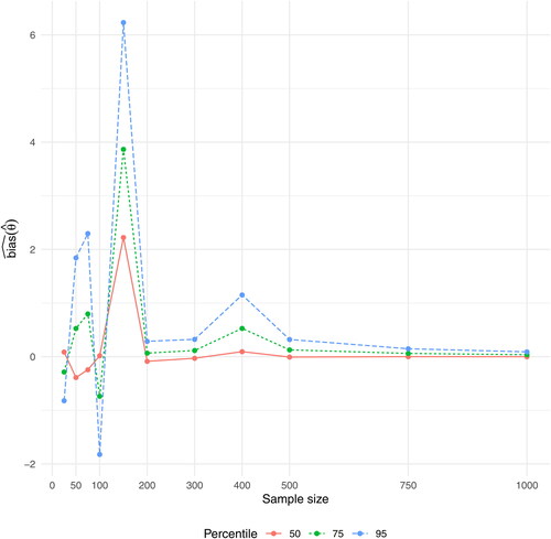
Figure 2. Graph of $\widehat{\mathit{bias}}(\widehat{\theta })$ for the case ${\beta }_3=0.5$ and ${\sigma }^2=1.$

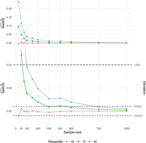
Figure 3. Graph of $\widehat{\mathit{bias}}(\widehat{\theta })$ for the case ${\beta }_3=0.9$ and ${\sigma }^2=1.$

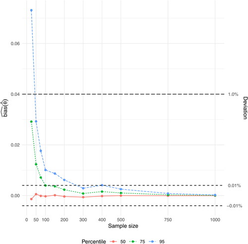
Table 2. Results of $\widehat{\mathit{bias}}(\widehat{\theta })$ for the 50th (θ = 0), 75th ($\theta =0.6744898$), and 95th ($\theta =1.644854$) percentile with ${\sigma }^2=1$ and ${\sigma }^2=4.$

		${\sigma }^2=1$			${\sigma }^2=4$
		50th	75th	95th	50th	75th	95th
β3	n	perc.	perc.	perc.	perc.	perc.	perc.
0.1	25	0.0872	−0.2850	−0.8205	1.7594	5.0535	9.7925
0.1	50	−0.3881	0.5269	1.8434	0.9437	0.7268	0.4147
0.1	75	−0.2434	0.7980	2.2962	−0.1036	−0.7137	−1.5914
0.1	100	0.0176	−0.7367	−1.8219	−0.0888	−0.3370	−0.6941
0.1	150	2.2235	3.8669	6.2310	1.2390	1.3685	1.5548
0.1	200	−0.0862	0.0668	0.2868	−0.5010	−1.3501	−2.5716
0.1	300	−0.0295	0.1152	0.3234	−0.4402	−0.8896	−1.5361
0.1	400	0.0943	0.5279	1.1516	−0.3006	0.1043	0.6868
0.1	500	−0.0071	0.1272	0.3205	−1.3287	0.8078	3.8814
0.1	750	0.0003	0.0609	0.1480	0.0114	0.2632	0.6253
0.1	1000	−0.0005	0.0366	0.0900	0.0830	0.1406	0.2234
0.5	25	−0.0041	0.0946	0.2365	0.2258	0.6895	1.3565
0.5	50	0.0023	0.0484	0.1147	0.0948	0.4322	0.9176
0.5	75	−0.0002	0.0254	0.0623	−0.1151	−1.1370	−2.6071
0.5	100	−0.0005	0.0153	0.0380	−0.0043	0.1030	0.2575
0.5	150	0.0003	0.0115	0.0276	−0.0019	0.0485	0.1210
0.5	200	−0.0006	0.0076	0.0195	−0.0011	0.0351	0.0871
0.5	300	−0.0012	0.0036	0.0105	−0.0025	0.0182	0.0481
0.5	400	−0.0003	0.0044	0.0113	−0.0007	0.0167	0.0417
0.5	500	0.0000	0.0031	0.0077	−0.0001	0.0125	0.0307
0.5	750	−0.0001	0.0014	0.0035	−0.0002	0.0067	0.0166
0.5	1000	−0.0001	0.0008	0.0019	−0.0001	0.0044	0.0109
0.9	25	−0.0014	0.0292	0.0731	0.0608	−0.0050	−0.0998
0.9	50	0.0006	0.0123	0.0293	−0.0034	0.0561	0.1417
0.9	75	−0.0001	0.0072	0.0176	−0.0002	0.0328	0.0802
0.9	100	−0.0003	0.0040	0.0101	−0.0005	0.0196	0.0486
0.9	150	0.0001	0.0036	0.0087	0.0003	0.0143	0.0345
0.9	200	−0.0004	0.0023	0.0062	−0.0007	0.0095	0.0242
0.9	300	−0.0006	0.0008	0.0029	−0.0013	0.0047	0.0132
0.9	400	−0.0002	0.0016	0.0041	−0.0004	0.0054	0.0137
0.9	500	0.0000	0.0010	0.0025	0.0000	0.0038	0.0095
0.9	750	−0.0001	0.0003	0.0008	−0.0001	0.0018	0.0045
0.9	1000	0.0000	0.0001	0.0002	−0.0001	0.0010	0.0026

Having few observations above θ should reduce the ability of $\widehat{\theta }$ to estimate θ accurately. In the present study, this is equivalent to setting θ to the 75th and 95th percentile, thus approaching the maximum value of the range of x_i. This reduced ability of $\widehat{\theta }$ to estimate θ accurately is obvious in the behavior of $\widehat{\mathit{bias}}(\widehat{\theta })$ for ${\beta }_3=0.1,$ with overall larger values of $\left|\widehat{\mathit{bias}}(\widehat{\theta })\right|$ the closer θ gets to the maximum value of the range of x_i, and with even mote pronounced volatility than for the 50th percentile (Figure 1). Thus, $\left|\widehat{\mathit{bias}}(\widehat{\theta })\right|$ has for the 75th percentile stabilized at a deviation of $<1\%$ only for n = 1000, while it for the 95th percentile never reaches this level.

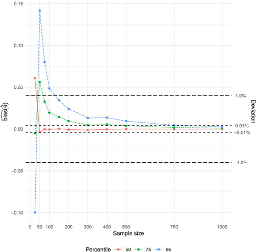
When β₃ is increasing to 0.5 and 0.9, the values of $\left|\widehat{\mathit{bias}}(\widehat{\theta })\right|$ are decreasing for all values of θ. Thus, for ${\beta }_3=0.5,$ $\left|\widehat{\mathit{bias}}(\widehat{\theta })\right|$ has for the 50th percentile stabilized at $<1\%$ already for n = 25 and has stabilized at $<0.1\%$ for n = 50, for the 75th percentile it has stabilized at $<1\%$ for n = 75 and at $<0.1\%$ for n = 500, while it for the 95th percentile has stabilized at $<1\%$ for n = 100 and at $<0.1\%$ for n = 750 (Figure 2). For ${\beta }_3=0.9,\left|\widehat{\mathit{bias}}(\widehat{\theta })\right|$ has for the 50th percentile stabilized at $<0.1\%$ already for n = 25, while it for the 75th percentile has stabilized at $<1\%$ for n = 25 and at $<0.1\%$ for n = 150, and for the 95th percentile has stabilized at $<1\%$ for n = 50 and at $<0.1\%$ for n = 500 (Figure 3).

4.2. Varying β₃ and θ for ${\sigma }^2=4$

Table 2 and Figures 4–6 give values of $\widehat{\mathit{bias}}(\widehat{\theta })$ for the case ${\sigma }^2=4$ with values of θ corresponding to the 50th, 75th, and 95th percentile of x and β₃ ranging from 0.1 to 0.9. Overall, most of the patterns observed for ${\sigma }^2=2$ are mirrored here, but with an amplified magnitude, and thus larger deviations of $\widehat{\theta }$ from the true value θ. Thus, for ${\beta }_3=0.1,\left|\widehat{\mathit{bias}}(\widehat{\theta })\right|$ has even for n = 1000 not stabilized at a deviation of $<1\%$ for any of the studied percentiles.

Figure 4. Graph of $\widehat{\mathit{bias}}(\widehat{\theta })$ for the case ${\beta }_3=0.1$ and ${\sigma }^2=4.$

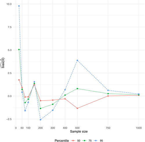
Figure 5. Graph of $\widehat{\mathit{bias}}(\widehat{\theta })$ for the case ${\beta }_3=0.5$ and ${\sigma }^2=4.$

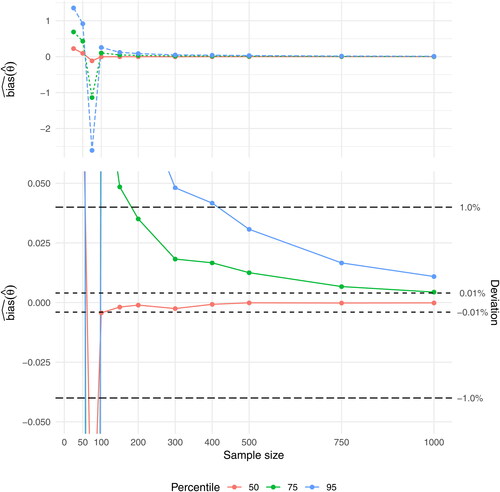
Figure 6. Graph of $\widehat{\mathit{bias}}(\widehat{\theta })$ for the case ${\beta }_3=0.9$ and ${\sigma }^2=4.$

For ${\beta }_3=0.5,\left|\widehat{\mathit{bias}}(\widehat{\theta })\right|$ has for the 50th percentile stabilized at a deviation of $<1\%$ for n = 100 and at $<0.1\%$ for n = 150, while it for the 75th percentile has stabilized at $<1\%$ for n = 200, but has not reached $<0.1\%$ even for n = 1000. For the 95th percentile, $\left|\widehat{\mathit{bias}}(\widehat{\theta })\right|$ has stabilized at a deviation of $<1\%$ for n = 500, but has not reached $<0.1\%$ for n = 1000 (Figure 5). For ${\beta }_3=0.9,\left|\widehat{\mathit{bias}}(\widehat{\theta })\right|$ has for the 50th percentile stabilized at both $<1\%$ and $<0.1\%$ for n = 50, while it for the 75th percentile has stabilized at $<1\%$ for n = 75 and at $<0.1\%$ for n = 500. For the 95th percentile, finally, has $\left|\widehat{\mathit{bias}}(\widehat{\theta })\right|$ stabilized at a deviation of $<1\%$ for n = 150 and at a deviation of $<0.1\%$ for n = 1000 (Figure 6).

5. Discussion

In this paper, we have derived an analytical formula for the expected value of the OLS based estimator $\widehat{\theta }$ of the extremum value or turning point θ in the quadratic regression model, from which formulas for the variance and bias of $\widehat{\theta }$ followed easily. Notably, the distributional assumptions for the error term ε were quite weak, not assuming that ε follows any specified distribution, such as e.g., the normal distribution. It was shown that $\widehat{\theta }$ is in general biased under these weak distributional assumptions for the error term ε, and if the normality assumption is strictly applied, neither $E(\widehat{\theta })$ nor $\mathit{Var}(\widehat{\theta })$ or $\mathit{bias}(\widehat{\theta })$ exist.

A simulation study of the performance of $\widehat{\theta }$ for small samples showed that, overall, the bias of $\widehat{\theta }$ decreases as the sample size increases. It seems safe to conclude that $\mathit{bias}(\widehat{\theta })\to 0$ as $n\to \infty .$ The bias is mainly affected by how close β₃ is to zero. However, if β₃ is reasonably far away from zero, preferably ${\beta }_3\ge 0.5,$ the bias of $\widehat{\theta }$ should be small or negligible for $n\ge 500.$ Moreover, the closer β₃ is to the median of the observed sample of the independent variable, the lower is the bias of $\widehat{\theta }$ and the faster is the bias approaching zero. In these situations, $\widehat{\theta }$ may thus be used as a reliable estimator of θ.

5.1. Topics for future research

In applied econometric and statistical analyses, the point estimate $\widehat{\theta }$ should be accompanied with a confidence interval for the extremum value θ. Moreover, there may also be interest in performing hypothesis tests regarding the value of θ. There has been some previous research on constructing approximate confidence intervals for θ using the OLS based estimator $\widehat{\theta },$ applying e.g., the delta method, the Fieller method, bootstrap methods, and the likelihood ratio interval method, see Hirschberg and Lye (2005) and Wood (2012). However, none of these methods have taken account of the bias of $\widehat{\theta }$ in estimating θ, which should be a prerequisite for constructing a reliable confidence interval for θ.

A crucial part in estimating the bias of $\widehat{\theta },$ in order to obtain unbiased estimates of θ, is to estimate the covariance term $\mathit{Cov}({\widehat{\beta }}_3,{\widehat{\beta }}_2/{\widehat{\beta }}_3)$ in (18(18) $$\mathit{bias}\left(\widehat{\theta }\right)=\frac{1}{2{\beta }_3}\times \mathit{Cov}\left({\widehat{\beta }}_3,\frac{{\widehat{\beta }}_2}{{\widehat{\beta }}_3}\right)$$(18) ). A possible approach to handle this would be to apply bootstrap methods. After obtaining unbiased estimates of θ, these may be combined with bootstrapping of (15(15) $$\begin{array}{c}Var\left(\widehat{\theta }\right)=\frac{1}{4\left[{\beta }_3^2+\mathit{Var}\left({\widehat{\beta }}_3\right)\right]}\times \left[{\beta }_2^2+\mathit{Var}\left({\widehat{\beta }}_2\right)-\mathit{Cov}\left({\widehat{\beta }}_3^2,\frac{{\widehat{\beta }}_2^2}{{\widehat{\beta }}_3^2}\right)\right]\\ -{\left[\theta +\frac{1}{2{\beta }_3}\times \mathit{Cov}\left({\widehat{\beta }}_3,\frac{{\widehat{\beta }}_2}{{\widehat{\beta }}_3}\right)\right]}^2\end{array}$$(15) ) for constructing confidence intervals for θ. It should be of interest to examine in which cases the unbiased estimates of θ obtained in this way would be outside the usual 95% confidence intervals constructed using e.g., the delta or Fieller method, i.e., how large the bias would have to be to shift the confidence intervals away from the true value of θ. Another approach would be to apply the delta method to (18(18) $$\mathit{bias}\left(\widehat{\theta }\right)=\frac{1}{2{\beta }_3}\times \mathit{Cov}\left({\widehat{\beta }}_3,\frac{{\widehat{\beta }}_2}{{\widehat{\beta }}_3}\right)$$(18) ) and (15(15) $$\begin{array}{c}Var\left(\widehat{\theta }\right)=\frac{1}{4\left[{\beta }_3^2+\mathit{Var}\left({\widehat{\beta }}_3\right)\right]}\times \left[{\beta }_2^2+\mathit{Var}\left({\widehat{\beta }}_2\right)-\mathit{Cov}\left({\widehat{\beta }}_3^2,\frac{{\widehat{\beta }}_2^2}{{\widehat{\beta }}_3^2}\right)\right]\\ -{\left[\theta +\frac{1}{2{\beta }_3}\times \mathit{Cov}\left({\widehat{\beta }}_3,\frac{{\widehat{\beta }}_2}{{\widehat{\beta }}_3}\right)\right]}^2\end{array}$$(15) ) to obtain better approximate confidence intervals. These questions will be the topics of forthcoming papers. Further topics for future research, which may be examined in simulation studies, are e.g., the bias of $\widehat{\theta }$ for other distributions of the independent variable x and the error term ε than the normal distribution, especially non-symmetric distributions such as the log-normal distribution, and the bias of $\widehat{\theta }$ when estimating the quadratic regression model (1(1) $$y={\beta }_1+{\beta }_{2}x+{\beta }_3{x}^2+\epsilon$$(1) ) using least absolute deviation (LAD) or quantile regression methods.

Finally, it should be noted that there are several econometric and statistical application areas where other functional forms for the independent variables in the linear regression model than the quadratic function in (1(1) $$y={\beta }_1+{\beta }_{2}x+{\beta }_3{x}^2+\epsilon$$(1) ) are used, and where statistical inference regarding ratios of regression coefficients are of interest. An overview of econometric applications, such as e.g., the willingness to pay value, i.e., the maximum price someone is willing to pay for a product or service, is given by Lye and Hirschberg (2018). The method for deriving analytical formulas for the expected values of estimators of ratios of regression coefficients outlined in this paper may be useful even for these cases.

Acknowledgments

The author is thankful to the anonymous reviewer for useful comments that have improved the manuscript considerably.

References

- Aghion, P., N. Bloom, R. Blundell, R. Griffith, and P. Howitt. 2005. Competition and Innovation: An Inverted-U relationship. The Quarterly Journal of Economics 120 (2):701–28. doi:10.1093/qje/120.2.701.
- Blanchflower, D. G. 2007. International Patterns of Union Membership. British Journal of Industrial Relations 45 (1):1–28. doi:10.1111/j.1467-8543.2007.00600.x.
- Blanchflower, D. G., and A. J. Oswald. 2016. Antidepressants and age: A new form of evidence for U-shaped well-being through life. Journal of Economic Behavior & Organization 127:46–58. doi:10.1016/j.jebo.2016.04.010.
- Craig, C. C. 1942. On frequency distributions of the quotient and of the product of two statistical variables. The American Mathematical Monthly 49 (1):24–32. doi:10.1080/00029890.1942.11991175.
- Dinda, S. 2004. Environmental Kuznets curve hypothesis: A survey. Ecological Economics 49 (4):431–55. doi:10.1016/j.ecolecon.2004.02.011.
- Frishman, F. 1971. On the arithmetic means and variances of products and ratios of random variables. Tech. rep. AD-785623. Durham, NC: U.S. Army Research Office.
- Frishman, F. 1975. On the arithmetic means and variances of products and ratios of random variables. In A modern course on statistical distributions in scientific work, ed. G. P. Patil, S. Kotz, and J. K. Ord, 401–6. Dordrecht: Springer Netherlands.
- Goldin, C. 1995. The U-shaped female labor force function in economic development and economic history. In Investment in women’s human capital, ed. T. Paul Schultz, Chap. 3, 61–90. Chicago: University of Chicago Press.
- Hirschberg, J. G., and J. N. Lye. 2005. Inferences for the extremum of quadratic regression models. Tech. rep. 906. Melbourne: Department of Economics, The University of Melbourne.
- Kuznets, S. 1955. Economic growth and income inequality. The American Economic Review 45 (1):1–28.
- Lye, J., and J. Hirschberg. 2018. Ratios of parameters: Some econometric examples. Australian Economic Review 51 (4):578–602. doi:10.1111/1467-8462.12300.
- Sigal, M. J., and R. P. Chalmers. 2016. Play it again: Teaching statistics with Monte Carlo simulation. Journal of Statistics Education 24 (3):136–56. doi:10.1080/10691898.2016.1246953.
- Wood, M. 2012. Bootstrapping confidence levels for hypotheses about quadratic (U-shaped) regression models. Tech. rep. Portsmouth: University of Portsmouth Business School. http://arxiv.org/abs/0912.3880v4.