Functional data clustering using principal curve methods

Abstract

In this paper we propose a novel clustering method for functional data based on the principal curve clustering approach. By this method functional data are approximated using functional principal component analysis (FPCA) and the principal curve clustering is then performed on the principal scores. The proposed method makes use of the nonparametric principal curves to summarize the features of the principal scores extracted from the original functional data, and a probabilistic model combined with Bayesian Information Criterion is employed to automatically and simultaneously find the appropriate number of features, the optimal degree of smoothing and the corresponding cluster members. The simulation studies show that the proposed method outperforms the existing functional clustering approaches considered. The capability of this method is also demonstrated by the applications in the human mortality and fertility data.

Keywords:

• Clustering
• functional data analysis
• functional principal component analysis
• principal curves

1. Introduction

In recent years functional data have received growing interests and functional data analysis (FDA) has become increasingly important in various disciplines, such as statistics, biology, economics, chemometrics, among others, due to the fast development in computing and data collection technology. Functional data is represented by a set of curves belonging to an infinite dimensional space (Ramsay and Silverman 2005; Ferraty and Vieu 2006). Under the functional data context, a curve is a random function, which is also considered as a sample from a stochastic process. Functional data analysis (FDA) refers to statistical analysis of data sets consisting of such random functions (Shang 2014). FDA can reveal more statistical information contained in the smoothness and derivatives of the functions, which distinguishes it from the multivariate data analysis (Ramsay and Silverman 2005).

Among others clustering functional data is one of the most important problems in FDA. Clustering, as an unsupervised learning process, aims at partitioning a data set into sub-groups so that the instances within a group are similar to each other while they are dissimilar to instances of other groups. Given a set of functional data, it is an interesting and valuable task to identify homogeneity and heterogeneity among curves by using the clustering techniques, which helps to unveil the potential features and patterns of the underlying stochastic processes. In the literature, a number of functional clustering methods have been developed, which can roughly be categorized into four groups: raw data clustering, filtering methods, adaptive methods, and distance-based methods (Jacques and Preda 2014). The raw data methods are to cluster directly the curves on their observed points (see, for example, Bouveyrona and Brunet-Saumard (2014)). The filtering methods first approximate the curves by basis functions or eigenfunctions and then perform clustering using the basis expansion coefficients or principal component scores: in Abraham et al. (2003) and Rossi, Conan-Guez, and El Golli (2004), the curves are approximated by the popular B-spline and then k-means and self-organized map are applied respectively to their coefficients for clustering; Peng and Müller (2008) uses the k-means algorithm on the principal component scores obtained from functional principal component analysis (FPCA). The adaptive methods are based on probabilistic models for basis expansion coefficients, FPCA scores or curves themselves: James and Sugar (2003) models the spline basis expansion of the curves especially adapted for sparsely sampled functional data and considers the coefficients to distribute according to a mixture of Gaussian distribution; Gaffney (2004) implements a family of clustering algorithms based on Gaussian mixtures combined with spline or polynomial basis approximation; Delaigle and Hall (2010) uses the density of principal components obtained from the FPCA of the curves; Bouveyron and Jacques (2011) and Jacques and Preda (2013) assume a Gaussian distribution of the principal components and define probabilistic model based clustering techniques by a mixture model; Shi and Wang (2008) models the curves directly as a mixture of Gaussian processes. Other examples of adaptive clustering include Fraley and Raftery (2002), Wakefield, Zhou, and Self (2003), and Booth, Casella, and Hobert (2008). Finally, distance-based methods adapt the conventional multivariate clustering algorithms to functional data, by defining appropriate distances or dissimilarities between curves; examples of this category include Ferraty and Vieu (2006), Tarpey and Kinateder (2003), Ieva et al. (2013). We refer to Jacques and Preda (2014) for an extensive review on the topic of functional data clustering.

In this paper we propose a new clustering method for functional data, based on the principal curve clustering approach. Principal curve is an extension of principal component and it is intuitively described as one-dimensional smooth curves that pass through the middle of a high dimensional data set. Hastie and Stuetzle (1989), which develops the fundamental framework for principal curves, defines principal curves as the self-consistent curves whose points are the average over all points that project there. Since its introduction, principal curves have been developed and applied in various fields. Banfield and Raftery (1992) implements a principal-curve method to identify the outlines of ice floe in satellite images. Stanford and Raftery (2000) constructs a principal curve clustering algorithm to detect curvilinear features in spatial point patterns. Gorban and Zinovyev (2001) presents a method for visualization of data by elastic principal manifolds. Gorban and Zinovyev (2010) analyses the nonlinear quality of life index for 171 countries by finding a principal curve that goes through a 4 D space dataset and the projections of the data points on this curve are used for ranking. Mulier and Cherkassky (1995) and Yin (2008) discuss the close connection between principal curves and self-organizing maps (SOM) which remain one of the most popular approaches for constructing approximations to the principal curves. Motivated by the above applications, we introduce the principal curve framework to the context of functional data clustering, which, to the best of our knowledge, is the first work to apply principal curve to cluster functional data. The proposed method falls into the category of filtering methods as discussed above, that is, the functional data are first approximated using functional principal component analysis and the principal curve clustering technique is then applied to the principal component scores. The proposed method makes use of the nonparametric principal curves to summarize the features of the principal scores extracted from the original functional data for clustering purpose. A probabilistic model combined with Bayesian Information Criterion (BIC) is employed to automatically and simultaneously find the appropriate number of features, the optimal degree of smoothing and the corresponding cluster members. The simulation studies show that the proposed method outperforms the existing functional clustering approaches under consideration. The capability of this method is also demonstrated by the applications in the human mortality and fertility data.

The rest of the paper is organized as follows. In Section 2, some background of functional principal component analysis (FPCA) is revisited. Section 3 briefly reviews the concept of principal curves and introduces the algorithm for clustering functional data by principal curve method. The proposed method is evaluated using simulation studies in Section 4, and two real data sets are used to illustrate its usefulness in Section 5. Finally, Section 6 concludes the paper with some discussions and possible future works.

2. Functional principal component analysis

Functional principal component analysis (FPCA) extends the classical multivariate principal component analysis by treating data as functions or curves. It is based on the fundamental theory developed independently by Karhunen (1946) and Loève (1946) about the expansion of an L₂-continuous stochastic process. Later on, Rao (1958) and Tucker (1958) applied the Karhunen-Loève (KL) expansion to functional data. In Dauxois, Pousse, and Romain (1982), some important asymptotic properties of the FPCA elements for the infinite-dimensional data were derived. Since then, there have been many theoretical developments of FPCA mainly in two streams: the linear operator point of view and the kernel operator point of view. The former includes the works by Besse (1992), Mas (2002) and Bosq (2000). And the latter relates to more recent works by Yao, Müller, and Wang (2005), Hall, Müller, and Wang (2006) and Shen (2009). Besides, some extensions and modifications of FPCA, including smoothed FPCA, sparse FPCA and multi-level FPCA, are also proposed by various researchers. In this section we briefly explain FPCA from the kernel viewpoint.

Let Y be an L₂-continuous stochastic process defined on some set $\mathcal{T}$ (time interval for instance), then: $$\forall t\in \mathcal{T},\underset{h\to 0}{\text{lim}}E\left[{\left|Y\left(t+h\right)-Y\left(t\right)\right|}^2\right]=0,$$ where $E[•]$ stands for the expectation operator. Let $\mu (t)=E{[Y(t)]}_{t\in \mathcal{T}}$ be the mean function of Y. If $L_2(\mathcal{T})$ is the space of the square-integrable functions defined on $\mathcal{T},$ then the covariance function of Y, denoted as C, is defined as: $$C\left(s,t\right)=\mathit{Cov}\left(Y\left(s\right),Y\left(t\right)\right)=E\left[\left(Y\left(s\right)-\mu \left(s\right)\right)\left(Y\left(t\right)-\mu \left(t\right)\right)\right],s,t\in \mathcal{T}.$$ And the covariance operator $\mathcal{C}$ of Y is induced by: $$\begin{array}{c}\mathcal{C}:L_2\left(\mathcal{T}\right)\to L_2\left(\mathcal{T}\right),\\ f\to \mathcal{C}f={\int }_{\mathcal{T}}C\left(•,t\right)f\left(t\right)dt.\end{array}$$ With the definition of covariance operator, one can carry out the spectral analysis of $\mathcal{C}:$ $$\mathcal{C}\varphi =l\varphi ,$$ to obtain a set of positive eigenvalues ${\left\{l_i\right\}}_{i\ge 1}$ associated with a set of orthonormal eigenfunctions ${\left\{{\varphi }_i\right\}}_{i\ge 1},$ where $l_1>l_2>\cdots \ge 0$ and ${\int }_{\mathcal{T}}{\varphi }_i(t){\varphi }_{i\prime }(t)dt=1$ if $i=i\prime$ and 0 otherwise.

Then by Karhunen-Loève (KL) expansion, the stochastic process Y can be expressed as: $$Y\left(t\right)=\mu \left(t\right)+\sum _{k=1}^{\infty }{\beta }_k{\varphi }_k\left(t\right),t\in \mathcal{T},$$ where ${\beta }_k={\int }_{\mathcal{T}}(Y(t)-\mu (t)){\varphi }_k(t)dt,k=1,2,\dots ,$ are the principal component scores. They are a sequence of uncorrelated random variables with mean zero and variance $l_k,k\ge 1.$ The principal component scores can be intuitively interpreted as the projections of the centered stochastic process ($Y(t)-\mu (t)$) in the direction of the eigenfunctions $\left\{{\varphi }_k\right\}.$ To obtain an approximation of Y(t) in L₂ norm we usually truncate the above expansion at the first N terms $$Y\left(t\right)=\mu \left(t\right)+\sum _{k=1}^N{\beta }_k{\varphi }_k\left(t\right),t\in \mathcal{T},$$ which accounts for most part of the total variation. The cumulative percentage of the overall variation explained by the first N components is given by the ratio ${\sum }_{k=1}^N{l}_k/{\sum }_{k=1}^{\infty }{l}_k.$ To have a good approximation, in this paper we require the cumulative percentage to exceed 95%, which is used to determine the optimal number of components.

In practice, the curves are observed at discrete observation points, so the principal component scores can be obtained numerically (Ramsay and Silverman 2005).

3. Principal curve clustering

3.1. Principal curves

A principal curve is a smooth, one dimensional nonparametric curve that passes through the “middle” of a p-dimensional data set. Unlike the principal component, which is linear summarization of data, a principal curve allows for nonlinearity in summarizing data and is actually an extension of the first principal component. The fundamental idea was introduced by Hastie and Stuetzle (1989) (hereafter HS), using the concept of self-consistency, which means that each point of the curve is the average over all points that project there. Assume X is a random vector in ${\mathit{R}}^p$ with density h and $f(\lambda )=(f_1(\lambda ),\dots ,f_p(\lambda ))$ is a smooth parameterized curve which does not intersect itself and has finite length inside any bounded subset of ${\mathit{R}}^p.$ The projection index ${\lambda }_f(x):{\mathit{R}}^p\to {\mathit{R}}^1$ is the function that projects points in ${\mathit{R}}^p$ orthogonally onto the curve f and is defined as: $${\lambda }_f\left(x\right)=su{p}_{\lambda }\left\{\lambda :\Vert x-f\left(\lambda \right)\Vert =in{f}_{\mu }\Vert x-f\left(\mu \right)\Vert \right\}.$$ The projection index is the largest value of λ for which $f(\lambda )$ is closest to x. Then, the curve $f(\lambda )$ is called principal curve of h if it satisfies: $$E\left(X|{\lambda }_f\left(X\right)=\lambda \right)=f(\lambda ),$$ for almost all λ.

The algorithm for finding a principal curve involves starting with the first principal component as a smooth curve and then repeating the projection and conditional expectation from the definitions above until the convergence is achieved. In practice the conditional expectation is usually replaced by a scatterplot smoother, where the conditional expectation at ${\lambda }_i$ is estimated by averaging all the observations x_k in the sample for which the corresponding ${\lambda }_k$ is close to ${\lambda }_i.$ This algorithm, motivated by the definition of finding principal curves from the sample, considers to estimate a population quantity that minimizes a population criterion. On the other hand, HS also provides an alternative algorithm to fit the principal curves by using cubic smoothing splines, which minimizes a data-dependent criterion and will be discussed in more details in next subsection. In addition to this classical definition given by HS, there exist some other definitions, such as Tibshirani (1992) and Kégl et al. (2000). Their algorithms share some common property: they all start with a straight line (very often the first principal component) and then evolve the line until it satisfactorily converges to the middle of the data. This family of algorithms is called “top-down” strategies.

Parallel to the above, “bottom-up” strategies are another family of algorithms, which, instead of starting with a global initial line, constructs the principal curve by taking into account the data in a local neighborhood of the current point considered in every step. These methods are able to handle complex data structure such as spirals or branched curves which “top-down” methods are often difficult to deal with. Delicado (2001) first introduces a principal curve approach that belongs to this family, and Einbeck, Tutz, and Evers (2005) adopts Delicado’s concept and simplifies his algorithm to be fast and efficient in computation.

In this paper the classical HS algorithm is adopted to construct principal curves for our functional clustering approach.

3.2. The spline-smoothing algorithm

Let $x_i\in {\mathit{R}}^p,i=1,\dots ,n$ be the observations of the random vector X. According to HS, the criterion for defining principal curves in this context is: find $f(\lambda )$ and ${\lambda }_i\in \left[0,1\right](i=1,\dots ,n)$ so that the penalized least squares $$D^2\left(f,{\lambda }_i\right)=\sum _{i=1}^n{\Vert x_i-f({\lambda }_i)\Vert }^2+\eta {\int }_0^1{\Vert f^{″}(\lambda )\Vert }^{2}d\lambda$$ is minimized over all functions f with $f\prime$ absolutely continuous and $f″\in L_2,$ where η is the penalty (smoothing parameter). The spline-smoothing algorithm designed on this criterion is given as follows:

1. Given f, minimizing $D^2(f,{\lambda }_i)$ over ${\lambda }_i,$ then rescale ${\lambda }_i$ to lie in $[0,1].$

2. Given ${\lambda }_i,$ split the penalized least squares into p expressions (one for each coordinate function), then smooth each coordinate separately against ${\lambda }_i$ using a cubic spline smoother with parameter η.

The smoothing parameter η controls the smoothness of the principal curve, and, as suggested by HS, can be determined by the degrees of freedom (DF) of the cubic spline which is given by the trace of the implicit smoother matrix.

3.3. Principal curve clustering for multivariate data

Stanford and Raftery (2000) proposes a clustering algorithm based on principal curves for multivariate data, which contains three main steps: denoising, initial clustering and hierarchical principal curve clustering (HPCC). The first step aims to separate the feature points from potential background or feature noise. In the second step, a model-based clustering method is used for initial clustering of the feature points. The third step, hierarchical principal curve clustering, aims to find the appropriate number of clusters and combine potential feature clusters until the desired number of clusters is reached. They uses the Bayesian Information Criterion (BIC) to determine the optimal number of clusters and introduces a clustering criterion based on a weighted sum of the squared distances about the curve (V_about) and the squared distances along the curve (V_along).

The issue with the above algorithm is that, the final step is a two-stage process, which first employs the BIC for choosing the appropriate number of final clusters and then uses the clustering criterion for step-by-step merging, which makes the algorithm very complex. Furthermore, in the clustering criterion, the weights allocated to V_about and V_along need to be chosen properly, which arouses extra difficulty in practice. In this paper we propose a slightly different probabilistic model and develop a BIC to automatically and simultaneously find the appropriate number of clusters, the optimal degree of smoothing and the corresponding cluster members.

Suppose X is a random variable in ${\mathit{R}}^p$ with a set of observations $\mathit{X}=\{x_1\dots x_n\},$ and D is a partition consisting of clusters $D_1,\dots D_M.$ It is assumed that the feature points are distributed normally along the true underlying feature. At the same time, it is also assumed that the projections of all the feature points spread uniformly along the lengths of the features’ principal curves. That is, their projections onto the corresponding principal curves form a uniform distribution $U(0,{\nu }_j),$ where ${\nu }_j$ is the length of the $j\text{th}$ curve. We also assume that the feature points are normally distributed about the true underlying feature with mean 0 and variance ${\sigma }_j^2.$ The M clusters are then modeled by a mixture model with the unconditional probability of a point belonging to the $j\text{th}$ cluster denoted by ${\pi }_j(j=1,\dots M).$

Let θ denote the entire set of parameters, then the likelihood is given by $$L\left(\mathit{X}|\theta \right)=\prod _{i=1}^{n}L(x_i|\theta ),$$ where $L(x_i|\theta )={\sum }_{j=1}^M{\pi }_{j}L(x_i|\theta ,x_i\in D_j),{\sum }_{j=1}^M{\pi }_j=1,$ and $$L\left(x_i|\theta ,x_i\in D_j\right)=\frac{1}{{\nu }_j}\left[\frac{1}{\sqrt{2\pi {\sigma }_j^2}}\text{exp}\hspace{0.17em}\left(\frac{-{\Vert x_i-f_j({\lambda }_{ij})\Vert }^2}{2{\sigma }_j^2}\right)\right],$$ where $\Vert x_i-f_j({\lambda }_{ij})\Vert$ is the Euclidean distance from the point x_i to its projection $f_j({\lambda }_{ij})$ on curve j.

Given the probabilistic model, we propose to use the BIC to determine the optimal number of features, the smoothness (i.e., DF) of the principal curves and the cluster members simultaneously. The BIC for a model with M features is defined as: $$\mathit{BIC}=2\hspace{0.17em}\text{log}\hspace{0.17em}\left(L\left(\mathit{X}|\theta \right)\right)-V\hspace{0.17em}\text{log}\hspace{0.17em}\left(n\right),$$ where $V=M(DF+2)+M-1$ is the number of parameters. (There are a total of M features, each involving two parameters ${\nu }_j$ and ${\sigma }_j,$ plus the degrees of freedom (DF); the mixing proportions ${\pi }_j$ contribute to the other M − 1 parameters.) Starting with the denoised and initially clustered data points (see Stanford and Raftery (2000) for details on these steps), we look for every possible pair of clusters to check if they can be merged, based on the BIC values. For each pair of clusters, we fit a model with two clusters and one with a single cluster to the data points, estimate the unknown parameters and calculate the BIC values within a reasonable range of DF for the one-feature and two-feature models respectively. If the maximum BIC value of one-feature model exceeds that of two-feature model by 2 or more (which indicates there is positive or strong evidence that the one-feature model is favored by the data (Kass and Raftery 1995)), then these two clusters are merged. The procedure is then continued until no more clusters can be merged. Compared with the original algorithm of Stanford and Raftery (2000), our modified clustering algorithm avoids the complexity of first determining the appropriate number of clusters and then performing step-by-step mergences based on two different criteria, and it can iteratively perform the mergence based on the BIC values and automatically arrive at the appropriate number of clusters.

3.4. Principal curve clustering for functional data

Now suppose that q samples from the stochastic process $Y(t)$ are observed and denoted by $Y_1(t),\dots ,Y_q(t).$ Then by FPCA, we have $$Y_s\left(t\right)=\mu \left(t\right)+\sum _{k=1}^N{\beta }_{s,k}{\varphi }_k\left(t\right),t\in \mathcal{T},s=1,2,\dots ,q.$$

This decomposition enables us to obtain a functional representation of the curves $Y_s(t),$ that is, the principal component scores ${\beta }_s=({\beta }_{s,1},\dots ,{\beta }_{s,N}),$ to which the principal curve clustering algorithm discussed in the previous subsection is applied.

The whole procedure of the proposed functional data clustering algorithm is summarized as follows.

1. Smooth the functional data observed at discrete points using appropriate smoothers. Our numerical experiments show that the smoothing strategy has no influence on the final clustering results and any appropriate smoothers can be used.

2. Decompose the smoothed functional data by FPCA and obtain the scores ${\beta }_s=({\beta }_{s,1},\dots ,{\beta }_{s,N}),s=1,2,\dots ,q$ of the first N principal components which make up over 95% of the total variation.

3. Remove the estimated noise points and make an initial clustering of ${\beta }_s$ into several initial clusters.

4. Seek for all possible pairs of individual clusters. For each pair, based on the probabilistic model, fit both a one-feature model and a two-feature model and calculate the BIC values within an approriate range of DF respectively.

5. Check if the maximum BIC of the one-feature model exceeds that of the two-feature model by 2 or more. If so, perform the merge. Otherwise, leave them as two individual clusters.

6. Keep merging until no more pair of individual clusters can be merged.

7. Obtain the finalized clusters of ${\beta }_s$ and then convert them back to the clusters of the functional data accordingly.

4. Simulation study

In this section two simulation studies are conducted to evaluate the proposed algorithm. The results are also compared with some of the existing functional clustering approaches in the literature.

4.1. Case one: semicircle scores

We simulate the functional data $Y_s(t)$ using $Y_s(t)=\mu (t)+{\sum }_{k=1}^2{\beta }_{s,k}{\varphi }_k(t)$ with the mean function $\mu (t)=4\hspace{0.17em}\text{sin}\hspace{0.17em}\left(\frac{\pi t}{5}\right),$ the first eigenfunction ${\varphi }_1(t)=-\hspace{0.17em}\text{cos}\hspace{0.17em}\left(\frac{\pi t}{10}\right)$ and the second eigenfunction ${\varphi }_2(t)=-\hspace{0.17em}\text{sin}\hspace{0.17em}\left(\frac{\pi t}{10}\right)$ for $0\le t\le 10.$ The FPC scores $({\beta }_{s,1},{\beta }_{s,2})$ are randomly generated by $${\beta }_{s,1}=\sqrt{1-{({\beta }_{s,2}+0.5)}^2}-0.15+0.1\epsilon ,{\beta }_{s,2}=-\sqrt{1-{({\beta }_{s,1}-0.5)}^2}+0.15+0.1\epsilon ,$$ with $\epsilon \sim N(0,1),$ so that $({\beta }_{s,1},{\beta }_{s,2})$ on 2 D plane forms two offset semicircles with added random Gaussian noises. We generate 200 FPC scores and the corresponding functional data using 100 equally spaced $t$ in the interval $[0,10],$ which are shown in Figures 1(a and b).

Figure 1. The semicircle case. (a) Bivariate plot of simulated principal component scores, with x-axis representing the first principal component scores and y-axis representing the second principal component scores, and (b) the corresponding functional data. (c) Bivariate plot of the first two principal component scores after applying FPCA on the simulated functional data. (d) Initial clustering of the scores after the removal of potential noises.

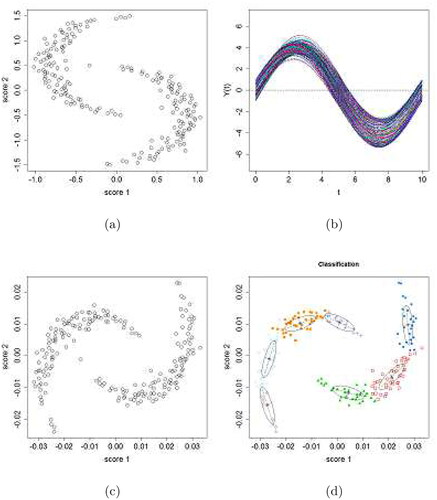
Given the sample functional data, the clustering algorithm discussed in Section 3 is then applied. The estimated functional principal component scores are obtained and shown in Figure 1(c). It is obvious that the first two principal components explain almost 100% of the total variance.

The denoising and initial clustering are conducted using k-nearest neighbor clutter removal (KNN) or robust covariance estimation by the nearest neighbor variance estimation (NNVE) and model-based clustering, respectively, and are implemented using the R package “Prabclus”, “covRobust” and “mclust”. The initial clustering results are shown in Figure 1(d).

Starting with these initial clusters, the merging process is performed iteratively for each possible pair of clusters and the BIC values are compared repeatedly to check if that pair of clusters can be merged, until no further pairs can be combined. The final clustering results are shown in Figures 2(a and b). It can be observed that the algorithm correctly identifies the two semicircles which generated the data, hence produces accurate clustering for the functional data.

Figure 2. The semicircle case. (a) Final clustering results of the scores, and (b) the corresponding clusters of the functional data. Cluster-one is in red and cluster-two in blue. The black stands for noises. (c) Final clustering results reflected by the FPCA scores produced by FunHDDC and the Curve Clustering Toolbox, and (d) those produced by the k-means method.

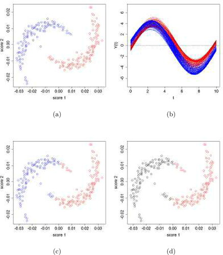
We now compare the performance of our principal curve clustering method with some other popular functional clustering methods, namely, functional k-means (Peng and Müller 2008) of the filtering methods and FunHDDC (Bouveyron and Jacques 2011) of the adaptive methods. The functional k-means clustering algorithm is to apply the k-means algorithm to the FPCA scores. It is found that the k-means algorithm identifies four clusters in the data, so fails to recognize the inherent semicircle features. The FunHDDC algorithm is based on a functional latent mixture model and the appropriate number of clusters for a dataset is determined by the BIC criterion. The implementation of the algorithm suggests six as the optimal number of clusters, which betrays the inherent feature of semicircles. We further investigate the performances of these alternative functional clustering methods by specifying the correct number of clusters as 2 and applying the k-means and FunHDDC methods to the same set of the simulated functional data. To better visualize the clustering results we plot the corresponding 2 D FPCA scores, as displayed in Figures 2(c and d). It can be observed that, even given the correct number of clusters, these two methods still cannot produce accurate classification (with the points at the end of the semicircles misclassified).

We also consider the curve clustering method developed by Gaffney (2004) using the Curve Clustering Toolbox for MATLAB. The package does not provide a means to determine the number of clusters, so we specify it as two and find the clustering results appear to be the same as that by FunHDDC.

4.2. Case two: sinusoidal scores

In the second simulation we use the same mean function and eigenfunctions as in the previous example, but the sample FPC scores $({\beta }_{s,1},{\beta }_{s,2})$ form a sinusoidal pattern with added random Gaussian noises. We generate 200 FPC scores and the corresponding functional data where the number of observations in each curve is randomly chosen from $\{10,11,\dots ,20\}$ uniformly and the values of t are generated from a uniform distribution on the interval $[0,10].$ Figures 3(a and b) demonstrate the sample scores and the corresponding functional data.

Figure 3. The sinusoidal case. (a) Bivariate plot of the simulated principal component scores, with x-axis representing the first principal component scores and y-axis representing the second principal component scores, and (b) the corresponding functional data. (c) Initial clustering of the scores after the removal of the potential noises. (d) Final clustering of the scores. One sinusoidal feature (red circles) with noises (black circles) is identified.

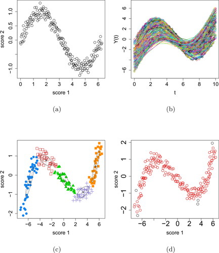
The same clustering procedure as in the case one is then conducted and the results are shown in Figures 3(c and d). Clearly the algorithm correctly recognizes the underlying sinusoidal feature of the functional data.

In this example, because the curves have different numbers of points and the values of t are also different in different curves the data cannot be treated as multivariate and k-means therefore cannot be used. Hence only the FunHDDC method is applied for comparison, which suggests the appropriate number of clusters is six. Obviously, the FunHDDC method fails to recognize the potential sinusoidal feature of the simulated functional data.

5. Empirical study

In this section, we demonstrate the capability of our principal curve clustering approach by applying it to two sets of real functional data.

5.1. French mortality

The first data set concerns the French total mortality rates from 1899 to 2012, which are obtained from the Human Mortality Database (2012). The smoothed age-specific mortality rates are represented in log scale and shown in Figure 4(a).

Figure 4. French mortality data. (a) Smoothed French total mortality rates (1899-2012). Different colors of the curves represent the mortality rates in different years. (b)-(f) Components from FPCA decomposition: the mean function, the first two functional principal components and their associated scores are displayed.

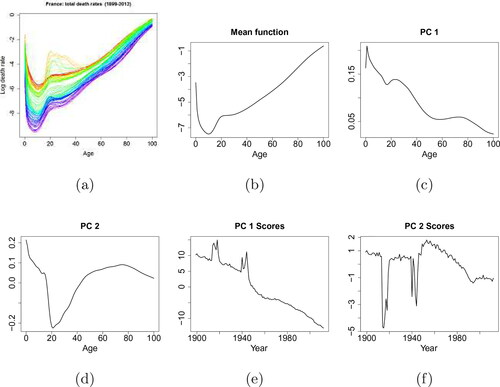
The mean function, the first two functional principal components with their corresponding principal component scores obtained by FPCA are shown in Figure 4(b–f). It is found that the first two principal components have explained 97.9% and 1.2% of the total variation respectively, hence they are adequate to represent the features of the mortality curves.

The bivariate plot of the scores is shown in Figure 5(a), with the potential noises (outliers) identified by the Robust Covariance Estimation (NNVE) method, and the initial clustering of the feature points by the model-based clustering (mclust) are demonstrated in Figure 5(b).

Figure 5. French mortality data. (a) Bivariate plot of the first two principal component scores. The red circles indicate the feature points while the blue circles indicate the potential outliers. (b) Initial clustering of the feature points after the removal of the potential noises. Four initial clusters are recognized. (c) Final clustering of the scores. Red and blue circles represent two clusters of feature points. Black circles stand for the noises. (d) Final clustering result of the French total mortality curves from 1899 to 2012 in the respective colors.

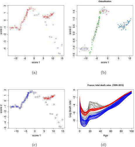
As shown in Figures 5(c and d), the final results by the clustering algorithm indicate that the left three clusters can be merged as one, while leaving the rightmost cluster as an individual one. It is obvious that the rightmost cluster of scores should be identified as a single cluster. As for the leftmost cluster, it is noticeable that there is a sharp elbow between it and its neighboring cluster. Although the merging criterion (BIC) prefers the model with one cluster more than that of two, it appears that this is a very marginal situation since the difference in their BIC values is rather small. Hence we are inclined to identify the leftmost cluster as the continuation of the previous feature, rather than considering it as the start of a new feature.

Looking into the final clustering results, the mortality curves from 1899 to 1913, 1920 to 1939 and 1941, are classified as one cluster, while those from 1949 to 2012 as the other cluster and the remaining years are identified as outliers. In fact, it can be seen from Figure 4 that the first principal component actually models the degree of variation of mortality among different age groups. The elder the age group is, the milder the variation in mortality against time it tends to have. And the decreasing trend of the first principal component scores indicates that the mortality rates are evolving lower against time. Meanwhile, the second principal component models the differences in mortality between the middle age groups and the young and old age groups. The final clustering results reflect the changes of pattern in the mortality rates in different periods. Furthermore, the outlier curves consist of two subgroups: the lower group in Figure 5(c) has extremely high mortality rates for the middle aged population and corresponds to the mortality curves of 1914–1919, 1940 and 1942–1945; the upper group situated between the two clusters refers to the mortality curves of 1946–1948. As we know, 1914–1918 is the period of WW1 while 1939–1945 is the period of WW2. France’s participation in both wars explains the unusually high mortality rates of its middle-aged population during those two periods. And the years 1946–1948 is the period right after the ending of WW2 and can be considered as a transition time to the after-war booming period.

5.2. Australian fertility

The second example is related to the age-specific Australian fertility data from 1921 to 2002. The fertility rate is defined as the number of live births during a calendar year, according to the age of the mother, per 1,000 of the female resident population of the same age at 30 June. The observed Australian fertility rates are smoothed and shown in Figure 6(a).

Figure 6. Australian fertility data. (a) Smoothed Australian fertility rates (1921-2002). Different colors of the curves represent the fertility rates in different years. (b)-(f) Components from FPCA decomposition: the mean function, the first two functional principal components and their associated scores are displayed.

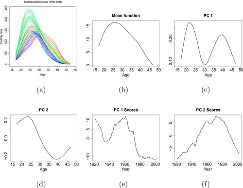
The mean function, the first two functional principal components with their corresponding principal component scores obtained by the FPCA are shown in Figures 6(b–f). The first two principal components have explained 67.9% and 28.5% of the total variation, respectively. The bivariate plot of the PC scores and the initial clustering are displayed in Figures 7(a and b). It is noted that no outliers are identified in this example. The final clustering is shown in Figures 7(c and d).

Figure 7. Australian fertility data. (a) Bivariate plot of the first two principal component scores. (b) Initial clustering of the feature points. (c) Final clustering of the scores. Red, blue and green circles represent three clusters. (d) Final clustering results of the Australian fertility curves. Red, blue and green curves correspond to clusters 1, 2 and 3 respectively.

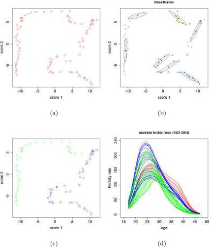
It is interesting to observe that the clustering of the Australian fertility curves actually implies a chronological order: the red curves (cluster one) represent the fertility curves from 1921 to 1930, the blue ones (cluster two) represent those from 1931 to 1963, and the green ones (cluster three) represent the remaining curves from 1964 to 2002. The result reveals some interesting trends of the evolvement of the Australian fertility rates during the past century. Cluster one curves demonstrate a generally decreasing trend of fertility over almost all age groups of women from 1921 to 1930. During that period, the peak value of fertility rate is relatively low while the fertility rates at elder ages are quite high. From 1931 to 1963, cluster two curves show a rapid increasing trend of fertility over almost all age groups of women. Meanwhile, the age groups that give highest birth rates become younger. From 1964 on to 2002, the overall fertility rates suddenly began to drop drastically with the peak value of fertility rates shifting toward higher age groups, as clearly reflected in cluster three curves. Overall, the results demonstrate that the proposed principal curve clustering method is able to detect different patterns in Australian fertility curves and consequently categorize them into appropriate groups.

6. Conclusion

In this paper we have introduced a new method for clustering functional data, based on the principal curve clustering technique. The functional data are first approximated using functional principal component analysis and the principal curve clustering technique is then applied to the principal component scores. We have improved the principal curve clustering method proposed by Stanford and Raftery (2000) and adapted it to the context of functional data. The proposed method makes use of the nonparametric principal curves to summarize the features of the principal scores extracted from the original functional data for clustering purpose. A probabilistic model combined with Bayesian Information Criterion (BIC) is developed to automatically and simultaneously find the appropriate number of features, the optimal degree of smoothing and the corresponding cluster members. In the simulation study, we demonstrate that our principal curve clustering method is capable of identifying the underlying features of the functional data, while the existing functional clustering approaches in consideration fail to do so. The capability of this method is also demonstrated by the applications to the French total mortality data and the Australian fertility data.

It can be seen that the initial clustering plays an essential role in the algorithm, since the principal curve clustering step only performs merging of the initial clusters if necessary. Therefore a larger number of initial clusters might be preferable from this point of view. However, it could be problematic in practice for two reasons: firstly more initial clusters will increase the computation time in the merging step; secondly, to fit a principal curve with reasonable smoothness each cluster would need to contain at least seven data points (as suggested by Stanford and Raftery (2000)), which restricts the number of initial clusters for a given dataset.

When deciding whether two clusters should be merged by the BIC, we assume that the principal curves fitted to each cluster have the same smoothness (DF). This assumption may not be appropriate in some cases and can be relaxed in practice. However, using different degrees of freedom for different principal curves will increase the number of candidate models significantly, which results in increased computational burden.

In this paper it is assumed that the feature points are normally distributed about the true underlying feature. Although this assumption of normality is common and reasonable in many real-life problems, it is interesting and practically useful to extend the method to other distributions.

Although the proposed method is primarily aimed for functional data, it is obvious that the algorithm can also be applied to multivariate data. In fact, the two real life examples considered in the empirical study do not fully demonstrate the advantages of functional data because the curves are observed at a small number of regular points and in this case it is expected and also confirmed by our experiments that the principal components obtained by multivariate PCA for these examples are almost the same as the FPCA components (and consequently the clustering results are the same) because the latter is an extension of the former in some sense. However, in cases where curves are observed on a dense grid, at irregular points or there exist missing values (such as the sinusoidal case in the simulation study) the multivariate data treatment can be difficult or impossible and the proposed functional data treatment will be useful. Moreover, while some functional data can also be analyzed by multivariate methods functional data treatment can still be advantageous, see for example Wang, Chen, and Xu (2017).

It is worth noting that our clustering algorithm utilizes open principal curves to identify curvilinear features underlying the functional data in order to perform clustering. However, in practice it is sometimes the case that the underlying features of functional data may scatter around a center in the space and/or display circular features, which open principal curves are unable to capture. In these cases, a clustering technique based on closed principal curves may be more suitable (Banfield and Raftery 1992).

Additional information

Funding

This work was jointly funded by the Institute and Faculty of Actuaries (IFoA) and the College of Science and Engineering of the University of Leicester (UoL) through a PhD studentship. The authors thank the editor and the reviewer for their very helpful comments.

References

- Abraham, C., P. Cornillon, E. Matzner-Løber, and N. Molinari. 2003. Unsupervised curve clustering using B-splines. Scandinavian Journal of Statistics 30 (3):581–95. doi:10.1111/1467-9469.00350.
- Banfield, J. D., and A. E. Raftery. 1992. Ice floe identification in satellite images using mathematical morphology and clustering about principal curves. Journal of the American Statistical Association 87 (417):7–16. doi:10.1080/01621459.1992.10475169.
- Besse, P. 1992. PCA stability and choice of dimensionality. Statistics & Probability Letters 13 (5):405–10. doi:10.1016/0167-7152(92)90115-L.
- Booth, J. G., G. Casella, and J. P. Hobert. 2008. Clustering using objective functions and stochastic search. Journal of the Royal Statistical Society: Series B (Statistical Methodology) 70 (1):119–39. doi:10.1111/j.1467-9868.2007.00629.x.
- Bosq, D. 2000. Linear processes in function spaces: Theory and applications. New York: Springer.
- Bouveyron, C., and J. Jacques. 2011. Model-based clustering of time series in group-specific functional subspaces. Advances in Data Analysis and Classification 5 (4):281–300. doi:10.1007/s11634-011-0095-6.
- Bouveyrona, C., and C. Brunet-Saumard. 2014. Model-based clustering of high-dimensional data: A review. Computational Statistics & Data Analysis 71:52–78.
- Dauxois, J., A. Pousse, and Y. Romain. 1982. Asymptotic theory for the principal component analysis of a vector random function: Some applications to statistical inference. Journal of Multivariate Analysis 12 (1):136–54. doi:10.1016/0047-259X(82)90088-4.
- Delaigle, A., and P. Hall. 2010. Defining probability density for a distribution of random functions. The Annals of Statistics 38 (2):1171–93. doi:10.1214/09-AOS741.
- Delicado, P. 2001. Another look at principal curves and surfaces. Journal of Multivariate Analysis 77 (1):84–116. doi:10.1006/jmva.2000.1917.
- Einbeck, J., G. Tutz, and L. Evers. 2005. Local principal curves. Statistics and Computing 15 (4):301–13. doi:10.1007/s11222-005-4073-8.
- Ferraty, F., and P. Vieu. 2006. Nonparametric functional data analysis: Theory and practice. New York: Springer.
- Fraley, C., and A. E. Raftery. 2002. Model-based clustering, discriminant analysis, and density estimation. Journal of the American Statistical Association 97 (458):611–31. doi:10.1198/016214502760047131.
- Gaffney, S. 2004. Probabilistic curve-aligned clustering and prediction with mixture models. PhD thesis., Department of Computer Science, University of California.
- Gorban, A. N., and A. Zinovyev. 2001. Visualization of data by method of elastic maps and its applications in genomics, economics and sociology. Institut des Hautes Etudes Scientifiques. Preprint. IHES M/01/36. http://cogprints.org/3082/.
- Gorban, A. N., and A. Zinovyev. 2010. Principal manifolds and graphs in practice: From molecular biology to dynamical systems. International Journal of Neural Systems 20 (3):219–32. doi:10.1142/S0129065710002383.
- Hall, P., H.-G. Müller, and J.-L. Wang. 2006. Properties of principal component methods for functional and longitudinal data analysis. The Annals of Statistics 34 (3):1493–517. doi:10.1214/009053606000000272.
- Hastie, T., and W. Stuetzle. 1989. Principal curves. Journal of the American Statistical Association 84 (406):502–16. doi:10.1080/01621459.1989.10478797.
- Human Mortality Database. 2012. Univeristy of California, Berkeley (USA), and Max Plank Institute for Demographic Research (Germany). http://www.mortality.org/.
- Ieva, F., A. Paganoni, D. Pigoli, and V. Vitelli. 2013. Multivariate functional clustering for the morphological analysis of ECG curves. Journal of the Royal Statistical Society: Series C (Applied Statistics) 62 (3):401–18. doi:10.1111/j.1467-9876.2012.01062.x.
- Jacques, J., and C. Preda. 2013. Funclust: A curves clustering method using functional random variable density approximation. Neurocomputing 112:164–71. doi:10.1016/j.neucom.2012.11.042.
- Jacques, J., and C. Preda. 2014. Functional data clustering: A survey. Advances in Data Analysis and Classification 8 (3):231–55. doi:10.1007/s11634-013-0158-y.
- James, G., and C. Sugar. 2003. Clustering for sparsely sampled functional data. Journal of the American Statistical Association 98 (462):397–408. doi:10.1198/016214503000189.
- Karhunen, K. 1946. Zur spektraltheorie stochastischer prozesse. Annales Academiae Scientiarum Fennicae 34:1–37.
- Kass, R. E., and A. E. Raftery. 1995. Bayes factors. Journal of the American Statistical Association 90 (430):773–95. doi:10.1080/01621459.1995.10476572.
- Kégl, B., A. Krzyzak, T. Linder, and K. Zeger. 2000. Learning and design of principal curves. IEEE Transactions on Pattern Analysis and Machine Intelligence 22 (3):281–97. doi:10.1109/34.841759.
- Loève, M. 1946. Fonctions aléatoires à décomposition orthogonale exponentielle. La Revue Scientifique 84:159–62.
- Mas, A. 2002. Weak convergence for the covariance operators of a Hilbertian linear process. Stochastic Processes and Their Applications 99 (1):117–35. doi:10.1016/S0304-4149(02)00087-X.
- Mulier, F., and V. Cherkassky. 1995. Self-organization as an iterative kernel smoothing process. Neural Computation 7 (6):1165–77. doi:10.1162/neco.1995.7.6.1165.
- Peng, J., and H.-G. Müller. 2008. Distance-based clustering of sparsely observed stochastic processed, with applications to online auctions. The Annals of Applied Statistics 2 (3):1056–77. doi:10.1214/08-AOAS172.
- Ramsay, J. O., and B. W. Silverman. 2005. Functional data analysis. New York: Springer.
- Rao, C. R. 1958. Some statistical methods for comparison of growth curves. Biometrics 14 (1):1–17. doi:10.2307/2527726.
- Rossi, F., B. Conan-Guez, and A. El Golli. 2004. Clustering functional data with the SOM algorithm. In Proceedings of ESANN 2004, 305–12. Bruges, Belgium.
- Shang, H. L. 2014. A survey of functional data principal component analysis. AStA Advances in Statistical Analysis 98 (2):121–42. doi:10.1007/s10182-013-0213-1.
- Shen, H. 2009. On modeling and forecasting time series of smooth curves. Technometrics 51 (3):227–38. doi:10.1198/tech.2009.08100.
- Shi, J. Q., and B. Wang. 2008. Curve prediction and clustering with mixtures of Gaussian process functional regression models. Statistics and Computing 18 (3):267–83. doi:10.1007/s11222-008-9055-1.
- Stanford, D. C., and A. E. Raftery. 2000. Finding curvilinear features in spatial point patterns: Principal curve clustering with noise. IEEE Transactions on Pattern Analysis and Machine Intelligence 22 (6):601–9. doi:10.1109/34.862198.
- Tarpey, T., and K. Kinateder. 2003. Clustering functional data. Journal of Classification 20 (1):93–114. doi:10.1007/s00357-003-0007-3.
- Tibshirani, R. 1992. Principal curves revisited. Statistics and Computing 2 (4):183–90. doi:10.1007/BF01889678.
- Tucker, L. R. 1958. Determination of parameters of a functional relation by factor analysis. Psychometrika 23 (1):19–23. doi:10.1007/BF02288975.
- Wakefield, J., C. Zhou, and S. Self. 2003. Modelling gene expression data over time: Curve clustering with informative prior distributions. Bayesian Statistics 7, 721–32.
- Wang, B., T. Chen, and A. Xu. 2017. Gaussian process regression with functional covariates and multivariate response. Chemometrics and Intelligent Laboratory Systems 163:1–6. doi:10.1016/j.chemolab.2017.02.001.
- Yao, F., H.-G. Müller, and J.-L. Wang. 2005. Functional data analysis for sparse longitudinal data. Journal of the American Statistical Association 100 (470):577–90. doi:10.1198/016214504000001745.
- Yin, H. 2008. Learning nonlinear principal manifolds by self-organising maps. In Principal manifolds for data visualization and dimension reduction, eds. A. N. Gorban, B. Kégl, D. C. Wunsch, A. Y. Zinovyev, 68–95. Lecture Notes in Computational Science and Engineering, vol. 58. Berlin, Heidelberg: Springer.