A robustness evaluation of Bayesian tests for longitudinal data

Abstract

Linear mixed models are standard models to analyze repeated measures or longitudinal data under the assumption of normality for random components in the model. Although the mixed models are often used in both frequentist and Bayesian inference, their evaluation from robustness perspective has not received as much attention in Bayesian inference as in frequentist. The aim of this study is to evaluate Bayesian tests in mixed models for their robustness to normality. We use a general class of exponential power distributions, EPD, and particularly focus on testing fixed effects in longitudinal models. The EPD class contains both light and heavy tailed distributions, with normality as a special case. Further, we consider a new paradigm of Bayesian testing decision theory where the hypotheses are formulated as a mixture model, with subsequent testing based on the posterior distribution of the mixture weights. It is shown that the EPD class provides a flexible alternative to normality assumption, particularly in the presence of outliers. Real data applications are also demonstrated.

Keywords:

• Exponential power class
• Bayesian testing
• linear mixed models
• MCMC

1. Introduction

Linear mixed models (LMM) provide standard tools to analyze longitudinal or repeated measures data in both Bayesian and frequentist inference. The LMMs offer much flexibility for modeling a variety of covariance structures and can be used for both balanced and unbalanced data. Furthermore, their implementation is facilitated through the availability of statistical software. Most of the modeling of continuous data in real life problems through LMMs is essentially based on normality assumption for the random components of the postulated model. When the assumption is not tenable, the tests and confidence intervals are no longer valid.

In Bayesian theory of LMMs, the setting of priors may have much flexibility but normality assumption is the main source of likelihood in mixed models. This leads to serious consequences for posterior modeling if the likelihood part is misspecified. The problem obviously exacerbates if the data additionally contain outliers. Such robustness aspect in Bayesian context has not been considered as often as in frequentist case, although there have been a few studies in this direction.

For example, skewness in the random components of the LMM has been considered by Arellano-Valle, Bolfarine, and Lachos (2005), Lin and Lee (2008), Zhang and Davidian (2001). Of particular interest is the study of influence of outliers using multivariate t and Laplace distributions; see e.g., Lange, Little, and Taylor (1989), Pinheiro, Liu, and Wu (2001), Rukhin and Possolo (2011), Yavuz and Arslan (2018). Another approach focuses directly on the log-likelihood by replacing the quadratic term in the normal distribution by a slower growing function (Huggins 1993).

The aforementioned references deal with a specific distribution as a replacement of normality, hence lacking a broader perspective of evaluation. Our main objective in this article is to evaluate the robustness aspect for Bayesian testing theory from the perspective of a general class of distributions, called exponential power distributions (EPD), which includes uniform, Laplace and normal distributions. The univariate EPD class was introduced by Box and Tiao (1962) for the purpose of studying robustness of Bayesian t-test; see also Box and Tiao (1964). We use its multivariate extension in the context of Bayesian testing of fixed effects in a mixed model set up for longitudinal data. The EPD class makes a subclass of elliptically contoured distributions which is widely used, particularly in frequentist inference for similar purposes.

Extension of the EPD class to the multivariate case was given in Gómez, Gomez-Viilegas, and Marín (1998). For its use as an alternative to normality in Bayesian inference, see e.g., Choy and Walker (2003), Haro-López and Smith (1999), Lindsey (1999), Walker and Gutierrex-Pena (1998). Like the normal distribution, the EPD is parametrized by location and variance parameters, but with an additional parameter which determines the kurtosis and makes the EPD class particularly attractive to study robustness. Setting this parameter to 1 reduces the EPD to normal. Otherwise, the distribution has heavier or lighter tails than normal, depending on the values of the parameter. For a special application of the EPD class in cross-over experiments, see Lindsey (1999).

The aforementioned aspect needs special emphasis in the context of Bayesian inference. Generally, the setting of priors provides most flexibility in Bayesian inference, whereas the likelihood comes from a relatively restricted assumption. If, however, the likelihood is misspecified, the resulting posterior distribution leads to seriously misleading predictive inference. Considered from this perspective, the EPD class provides alternative likelihood sources for Bayesian testing theory when normality assumption is suspect, apart from being an effective source of assessing robustness. A more technical discussion on the structure of the EPD, supplemented with graphs, is provided in Section 2.

After providing a brief orientation to the EPD class in Section 2, along with the form of mixed models to be considered under the EPD, the Bayesian framework of the problem is given in Secction 3.1, with their corresponding Markov chain Monte Carlo (MCMC) algorithms given in Section 3.2. A detailed simulation study focusing on the use of EPD for robustness in the considered models is provided in Section 3.3, where its application on real data is illustrated in Section 4.

2. Preliminaries

Consider the LMM (1) $${\mathit{y}}_i={\mathit{X}}_i\mathit{\beta }+{\mathit{Z}}_i{\mathit{b}}_i+{\mathit{e}}_i,\hspace{0.5em}i=1,\dots ,m,$$(1) where ${\mathit{y}}_i\in {\mathbb{R}}^{n_i}$ is the response vector on the ith individual, ${\mathit{X}}_i\in {\mathbb{R}}^{n_i\times p}$ and ${\mathit{Z}}_i\in {\mathbb{R}}^{n_i\times q}$ are the design matrices for the fixed and random effects respectively, with $\mathit{\beta }\in {\mathbb{R}}^p$ and ${\mathit{b}}_i\in {\mathbb{R}}^q$ the corresponding parameter vectors. We denote $N={\sum }_{i=1}^m{n}_i$ as the total number of observations. For inferential purposes, it is commonly assumed that (2) $${\mathit{b}}_i\sim {\mathcal{N}}_q(\mathbf{0},\mathbf{\Psi }),\hspace{0.5em}{\mathit{e}}_i\sim {\mathcal{N}}_{n_i}(\mathbf{0},{\sigma }^2{\mathit{I}}_{n_i}),$$(2) where $\mathbf{\Psi }\in {\mathbb{R}}^{q\times q}$ is a symmetric positive definite matrix and ${\mathit{I}}_{n_i}$ is the $n_i\times n_i$ identity matrix. $\mathbf{\Psi }$ is assumed unknown and with no specific structure. It is further assumed that ${\mathit{b}}_i$ and ${\mathit{e}}_i$ are independent.

Model (1) covers a wide variety of models as special cases. One of the simplest special cases is the one-way repeated measures ANOVA model which we shall be particularly dealing with. For this, ${\mathit{X}}_i={\mathit{Z}}_i={\mathit{1}}_{n_i}$ where ${\mathit{1}}_{n_i}$ is a $n_i\times 1$ vector of ones. To avoid confusion, the fixed and random effects under the ANOVA model shall be denoted by μ and α_i respectively. Model (1) reduces then to its one-way repeated measures ANOVA form as (3) $${\mathit{y}}_i=\mu {\mathit{1}}_{n_i}+{\alpha }_i{\mathit{1}}_{n_i}+{\mathit{e}}_i,i=1,\dots ,m.$$(3) The distributional assumptions correspondingly reduce to (4) $${\alpha }_i\sim \mathcal{N}(0,\tau ),\mathrm{ }{\mathit{e}}_i\sim {\mathcal{N}}_{n_i}(\mathbf{0},{\sigma }^2{\mathit{I}}_{n_i}),$$(4) where α_i and ${\mathit{e}}_i$ are assumed independent.

The previously outlined setting is often using in frequentist inference of Model (1) and its special form. Our purpose is to assess the tests of the fixed effects components of these models in a Bayesian context under the EPD class. The normality assumptions stated above will therefore be replaced with their counterparts under the EPD setting. For this, we provide a brief outline of the EPD class and mention some essential ingredients that will be frequently referred to in the sequel.

For a random variable y, the pdf of the univariate EPD is defined as (Box and Tiao 1962) (5) $$f(y;\mu ,\sigma ,\kappa )={\left(\sigma \Gamma (1+{(2\kappa )}^{-1})2^{1+\frac{1}{2\kappa }}\right)}^{-1}\hspace{0.17em}\text{exp}\hspace{0.17em}\left\{-\frac{1}{2}|\frac{y-\mu }{\sigma }{|}^{2\kappa }\right\},\mu \in \mathbb{R},\sigma \in {\mathbb{R}}^{+},\kappa \in {\mathbb{R}}^{+},$$(5) with mean and variance $$E(y)=\mu \text{and}\mathrm{ }\text{Var}(y)=\frac{2^{\frac{1}{\kappa }}\Gamma \left(\frac{3}{2\kappa }\right){\sigma }^2}{\Gamma \left(\frac{1}{2\kappa }\right)},$$ where κ is the kurtosis parameter, indicating the extent of non-normality. For κ = 1, (5) reduces to the normal distribution, where the distribution is leptokurtic for $\kappa <1$ and platykurtic for $\kappa >1.$

The pdf of the multivariate extension of the EPD is given as (Gómez, Gomez-Viilegas, and Marín 1998) (6) $$f(\mathit{y};\mathit{\mu },\mathbf{\Sigma },\kappa )=\frac{p\Gamma \left(\frac{p}{2}\right)}{{\pi }^{\frac{p}{2}}\Gamma (1+\frac{p}{2\beta })2^{1+\frac{p}{2\kappa }}}|\mathbf{\Sigma }{|}^{-\frac{1}{2}}\hspace{0.17em}\text{exp}\hspace{0.17em}\left\{-\frac{1}{2}{({(\mathit{y}-\mathit{\mu })}^T{\mathbf{\Sigma }}^{-1}(\mathit{y}-\mathit{\mu }))}^{\kappa }\right\},$$(6) with $$E(\mathit{y})=\mathit{\mu }\text{\hspace{0.5em}and}\mathrm{ }\text{Var}(\mathit{y})=\frac{2^{\frac{1}{\kappa }}\Gamma \left(\frac{p+2}{2\kappa }\right)}{p\Gamma \left(\frac{p}{2\kappa }\right)}\mathbf{\Sigma },$$ where $\mathit{\mu }\in {\mathbb{R}}^p$ is the mean vector, $\mathbf{\Sigma }\in {\mathbb{R}}^{p\times p}$ is the covariance matrix and $\kappa \in {\mathbb{R}}^{+}.$ We denote $\mathit{y}\sim E{P}_p(\mathit{\mu },\mathbf{\Sigma },\kappa ).$ 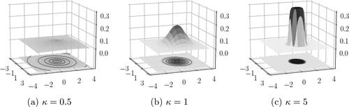Like the univariate case, the most important parameter in the multivariate EPD, particularly from the perspective of studying it as an extension to the multivariate normal distribution, is κ. Figure 1 depicts the pdf in (6) for $\kappa =\{0.5,1,5\}.$

Figure 1. The density function of $E{P}_2(\mathit{\mu },\mathbf{\Sigma },\kappa )$ displayed for $\kappa =(0.5,1,5).$ Special cases of multivariate Laplace in (a) and multivariate normal in (b).

For $\kappa \in (0,1],$ a convenient re-formulation of the multivariate EPD is in terms of scale mixture of normals (Gómez, Gómez-Villegas, and Marín 2008), as (7) $$f(\mathit{y};\mathit{\mu },\mathbf{\Sigma },\kappa )={\int }_{{\mathbb{R}}^{+}}{\mathcal{N}}_p(\mathit{y};\mathit{\mu },v^2\mathbf{\Sigma })d{H}_{\kappa }(v),$$(7) where ${\mathcal{N}}_p(·;\mathit{\mu },\mathbf{\Sigma })$ denotes a p-variate normal distribution and $H_{\kappa }$ is a one-dimensional distribution function with density function (8) $$\begin{array}{c}{h}_{\kappa }(v)=\frac{2^{1+\frac{p}{2}(1-\frac{1}{\kappa })}\Gamma (1+\frac{p}{2})}{\Gamma (1+\frac{p}{2\kappa })}{v}^{p-3}S(v^{-2};\kappa ,1,{\gamma }_{\kappa },{\delta }_{\kappa }),v>0,\\ {\gamma }_{\kappa }=2^{1-\frac{1}{\kappa }}\hspace{0.17em}\text{cos}\hspace{0.17em}\left(\pi \frac{\kappa }{2}\right),{\delta }_{\kappa }={\gamma }_{\kappa }\hspace{0.17em}\text{tan}\hspace{0.17em}\left(\frac{\pi \kappa }{2}\right),\end{array}$$(8) where $S(·;\kappa ,1,{\gamma }_{\kappa },{\delta }_{\kappa })$ in (8) is the density function of a stable distribution with characteristic function (Nolan 1997) $$\phi (t)=\hspace{0.17em}\text{exp}\hspace{0.17em}\left\{-{\gamma }_{\kappa }^{\kappa }\left|t{|}^{\kappa }\right[1-i\hspace{0.17em}\text{tan}\hspace{0.17em}\left(\frac{\pi \kappa }{2}\right)\text{sign}(t)]+i{\delta }_{\kappa }t\right\}.$$ When κ = 1, $H_{\kappa }(v)$ in (7) is degenerate at 1.

3. Bayesian tests of fixed effects under the EPD

3.1. Model set up

We are interested in evaluating the Bayesian tests for any number of the fixed effects parameters in Model (1), namely, (9) $$H_0:{({\beta }_{c_1},\dots ,{\beta }_{c_k})}^T=\mathbf{0}\text{\hspace{0.5em}vs}.\hspace{0.5em}{\mathrm{H}}_1:{({\beta }_{{\mathrm{c}}_1},\dots ,{\beta }_{{\mathrm{c}}_{\mathrm{k}}})}^{\mathrm{T}}\ne \mathbf{0},$$(9) under the EPD class, where ${\left\{c_i\right\}}_{i=1}^k\subseteq \{1,\dots ,p\}.$ The same hypotheses for the special case in (3) can be stated as (10) $$H_0:\mu =0\text{\hspace{0.5em}vs}.\hspace{0.5em}{\mathrm{H}}_1:\mu \ne 0.$$(10) To carry out these tests in a Bayesian context, we need to deal with the joint and marginal distributions of the components involved. For this, recall that we can write the distributional assumptions in (2) as (11) $$\left[\begin{array}{c}{\mathit{y}}_i\\ {\mathit{b}}_i\end{array}\right]\sim {\mathcal{N}}_{n_i+q}\left(\left[\begin{array}{c}{\mathit{X}}_i\mathit{\beta }\\ \mathbf{0}\end{array}\right],\left[\begin{array}{cc}{\mathit{Z}}_i\mathbf{\Psi }{\mathit{Z}}_i^T+{\sigma }^2{\mathit{I}}_{n_i}& {\mathit{Z}}_i\mathbf{\Psi }\\ \mathbf{\Psi }{\mathit{Z}}_i^T& \mathbf{\Psi }\end{array}\right]\right),i=1,\dots ,m.$$(11) Motivated by the procedures for robust estimation using the t-distribution outlined in Bai, Chen, and Yao (2016), Lange, Little, and Taylor (1989), Pinheiro, Liu, and Wu (2001), we recast the joint distributional assumption for EPD as (12) $$\left[\begin{array}{c}{\mathit{y}}_i\\ {\mathit{b}}_i\end{array}\right]\sim E{P}_{n_i+q}\left(\left[\begin{array}{c}{\mathit{X}}_i\mathit{\beta }\\ \mathit{0}\end{array}\right],\left[\begin{array}{cc}{\mathit{Z}}_i\mathbf{\Psi }{\mathit{Z}}_i^T+{\sigma }^2{\mathit{I}}_{n_i}& {\mathit{Z}}_i\mathbf{\Psi }\\ \mathbf{\Psi }{\mathit{Z}}_i^T& \mathbf{\Psi }\end{array}\right],\kappa \right),i=1,\dots ,m.$$(12) We shall consider the reparametrizations $\mathbf{\Psi }={\sigma }^2\mathit{D},$ where D is unknown with no assumed structure as this was assumed for $\mathbf{\Psi },$ and $\tau ={\sigma }^{2}d$ which will allow partial collapsing of the random and fixed regression coefficients in the MCMC algorithms outlined in the next section (Park and Min 2016). Thus, with the scale mixture of normal representation of the EPD, (12) can be expressed as (13) $$\left[\begin{array}{c}{\mathit{y}}_i\\ {\mathit{b}}_i\end{array}\right]\mathrm{ }|v_i\sim {\mathcal{N}}_{n_i+q}\left(\left[\begin{array}{c}{\mathit{X}}_i\mathit{\beta }\\ \mathit{0}\end{array}\right],{\sigma }^2{v}_i^2\left[\begin{array}{cc}{\mathbf{\Sigma }}_i& {\mathit{Z}}_i\mathit{D}\\ \mathit{D}{\mathit{Z}}_i^T& \mathit{D}\end{array}\right]\right),v_i\sim h_{\kappa }(v_i),$$(13) where ${\mathbf{\Sigma }}_i={\mathit{Z}}_i\mathit{D}{\mathit{Z}}_i^T+{\mathit{I}}_{n_i}.$ As interest lies in inference of the fixed effect coefficients, the marginal model of ${\mathit{y}}_i$ in (13) could be considered. This corresponds to integrating out the random effects from the posterior distribution, meaning less parameters to sample in a MCMC sampling scheme. However, this approach would lead to an unknown normalizing constant of the conditional distribution of D due to the presence of the inverse and determinant of ${\mathbf{\Sigma }}_i$ in the likelihood. Thus the joint approach is often preferred to a marginal one.

For the matrix form of (13), denote $\mathit{V}=\text{diag}(v_1,\dots ,v_m),\mathit{v}={(v_1,\dots ,v_m)}^T,$ the stacked vectors $\mathit{y}={({\mathit{y}}_1^T,\dots ,{\mathit{y}}_m^T)}^T,\mathit{b}={({\mathit{b}}_1^T,\dots ,{\mathit{b}}_m^T)}^T$ and the stacked matrices $\mathit{X}={({\mathit{X}}_1^T,\dots ,{\mathit{X}}_m^T)}^T,\mathit{Z}=\text{diag}({\mathit{Z}}_1,\dots ,{\mathit{Z}}_m)$ and $\mathbf{\Sigma }=\text{diag}(v_1{\mathbf{\Sigma }}_1,\dots ,v_m{\mathbf{\Sigma }}_m).$ Then (13) can be expressed as (14) $$\left[\begin{array}{c}\mathit{y}\\ \mathit{b}\end{array}\right]\mathrm{ }|\mathit{v}\sim {\mathcal{N}}_{N+mq}\left(\left[\begin{array}{c}\mathit{X\beta }\\ \mathit{0}\end{array}\right],{\sigma }^2\left[\begin{array}{cc}\mathbf{\Sigma }& \mathit{Z}(\mathit{V}\otimes \mathit{D})\\ (\mathit{V}\otimes \mathit{D}){\mathit{Z}}^T& (\mathit{V}\otimes \mathit{D})\end{array}\right]\right).$$(14)

Following the same strategy for the special case in (3, 13) can be expressed as (15) $$\left[\begin{array}{c}{\mathit{y}}_i\\ {\alpha }_i\end{array}\right]|v_i\sim {\mathcal{N}}_{n_i+1}\left(\left[\begin{array}{c}\mu {\mathit{1}}_{n_i}\\ 0\end{array}\right],{\sigma }^2{v}_i^2\left[\begin{array}{cc}\tilde{\mathbf{\Sigma }}& d{\mathit{1}}_{n_i}\\ d{\mathit{1}}_{n_i}^T& d\end{array}\right]\right),i=1,\dots ,m,$$(15) where ${\mathit{J}}_{n_i}={\mathit{1}}_{n_i}{\mathit{1}}_{n_i}^T$ and ${\tilde{\mathbf{\Sigma }}}_i=d{\mathit{J}}_{n_i}+{\mathit{I}}_{n_i}.$ Denote $\mathit{\alpha }={({\alpha }_1,\dots ,{\alpha }_m)}^T,$ and the block diagonal matrices $\mathit{1}=\text{diag}({\mathit{1}}_{n_1},\dots ,{\mathit{1}}_{n_m})$ and $\tilde{\mathbf{\Sigma }}=\text{diag}(v_1{\tilde{\mathbf{\Sigma }}}_1,\dots ,v_m{\tilde{\mathbf{\Sigma }}}_m).$ The matrix form of (15) is then (16) $$\left[\begin{array}{c}\mathit{y}\\ \mathit{\alpha }\end{array}\right]|\mathit{v}\sim {\mathcal{N}}_{N+m}\left(\left[\begin{array}{c}\mu {\mathit{1}}_N\\ 0\end{array}\right],{\sigma }^2\left[\begin{array}{cc}\tilde{\mathbf{\Sigma }}& d\mathit{1V}\\ d\mathit{V}{\mathit{1}}^T& d\mathit{V}\end{array}\right]\right).$$(16)

Now, under this set up, Bayesian tests of the form (9) and (10) can be carried out for which the models associated with H₀ and H₁ can be formulated as (17) $${\mathcal{M}}_0:y\sim f(y|{\theta }_0),{\theta }_0\in {\Theta }_0\mathrm{ }\text{and}\mathrm{ }{\mathcal{M}}_1:y\sim f(y|{\theta }_1),{\theta }_1\in {\Theta }_1,$$(17) respectively, with corresponding prior distributions ${\pi }_0({\theta }_0)$ and ${\pi }_1({\theta }_1).$ Further, for the hypotheses tests (9) and (10) we have ${\Theta }_0\subset {\Theta }_1.$ For example, the parameter spaces stipulated by (10) with model (16) are $${\Theta }_0={(0,\infty )}^{2+m}\times (0,1),{\Theta }_1=\mathbb{R}\times {\Theta }_0.$$ Standard procedure is then to compute the marginal likelihoods $$m_0={\int }_{{\Theta }_0}{f}_0(y|{\theta }_0){\pi }_0({\theta }_0)d{\theta }_0\mathrm{ }\text{and}\mathrm{ }{m}_1={\int }_{{\Theta }_1}{f}_1(y|{\theta }_1){\pi }_1({\theta }_1)d{\theta }_1,$$ with model choice subsequently carried out by the Bayes factor, defined as the quotient of m₀ and m₁, or the posterior probability of any of the hypotheses (Kass and Raftery 1995).

Recently, a new paradigm of Bayesian testing decision theory has been introduced. For models ${\mathcal{M}}_0$ and ${\mathcal{M}}_1$ in (17), the problem is phrased as a two component mixture (Kamary 2016) (18) $${\mathcal{M}}_{\omega }:y\sim \omega f_0(y|{\theta }_0)+(1-\omega )f_1(y|{\theta }_1),\omega \in [0,1],$$(18) with ${\pi }_0({\theta }_0)$ and ${\pi }_1({\theta }_1)$ as the corresponding priors. In this paper we use (18), where model choice is based on the posterior distribution of ω rather than a discrete choice determined by some threshold.

For hypotheses (9), the model under H₀ is considered to be nested in that under H₁, thus parametrized by the same $\mathit{\beta }.$ Let ζ₀ be a $p\times 1$ vector with zeros in the positions ${\left\{c\right\}}_{i=1}^k$ and ones in the complement ${({\left\{c\right\}}_{i=1}^k)}^c,$ where complementation is taken with respect to $\{1,\dots ,p\}.$ Denote the model matrix associated with the null hypothesis ${\mathit{X}}_{0,i}={\mathit{X}}_i\text{diag}({\zeta }_0)$ and the stacked null matrix ${\mathit{X}}_0={({\mathit{X}}_{0,1}^T,\dots ,{\mathit{X}}_{0,m}^T)}^T.$ The mixture model used for testing parts of $\mathit{\beta }$ is then (19) $${\mathcal{M}}_{\omega }^{\mathit{\beta }}:\mathit{y}\sim \omega {\mathcal{N}}_N({\mathit{X}}_0\mathit{\beta }+\mathit{Zb},{\sigma }^2\tilde{\mathit{V}})+(1-\omega ){\mathcal{N}}_N(\mathit{X\beta }+\mathit{Zb},{\sigma }^2\tilde{\mathit{V}}),$$(19) where $\tilde{\mathit{V}}=\text{diag}(v_1{\mathit{1}}_{n_1}^T,\dots ,v_m{\mathit{1}}_{n_m}^T).$ The corresponding structure for hypotheses (10) follows as (20) $${\mathcal{M}}_{\omega }^{\mu }:\mathit{y}\sim \omega {\mathcal{N}}_N(\mathit{1\alpha },{\sigma }^2\tilde{\mathit{V}})+(1-\omega ){\mathcal{N}}_N(\mu {\mathit{1}}_N+\mathit{1\alpha },{\sigma }^2\tilde{\mathit{V}}),$$(20)

After settling with the likelihood formulation, we need the priors. We consider conjugate prior distributions, conditional on the scale mixture parameters, so that the priors for the general model and its special case, (14) and (16), are, respectively, (21) $$\mu |{\sigma }^2\sim \mathcal{N}({\mu }_0,{\sigma }^2{\sigma }_{\mu }^2),\mathit{\beta }|{\sigma }^2\sim {\mathcal{N}}_p({\mathit{\mu }}_{\mathit{\beta }},{\sigma }^2{\mathbf{\Sigma }}_{\mathit{\beta }}),{\sigma }^2\sim \frac{{\sigma }_0}{{\chi }_{\nu }^2},\tau \sim \frac{{\tau }_0}{{\chi }_{\eta }^2},\mathbf{\Psi }\sim {\mathcal{W}}^{-1}(\xi ,{\mathbf{\Psi }}_0),$$(21) where ${\chi }_{\nu }^2$ denotes the ${\chi }^2$ distribution with ν degrees of freedom and ${\mathcal{W}}^{-1}(\xi ,\mathbf{\Psi })$ denotes the inverse Wishart distribution with ξ degrees of freedom and scale matrix $\mathbf{\Psi }.$ Moreover, the prior distributions of the kurtosis and mixture parameters are (22) $$\kappa \sim U(0,1)\text{\hspace{0.5em}and\hspace{0.5em}}\omega \sim \mathcal{B}\mathit{eta}(a_1,a_2).$$(22)

To sample from the posterior of (19), latent indicators $z_1,\dots ,z_m$ are utilized such that $z_i\in \{0,1\},$ with $p(z_i=0|\mathit{y},\mathit{X},\mathit{Z},{\theta }_{\mathit{\beta }}\backslash z_i)=\omega$ and $p(z_i=1|\mathit{y},\mathit{X},\mathit{Z},{\theta }_{\mathit{\beta }}\backslash z_i)=1-\omega ,$ where ${\theta }_{\mathit{\beta }}=\{\mathit{\beta },\mathit{b},\mathit{D},\mathit{z},\omega ,\mathit{v},{\sigma }^2,\kappa \}$ and $\backslash$ is the set theoretic difference. The likelihood augmented by the latent indicators is $$\begin{array}{c}p(\mathit{y},\mathit{z}|\mathit{X},\mathit{Z},{\theta }_{\mathit{\beta }}\backslash \mathit{z})=\\ \prod _{i=1}^m(\omega {\mathcal{N}}_{n_i}({\mathit{y}}_i;{\mathit{X}}_{0,i}\mathit{\beta }+\mathit{Zb},{\sigma }^2{v}_i^2{\mathit{I}}_{n_i}){)}^{z_{i0}}{((1-\omega ){\mathcal{N}}_{n_i}({\mathit{y}}_i;{\mathit{X}}_i\mathit{\beta }+\mathit{Zb},{\sigma }^2{v}_i^2{\mathit{I}}_{n_i}))}^{z_{i1}},\end{array}$$ where $z_{i0}=1_0(z_i)$ and $z_{i1}=1_1(z_i),$ where $1$ is the indicator function. Similarly, the likelihood of (20) augmented by the latent component indicators is $$p(\mathit{y},\mathit{z}|\mathit{X},\mathit{Z},{\theta }_{\mu }\backslash \mathit{z})=\prod _{i=1}^m\omega {\mathcal{N}}_{n_i}{({\mathit{y}}_i;\mathit{1\alpha },{\sigma }^2{v}_i^2{\mathit{I}}_{n_i})}^{z_{i0}}(1-\omega ){\mathcal{N}}_{n_i}{({\mathit{y}}_i;\mu \mathit{1}+\mathit{1\alpha },{\sigma }^2{v}_i^2{\mathit{I}}_{n_i})}^{z_{i1}},$$ where ${\theta }_{\mu }=\{\mu ,\mathit{\alpha },d,\mathit{z},\omega ,\mathit{v},{\sigma }^2,\kappa \}.$ The posterior distributions of (19) and (20) are thus given by (23) $$p({\theta }_{\mathit{\beta }}|\mathit{y},\mathit{X},\mathit{Z})\propto p(\mathit{y},\mathit{z}|\mathit{X},\mathit{Z},{\theta }_{\mathit{\beta }}\backslash \mathit{z})p(\mathit{b}|\mathit{y},\mathit{X},\mathit{Z},{\theta }_{\mathit{\beta }}\backslash \mathit{b})\prod _{i=1}^m{h}_{\kappa }(v_i)\pi (\mathit{\beta }|{\sigma }^2)\pi ({\sigma }^2)\pi (\mathit{D})\pi (\kappa )\pi (\omega ),$$(23) (24) $$p({\theta }_{\mu }|\mathit{y})\propto p(\mathit{y},\mathit{z}|\mathit{X},\mathit{Z},{\theta }_{\mu }\backslash \mathit{z})p(\mathit{\alpha }|\mathit{y},\mathit{X},\mathit{Z},{\theta }_{\mathit{\beta }})\prod _{i=1}^m{h}_{\kappa }(v_i)\pi (\mu |{\sigma }^2)\pi ({\sigma }^2)\pi (d)\pi (\kappa )\pi (\omega ).$$(24)

3.2. Sampling from the mixture of hypotheses

To sample from (23) we consider an extension of the partially collapsed Gibbs (PCG) sampler outlined in Park and Min (2016), based on normality and no mixture level. Outlined in Sampler 1, the MCMC sampler is designed to block $({\sigma }^2,\mathit{b},\mathit{\beta }),$ resulting in faster mixing.

Sampler 1: LMM.

Step 1: Sample ${\sigma }^2\sim p({\sigma }^2|\mathit{y},\mathit{X},\mathit{Z},{\theta }_{\mathit{\beta }}\backslash \{{\sigma }^2,\mathit{b},\mathit{\beta }\})$

Step 2: Sample $\mathit{\beta }\sim p(\mathit{\beta }|\mathit{y},\mathit{X},\mathit{Z},{\theta }_{\mathit{\beta }}\backslash \{\mathit{b},\mathit{\beta }\})$

Step 3: Sample $\mathit{b}\sim p(\mathit{b}|\mathit{y},\mathit{X},\mathit{Z},{\theta }_{\mathit{\beta }}\backslash \mathit{b})$

Step 4: Sample $\mathit{D}\sim p(\mathit{D}|\mathit{y},\mathit{X},\mathit{Z},{\theta }_{\mathit{\beta }}\backslash \mathit{D})$

Step 5: Sample $z_i\sim p(z_i|{\mathit{y}}_i,{\mathit{X}}_i,{\mathit{Z}}_i,{\theta }_{\mathit{\beta }}\backslash z_i),i=1,\dots ,m$

Step 6: Sample $\omega \sim p(\omega |\mathit{y},\mathit{X},\mathit{Z},{\theta }_{\mathit{\beta }}\backslash \omega )$

Step 7: Sample $v_i\sim p(v_i|{\mathit{y}}_i,{\mathit{X}}_i,{\mathit{Z}}_i,{\theta }_{\mathit{\beta }}\backslash v_i),i=1,\dots ,m$

Step 8: Sample $\kappa \sim p(\kappa |\mathit{y},\mathit{X},\mathit{Z},{\theta }_{\mathit{\beta }}\backslash \kappa )$

Steps 1 to 3 are a generalization of a blocked sample from $$\begin{array}{c}p({\sigma }^2,\mathit{\beta },\mathit{b}|\mathit{y},\mathit{X},\mathit{Z},{\theta }_{\mathit{\beta }}\backslash \{{\sigma }^2,\mathit{b},\mathit{\beta }\})=\\ p({\sigma }^2|\mathit{y},\mathit{X},\mathit{Z},{\theta }_{\mathit{\beta }}\backslash \{{\sigma }^2,\mathit{b},\mathit{\beta }\})p(\mathit{\beta }|\mathit{y},\mathit{X},\mathit{Z},{\theta }_{\mathit{\beta }}\backslash \{\mathit{b},\mathit{\beta }\})p(\mathit{b}|\mathit{y},\mathit{X},\mathit{Z},{\theta }_{\mathit{\beta }}\backslash \mathit{b})\end{array}$$ by partial collapsing, given that the internal order of the steps are not changed. The process of partial collapsing is achieved by marginalization, permutation and trimming (van Dyk and Park 2008). Denote ${\mathit{X}}_{i;z_i}=z_{i0}{\mathit{X}}_{0,i}+z_{i1}{\mathit{X}}_i$ and ${\mathit{X}}_{\mathit{z}}={({\mathit{X}}_{1;z_1}^T,\dots ,{\mathit{X}}_{m;z_m}^T)}^T,$ the conditional distributions of steps 1 to 3 are then given by (25) $$\begin{array}{c}{\sigma }^2|\mathit{y},\mathit{X},\mathit{Z},{\theta }_{\mathit{\beta }}\backslash \{{\sigma }^2,\mathit{b},\mathit{\beta }\}\sim (\nu {\sigma }_0^2+{(\widehat{\mathit{\beta }}-{\mathit{\mu }}_{\mathit{\beta }})}^T{\mathbf{\Sigma }}_{\mathit{\beta }}^{-1}(\widehat{\mathit{\beta }}-{\mathit{\mu }}_{\mathit{\beta }})+\text{tr}({\mathit{D}}^{-1}{\Psi }_0)+\\ {(\mathit{y}-{\mathit{X}}_z\widehat{\mathit{\beta }})}^T{\mathbf{\Sigma }}^{-1}(\mathit{y}-{\mathit{X}}_z\widehat{\mathit{\beta }}))\frac{1}{{\chi }_{\nu +N+q\eta }^2},\end{array}$$(25) (26) $$\mathit{\beta }|\mathit{y},\mathit{X},\mathit{Z},{\theta }_{\mathit{\beta }}\backslash \{\mathit{b},\mathit{\beta }\}\sim {\mathcal{N}}_p\left(\widehat{\mathit{\beta }},{\sigma }^2{({\mathbf{\Sigma }}_{\mathit{\beta }}^{-1}+{\mathit{X}}_z^T\mathbf{\Sigma }{\mathit{X}}_z)}^{-1}\right),$$(26) (27) $$\mathit{b}|\mathit{y},\mathit{X},\mathit{Y},{\theta }_{\mathit{\beta }}\backslash b\sim {\mathcal{N}}_{mq}(\widehat{\mathit{b}},{\sigma }^2(\mathit{D}-(\mathit{V}\otimes \mathit{D}){\mathit{Z}}^T{\mathbf{\Sigma }}^{-1}\mathit{Z}(\mathit{V}\otimes \mathit{D}))),$$(27) where $$\widehat{\mathit{\beta }}={({\mathbf{\Sigma }}_{\mathit{\beta }}^{-1}+{\mathit{X}}_z^T{\mathbf{\Sigma }}^{-1}{\mathit{X}}_z)}^{-1}({\mathbf{\Sigma }}_{\mathit{\beta }}^{-1}{\mathit{\mu }}_{\mathit{\beta }}+{\mathit{X}}_z^T\mathbf{\Sigma }\mathit{y}),\hspace{1em}\widehat{\mathit{b}}=(\mathit{V}\otimes \mathit{D}){\mathit{Z}}^T{\mathbf{\Sigma }}^{-1}(\mathit{y}-{\mathit{X}}_z\mathit{\beta }).$$ The conditional distribution of steps 4 to 6 are given by (28) $$\mathit{D}|\mathit{y},\mathit{X},\mathit{Z},{\theta }_{\mathit{\beta }}\backslash \mathit{D}\sim {\mathcal{W}}^{-1}\left(\eta +m,{\sigma }^{-2}({\Psi }_0+\mathit{b}{\mathit{b}}^T)\right)$$(28) (29) $$z_i|{\mathcal{X}}_i,{\theta }_{\beta }\backslash z_i\sim \mathcal{B}er\left({(1+\frac{\omega {\mathcal{N}}_{n_i}(y_i;{\mathit{X}}_{i,0}\mathit{\beta }+{\mathit{Z}}_i{\mathit{b}}_i,{\sigma }^2{v}_i^2{\mathit{I}}_{n_i})}{(1-\omega ){\mathcal{N}}_{n_i}(y_i;\mathit{X\beta }+{\mathit{Z}}_i{\mathit{b}}_i,{\sigma }^2{v}_i^2{\mathit{I}}_{n_i})})}^{-1}\right),$$(29) (30) $$\omega |\mathit{y},{\theta }_{\mathit{\beta }}\backslash \omega \sim \mathcal{B}\mathit{eta}(a_0+\sum _{i=1}^m{z}_{i1},a_1+\sum _{i=1}^m{z}_{i0}),$$(30) where $\mathcal{B}er(p)$ denotes the Bernoulli distribution with mean p. Note that the specification of (19) means that values ω closer to 1 implies that the H₀ is more likely and vice versa, as can be seen in (30).

The conditional distribution of v_i is given by (31) $$p(v_i|{\mathit{y}}_i,{\mathit{X}}_i,{\mathit{Z}}_i,{\theta }_{\mathit{\beta }}\backslash v_i)\propto h_{\kappa }(v_i){\mathcal{N}}_{n_i}({\mathit{y}}_i;{\mathit{X}}_{i;z_i}\mathit{\beta }+{\mathit{Z}}_i{\mathit{b}}_i,v_i^2{\sigma }^2{\mathit{I}}_{n_i}),$$(31) which does not have a known normalizing constant, so it is sampled by MH. As in (Gómez, Gómez-Villegas, and Marín 2008), we utilize the transformation $w_i=2^{\frac{1}{\kappa }-1}{v}_i^{-2}$ which has the conditional distribution (32) $$p(w_i|{\mathit{y}}_i,{\mathit{X}}_i,{\mathit{Z}}_i,{\theta }_{\mathit{\beta }}\backslash v_i)\propto w_i^{-\frac{n_i}{2}}S(w_i;\kappa ,1,{\gamma }_{\kappa }^{*},1,{\delta }_{\kappa }^{*}){\mathcal{N}}_{n_i}({\mathit{y}}_i;{\mathit{X}}_{i;z_i}\mathit{\beta },2^{1-\frac{1}{\kappa }}{w}_i^{-1}{\mathbf{\Sigma }}_i),$$(32) where ${\gamma }_{\kappa }^{*}=\hspace{0.17em}\text{cos}\hspace{0.17em}\left(\frac{\pi \kappa }{2}\right)$ and ${\delta }_{\kappa }^{*}={\gamma }_{\kappa }^{*}\hspace{0.17em}\text{tan}\hspace{0.17em}\left(\frac{\pi \kappa }{2}\right).$ By generating proposals independently from the previous state as $w\prime \sim S(w;\kappa ,1,{\gamma }_{\kappa }^{*},1,{\delta }_{\kappa }^{*}),$ the stable densities cancel out in the acceptance probability, given by (33) $$\psi (w_i,w\prime )=\min (1,\hspace{0.17em}\text{exp}\hspace{0.17em}\{\frac{w_i-w{\prime }_i}{2{\sigma }^2}({({\mathit{y}}_i-{\mathit{X}}_{i;z_i}\mathit{\beta }-{\mathit{Z}}_i{\mathit{b}}_i)}^T({\mathit{y}}_i-{\mathit{X}}_{i;z_i}\mathit{\beta }-{\mathit{Z}}_i{\mathit{b}}_i))\}).$$(33) The conditional density of the kurtosis parameter is given by (34) $$p(\kappa |{\theta }_{\mathit{\beta }})\propto \prod _{i=1}^m\frac{2^{1+\frac{n_i}{2}(1-\frac{1}{\kappa })}\Gamma (1+\frac{n_i}{2})}{\Gamma (1+\frac{n_i}{2\kappa })}{v}_i^{n_i-3}S(v_i^{-2};\kappa ,1,{\gamma }_{\kappa },{\delta }_{\kappa }),$$(34) where ${\gamma }_{\kappa }$ and ${\delta }_{\kappa }$ are defined as in (8). The normalizing constant of (34) is not known and κ is thus sampled by an MH-step with proposals generated by a normal random walk truncated to $[0,1]$ with standard error ϵ. The acceptance probability of proposed $\kappa \prime$ is given by (35) $$\psi (\kappa ,\kappa \prime )=\frac{p(\kappa \prime |{\theta }_{\mu }\backslash \kappa )(\Phi \left(\frac{1-\kappa }{ϵ}\right)-\Phi \left(\frac{-\kappa }{ϵ}\right))}{p(\kappa |{\theta }_{\mu }\backslash \kappa )(\Phi \left(\frac{1-\kappa \prime }{ϵ}\right)-\Phi \left(\frac{-\kappa \prime }{ϵ}\right))},$$(35) where $\Phi$ denotes the standard normal cumulative distribution function. The conditional distribution (34) is uni-modal and very peaked around its mode. A slice sampler is more suitable but leads to extreme time consumption due to repeated evaluations of the stable density function. A MH step has proved sufficient in our applications and has been compared with a slice sampler. The peakedness of (34) leads to posterior samples of κ being largely determined by the likelihood rather than the prior distribution. Replacing the uniform prior by a more informative one has little impact on the posterior distribution. Mitigating this by a truncated prior generally leads to a situation similar to fixing the kurtosis parameter at either the upper or lower bound of the truncation set.

A similar MCMC algorithm for the posterior distribution of the one-way ANOVA in (24) is outlined in Sampler 2.

Sampler 2: one-way-ANOVA.

Step 1: Sample ${\sigma }^2\sim p({\sigma }^2|\mathit{y},{\theta }_{\mu }\backslash \{{\sigma }^2,\mathit{\alpha },\mu \})$

Step 2: Sample $\mu \sim p(\mu |\mathit{y},{\theta }_{\mu }\backslash \{\mathit{\alpha },\mu \})$

Step 3: Sample $\mathit{\alpha }\sim p(\mathit{\alpha }|\mathit{y},{\theta }_{\mu }\backslash \mathit{\alpha })$

Step 4: Sample $d\sim p(d|\mathit{y},{\theta }_{\mu }\backslash d)$

Step 5: Sample $z_i\sim p(z_i|{\mathit{y}}_i,{\theta }_{\mu }\backslash z_i),i=1,\dots ,m$

Step 6: Sample $\omega \sim p(\omega |\mathit{y},{\theta }_{\mu }\backslash \omega )$

Step 7: Sample $v_i\sim p(v_i|{\mathit{y}}_i,{\theta }_{\mu }\backslash v_i),i=1,\dots ,m$

Step 8: Sample $\kappa \sim p(\kappa |\mathit{y},{\theta }_{\mu }\backslash \kappa )$

As for Sampler 1, steps 1, 2 and 3 form a blocked sample from $(\mu ,\mathit{\alpha },{\sigma }^2)$ through partial collapsing, given that their internal order is unchanged. Their conditional distributions are (36) $$\begin{array}{c}{\sigma }^2|\mathit{y},{\theta }_{\mu }\backslash \{\mu ,\mathit{\alpha }\}\sim \\ \mathrm{\hspace{1em}}\mathrm{\hspace{1em}}\frac{1}{{\chi }_{N+\eta +\nu }^2}(d^{-1}\eta {\tau }_0+\nu {\sigma }_0+\frac{{({\mu }_0-\tilde{\mu })}^2}{{\sigma }_{\mu }^2}+\sum _{i=1}^m{({\mathit{y}}_i-\tilde{\mu }{z}_{i1}{\mathit{1}}_{n_i})}^T{(v_i^2{\tilde{\mathbf{\Sigma }}}_i)}^{-1}({\mathit{y}}_i-\tilde{\mu }{z}_{i1}{\mathit{1}}_{n_i})),\end{array}$$(36) (37) $$\mu |\mathit{y},{\theta }_{\mu }\backslash \{\mu ,\mathit{\alpha }\}\sim \mathcal{N}(\tilde{\mu },{\sigma }^2{(\sum _{i=1}^m{z}_{i1}{\mathit{1}}_{n_i}^T{(v_i^2{\tilde{\mathbf{\Sigma }}}_i)}^{-1}{\mathit{1}}_{n_i}+{\sigma }_{\mu }^{-2})}^{-1}),$$(37) (38) $$\mathit{\alpha }|\mathit{y},{\theta }_{\mu }\backslash \mathit{\alpha }\sim {\mathcal{N}}_q(d\mathit{V}{\mathit{1}}^T{\tilde{\mathbf{\Sigma }}}^{-1}(\mathit{y}-\mathit{1}\mu ),d\mathit{V}-d^2\mathit{V}{\mathit{1}}^T{\tilde{\mathbf{\Sigma }}}^{-1}\mathit{1V})$$(38) where $$\tilde{\mu }={(\sum _{i=1}^m{z}_{i1}{\mathit{1}}_{n_i}^T{(v_i^2{\tilde{\mathbf{\Sigma }}}_i)}^{-1}{\mathit{1}}_{n_i}+{\sigma }_{\mu }^{-2})}^{-1}(\sum _{i=1}^m{z}_{i1}{\mathit{1}}_{n_i}^T{(v_i^2{\tilde{\mathbf{\Sigma }}}_i)}^{-1}{\mathit{y}}_i+{\sigma }_{\mu }^{-2}{\mu }_0).$$ Furthermore, ${\tilde{\mathbf{\Sigma }}}_i^{-1}={\mathit{I}}_{n_i}-{\mathit{1}}_{n_i}{\mathit{1}}_{n_i}^T\frac{d}{1+n_{i}d}$ as ${\tilde{\mathbf{\Sigma }}}_i$ is compound symmetric. The derivation of (36, 37) and (38) are outlined in the Appendix.

The conditional distributions of d, z_i and ω are given by (39) $$d|\mathit{y},{\theta }_{\mu }\backslash d\sim {\sigma }^{-2}({\tau }_0+{\mathit{\alpha }}^T\mathit{\alpha })\frac{1}{{\chi }_{\eta +m}^2},$$(39) (40) $$z_i|\mathit{y},{\theta }_{\mu }\backslash z_i\sim \mathcal{B}er\left({(1+\frac{\omega {\mathcal{N}}_{n_i}(y_i;{\alpha }_i{\mathit{1}}_{n_i},{\sigma }^2{v}_i^2{\mathit{I}}_{n_i})}{(1-\omega ){\mathcal{N}}_{n_i}(y_i;(\mu +{\alpha }_i){\mathit{1}}_{n_i},{\sigma }^2{v}_i^2{\mathit{I}}_{n_i})})}^{-1}\right),$$(40) (41) $$\omega |\mathit{y},{\theta }_{\mu }\backslash \omega \sim \mathcal{B}\mathit{eta}(a_0+\sum _{i=1}^m{z}_{i1},a_1+\sum _{i=1}^m{z}_{i0}).$$(41)

The scale mixture weight is sampled by the same procedure as in Sampler 1, with acceptance probability (42) $$\psi (w_i,w_i^{\prime })=\min (1,\hspace{0.17em}\text{exp}\hspace{0.17em}\{\frac{w_i-w{\prime }_i}{2{\sigma }^2}{({\mathit{y}}_i-{\mathit{1}}_{n_i}({\alpha }_i+z_{i1}\mu ))}^T({\mathit{y}}_i-{\mathit{1}}_{n_i}({\alpha }_i+z_{i1}\mu ))\}).$$(42)

The kurtosis parameter is sampled as in Sampler 1, with acceptance probability (35).

3.3. Simulation study

To compare performance of the mixture test for varying values of the kurtosis parameter, we consider settings similar to Pinheiro, Liu, and Wu (2001); Yavuz and Arslan (2018) with focus on the LMM and its mixture representation in (19). The kurtosis parameter is treated as a hyper-parameter by considering one-point distributions as prior distributions. Data is simulated as (43) $${\mathit{y}}_i={\mathit{X}}_i\mathit{\beta }+{\mathit{1}}_4{b}_i+{\mathit{e}}_i,\hspace{0.5em}i=1,\dots ,20.$$(43) where ${\mathit{X}}_i$ and $\mathit{\beta }$ are defined as $${\mathit{X}}_i={\left[\begin{array}{cccc}1& 1& 1& 1\\ 8& 10& 12& 14\end{array}\right]}^T\mathrm{ }\text{and}\mathrm{ }\mathit{\beta }=\left[\begin{array}{c}20\\ 0.5\end{array}\right],$$ where the null hypothesis is for the second element of $\mathit{\beta }$ being 0. The random effects and error in (43) are distributed as $$b_i\stackrel{\mathit{iid}}{\sim }\mathcal{N}(0,{\sigma }^{2}d),{\mathit{e}}_i\stackrel{\mathit{iid}}{\sim }{\mathcal{N}}_4(\mathit{0},{\sigma }^2{\mathit{I}}_4).$$ To contaminate the data with outliers, b_i and ${\mathit{e}}_i$ are expressed as mixtures $$b_i\sim (1-p_b)\mathcal{N}(0,{\sigma }^{2}d)+p_{b}f\mathcal{N}(0,{\sigma }^{2}d),\hspace{1em}{\mathit{e}}_i\sim (1-p_e){\mathcal{N}}_4(\mathit{0},{\sigma }^2{\mathit{I}}_4)+p_{e}f{\mathcal{N}}_4(\mathit{0},{\sigma }^2{\mathit{I}}_4),$$ where f is a constant used to adjust the variance of one of the components. The resulting covariance of ${\mathit{y}}_i$ is $$\text{Var}({\mathit{y}}_i)={\sigma }^2((1+(f^2-1)p_b){\mathit{J}}_4+(1+(f^2-1)p_e){\mathit{I}}_4).$$

Results are based on 500 Monte Carlo simulations for all combinations of $f=(2,4,6),\kappa =(0.6,0.7,0.8,0.9,1),$ and $p_e=(0,0.1,0.2)$ with p_b = 0, as well as a worst case scenario with $p_b=0.2,$ f = 6 and $p_e=0.2$ for all κ. We estimate the mixture weight by the posterior median based on 10⁴ samples from Sampler 1, with a transient phase of 10³ iterations. The median is considered rather than the mean as ω generally concentrates on its boundaries (Kamary 2016). The hyper-parameters are set as $$\mathit{\beta }|{\sigma }^2\sim {\mathcal{N}}_2(\mathit{0},N{\sigma }^2{({\mathit{X}}^T\mathit{X})}^{-1}),d\sim \frac{1}{{\chi }_1^2},\sigma \sim \frac{1}{{\chi }_1^2}\mathrm{ }\text{and}\mathrm{ }\omega \sim \mathcal{B}\mathit{eta}(0.5,0.5).$$

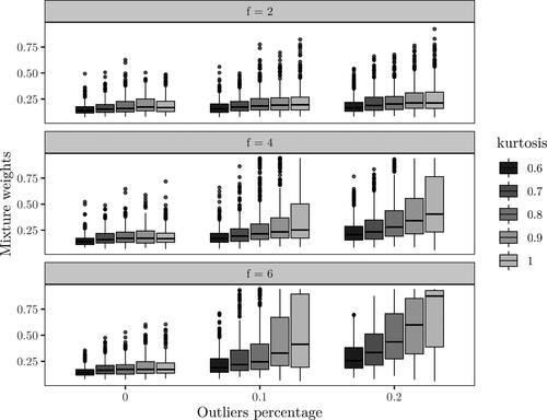
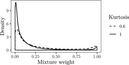
The results with no outliers in the random effects are shown in Figure 3. The effect of the kurtosis on the posterior median of the mixture weight is negligible for scaling factor f = 2. For scaling factors 4 and 6, the effect over increasing percentage of outliers is more clear. With a higher kurtosis, i.e., closer to the normal distribution, choosing the correct model gets less probable as p_e increases. The difference is most clear with scaling factor 6, where the effect of increasing p_e is quite small for $\kappa =0.6,$ but drastic for κ = 1. 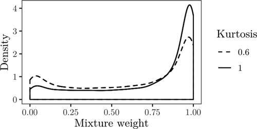The results with $p_b=p_e=0.2$ and f = 6 are displayed in Figure 2, which are nearly identical to the setting p_b = 0 and f = 6. Overall, from Figures 2 and 3, we see that inference based on lower kurtosis is less affected by increased impairment from outliers. Further, with no or low contamination by outliers, there is little difference in model choice for the different values of kurtosis.

Figure 2. Posterior median of the mixture weight for each κ with $p_e=0.2,p_b=0.2$ and f = 6.

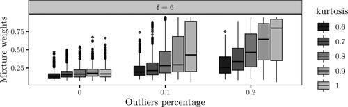
Figure 3. Posterior median of the mixture weight for each combination of κ, p_e and f with p_b = 0.

3.4. Applications

3.4.1. Example I

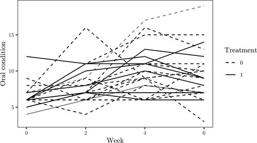
The dataset found in (Mid-Michigan Medical Center 1999) consists of repeated measurements of oral condition for 23 cancer patients. Each patient is randomly assigned to a treatment and placebo group, where the treated received aloe juice treatment. For each individual, an initial measure is taken with repeated measurements at weeks 2, 4 and 6. Other variables are initial age, weight and cancer stage of the patients. The data is displayed in Figure 4.

Figure 4. Cancer data.

The model of interest is defined as (44) $$\begin{array}{c}{y}_{ij}={\beta }_0+b_{1,i}+({\beta }_1+b_{2,i}){\text{week}}_{ij}+{\beta }_2{\text{treatment}}_i+{\beta }_3{\text{age}}_i+{\beta }_4{\text{weight}}_i+e_{ij},\\ i=1,\dots ,23j=1,\dots ,4,\end{array}$$(44) where cancer stage has been omitted as its inclusion led to issues in frequentist estimation of the random effects covariance matrix, this did not impact the results in terms of model choice. For testing parts of (44), we consider the null $H_0\text{:}\mathrm{ }({\beta }_1,{\beta }_2)\prime =\mathit{0}$ against $H_1\text{:}\mathrm{ }({\beta }_1,{\beta }_2)\prime \ne \mathit{0}.$ The hyper-parameters are set as $$\mathit{\beta }|{\sigma }^2\sim {\mathcal{N}}_5(\mathit{0},{\sigma }_{\beta }^2{\mathit{I}}_5),\mathit{D}\sim {\mathcal{W}}^{-1}(2,{\mathit{I}}_2),{\sigma }^2\sim \frac{1}{{\chi }_1^2},\omega \sim \mathcal{B}\mathit{eta}(\frac{1}{2},\frac{1}{2})\mathrm{ }\text{and}\mathrm{ }\kappa \sim U(0,1),$$ where results shall be compared for ${\sigma }_{\beta }^2=100$ and 10. All results are based on 10⁴ iterations of Sampler 1, with a burn-in phase of $5\times {10}^3$ iterations. The trace and posterior densities of the mixture weight are displayed in Figure 5, where the posterior median is estimated as 0.986 for ${\sigma }_{\beta }^2=100$ and 0.934 for ${\sigma }_2^{\beta }=10.$ The null is therefore favored with both settings of ${\sigma }_{\beta }^2,$ but the difference is quite large based on Figure 5 with much fewer jumps between models for ${\sigma }_{\beta }^2=100.$ 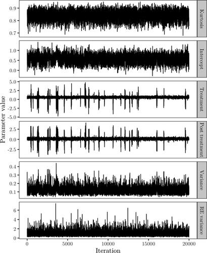Posterior samples of the kurtosis, treatment and week fixed effect coefficients and between subject variance are displayed in Figure 6. The posterior mean of the kurtosis parameter is estimated as 0.91 for both values of ${\sigma }_{\beta }^2,$ and this result is not sensitive to changes in the hyper-parameters of the prior on κ. Both the treatment and week coefficients are generally sampled by the prior with ${\sigma }_{\beta }^2=100.$ For ${\sigma }_{\beta }^2=10,$ the posterior mean of the treatment and week coefficient, based on the iterations where one or more observations are assigned to the mixture component corresponding to the alternative hypothesis, are estimated as −0.406 and 0.61 respectively. For the between subjects variance, ${\sigma }^2,$ the posterior mean with ${\sigma }_{\beta }^2=100$ and ${\sigma }_{\beta }^2=10$ are estimated as 8.72 and 8.02 respectively. The increased oscillation of the mixture weights with ${\sigma }_{\beta }^2=10$ can also be seen in the trace plots of the variance term in Figure 6, when comparing with the higher value of ${\sigma }_{\beta }^2.$ The posterior mean of the elements of D for ${\sigma }_{\beta }^2=10$ and ${\sigma }_{\beta }^2=100$ are estimated as $${\widehat{\mathit{D}}}_{{\sigma }_{\beta }^2=100}=\left[\begin{array}{cc}0.112& -0.016\\ -0.016& 0.053\end{array}\right],{\widehat{\mathit{D}}}_{{\sigma }_{\beta }^2=10}=\left[\begin{array}{cc}0.118& -0.014\\ -0.014& 0.052\end{array}\right],$$ and are thus unaffected by the increased assignment of observations to the alternative hypothesis component with ${\sigma }_{\beta }^2=10.$ In Figure 7, the random effects, e.g., $b_{1,i}$ and $b_{2,i}$ in (44), are compared for patients with Id’s 6 and 14, which are marked as gray lines in Figure 4. Patient 6 did receive treatment and thus corresponds to the dashed gray line, whilst patient 14 did not and thus correspond to the solid gray line. There is not much difference between the posterior samples for different ${\sigma }_{\beta }^2$ of the random effects.

Figure 5. Posterior sample of the mixture weight for the hypotheses of no treatment effect.

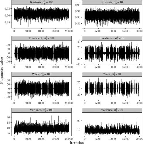
Figure 6. Trace plots of the kurtosis parameter, treatment and week fixed effect coefficients, error variance and elements of the random effects covariance based on Sampler 1.

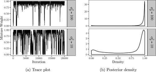
Figure 7. Posterior samples of the random effects of individuals with id 6 and 14.

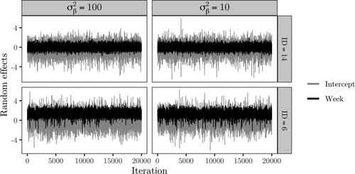
Figure 8. Posterior density of the mixture weights with the kurtosis parameter treated as a hyper-parameter.

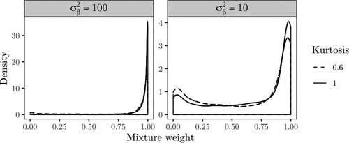
In Figure 8, the posterior density of the mixture weights are compared when fixing the kurtosis parameter to 0.6 and 1. In all settings, the null is favored. The evidence for the null is slightly weaker with a lower kurtosis for both ${\sigma }_{\beta }^2=10$ and 100.

To compare the models in a frequentist setting based on the normal likelihood, the models stipulated by the null and alternative hypotheses are estimated using the lme4 (Bates et al. 2015) package in R (R Core Team 2020) and compared using the Akaike information criterion (AIC). The AIC is 436.15 for the unrestricted model (44), where the treatment and week fixed effects are estimated as −0.622 and 0.535 respectively. The AIC for the restricted model is 444.69. Thus, the model under the alternative hypothesis is favored in a standard frequentist setting.

3.4.2. Example II

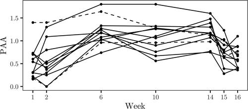
The dataset considered in Example 3.3 in Crowder and Hand (1990) consists of measurements of plasma ascorbic acid (PAA) for twelve patients that underwent dietary regime treatment with measurements taken at weeks 1, 2, 6, 10, 14, 15 and 16. First 2 weeks consist of pretreatment measurements, last 2 consists of post-treatment measurements and the measurements in the remaining weeks were taken during treatment. The data are displayed in Figure 9.

Figure 9. PAA data.

To test whether the mean for pretreatment, treatment and post-treatment are equal, the data is transformed by taking the mean within the treatment periods. Letting ${\tilde{\mathit{y}}}_i$ be the vector of 7 measurements for patient i, the data is transformed as $${\mathit{y}}_i=\left(\begin{array}{ccccccc}\frac{1}{2}& \frac{1}{2}& 0& 0& 0& 0& 0\\ 0& 0& \frac{1}{3}& \frac{1}{3}& \frac{1}{3}& 0& 0\\ 0& 0& 0& 0& 0& \frac{1}{2}& \frac{1}{2}\end{array}\right){\tilde{\mathit{y}}}_i,i=1,\dots ,12,$$ with the model specified as (45) $$y_{ij}={\mu }_j+{\alpha }_i+e_{ij},i=1,\dots ,12,j=1,2,3,$$(45) where μ_j represents the average within the ${\mathrm{j}}^{\text{th}}$ period. We shall first consider testing $H_0\text{:}\mathrm{ }{\mu }_1={\mu }_2={\mu }_3$ vs. H₁: not H₀, and subsequently $H_0\text{:}\mathrm{ }{\mu }_1={\mu }_3$ vs. $H_1\text{:}\mathrm{ }{\mu }_1\ne {\mu }_3.$ To test equality over the periods, (45) is expressed as (46) $$y_{ij}={\beta }_1+b_{1,i}+{\beta }_2{\text{Treatment}}_{ij}+{\beta }_3{\text{Post}-\text{treatment}}_{ij}+e_{ij},i=1,\dots ,12,j=1,2,3,$$(46) with corresponding null hypothesis $({\beta }_2,{\beta }_3)\prime =\mathit{0}$ and where ${\text{Treatment}}_{ij}$ is 1 if j = 2 and 0 otherwise and similarly ${\text{Post}-\text{treatment}}_{ij}$ is 1 if j = 3 and 0 otherwise. The hyper-parameters are set as $$\mathit{\beta }|{\sigma }^2\sim {\mathcal{N}}_3(0,10{\sigma }^2{\mathit{I}}_3),d\sim \frac{1}{{\chi }_1^2},{\sigma }^2\sim \frac{1}{{\chi }_1^2},\omega \sim \mathcal{B}\mathit{eta}(\frac{1}{2},\frac{1}{2})\mathrm{ }\text{and}\mathrm{ }\kappa \sim U(0,1).$$ Results are based on 10⁴ with a burn-in phase of $5·{10}^3$ iterations using Sampler 1, where some steps for observations sampled under the null model being identical to Sampler 2. The trace and posterior density of the mixture weight are displayed in Figure 10, with the posterior median estimated as 0.078, strongly favoring the alternative hypothesis. Posterior samples of the kurtosis, fixed effects, between subjects variance and random effects variance are displayed in Figure 11. The posterior mean of the kurtosis parameter is estimated as 0.84, and the estimate is not sensitive to changes in the hyper-parameters for the prior on κ. The estimated posterior means of the intercept, treatment and post-treatment coefficients, based on iterations where one or more observations are assigned to the mixture component corresponding to the alternative hypothesis, are 0.546, 0.606 and 0.158 respectively. For the variance components, the posterior mean of the between subjects variance is estimated as 0.117 and for the random effects variance, d, the posterior mean is estimated as 0.921. In Figure 12, the random intercepts $b_{1,i}$ are displayed for individuals 2 and 10 which are identified by dashed lines in Figure 9, where patient 10 corresponds to the dashed line with an initial measurement near 1.5. The posterior mean of the random effects for patients 2 and 10 are given by −0.112 and 0.296 respectively.

Figure 10. Posterior sample of the mixture weight for the hypotheses of the fixed effect equal to 0.5.

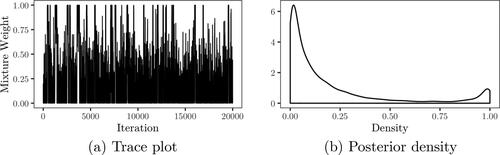
Figure 11. Trace plots of the kurtosis parameter, treatment coefficient and error and random effects variance based on Sampler 2.

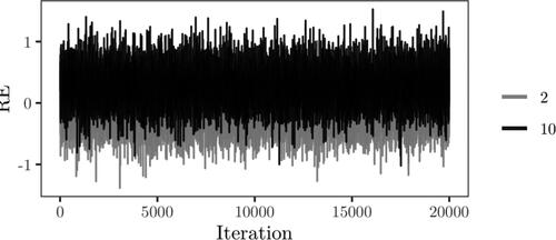
Figure 12. Posterior samples of random coefficients for individuals with id 1 and 20.

In Figure 13, the posterior density of the mixture weights are compared when fixing the kurtosis parameter to 0.6 and 1. The posterior median is estimated as 0.046 for the normal case, and 0.102 for $\kappa =0.6.$ The alternative hypothesis is thus strongly favored for both cases.

Figure 13. Posterior density of the mixture weights with the kurtosis parameter treated as a hyper-parameter.

We now consider testing whether the pretreatment levels of PAA are equal to the post-treatment levels, i.e., $H_0:{\mu }_1={\mu }_3$ vs. $H_1:{\mu }_1\ne {\mu }_3$ in (45). The test is carried out based on model (46) with null hypothesis ${\beta }_3=0.$ We only consider the comparison for $\kappa =0.6$ against κ = 1 for this case, with the comparison of the posterior densities of the mixture weights shown in Figure 14. The difference between the posterior densities is larger in comparison to Figure 13, with the posterior median for the normal case estimated as 0.90 and 0.772 for the kurtosis parameter set to 0.6. The difference in terms of posterior medians is thus large, although both cases tend to favor the null.

Figure 14. Posterior density of the mixture weights with the kurtosis parameter treated as a hyper-parameter.

For the frequentist model comparison, we consider tests based on Hotelling’s T² as in Example 4.2 in Crowder and Hand (1990). To test ${\mu }_1={\mu }_2={\mu }_3,$ the general null hypothesis $\mathit{H\mu }=\mathit{0}$ is considered, where $\mathit{\mu }=({\mu }_1,{\mu }_2,{\mu }_3)\prime$ and $$\mathit{H}=\left(\begin{array}{ccc}1& -1& 0\\ 1& 0& -1\end{array}\right).$$ When testing equality of pretreatment and post-treatment, H is set to the row vector $\mathit{H}=(10-1).$ For both cases, the test statistic is defined as (47) $$T^2=m{\overline{\mathit{y}}}^T{\mathit{H}}^T{(\mathit{HS}{\mathit{H}}^T)}^{-1}\mathit{H}\overline{\mathit{y}},$$(47) where $\overline{\mathit{y}}$ is the sample mean vector with elements ${\overline{y}}_j=n^{-1}{\sum }_{i=1}^m{y}_{ij}$ and S is the sample covariance matrix with elements $S_{jk}=(n-1){\sum }_{i=1}^m(y_{ij}-{\overline{y}}_j)(y_{ik}-{\overline{y}}_k).$ With the standard assumption of normality, $T^2\sim F_{q,n-q}$ under the null, where q is the number of rows of H and $F_{q,n-q}$ is the F distribution with q and n–q degrees of freedom. For the test of equality over all periods, $T^2=69.75$ which is $F_{2,10}$ distributed under the null with p-value virtually 0. For testing equality between pretreatment and post-treatment, $T^2=2.06$ which is $F_{1,11}$ distributed under the null with p-value 0.18. Thus, model choice based on Hotelling’s T² agrees with our results.

4. Conclusions

In this paper, the EPD class has been considered, in place of the standard normal assumption, in the context of Bayesian hypothesis testing of the fixed effects in LMMs for repeated measures. Tests have been carried out using a mixture representation rather than the traditional Bayes factor or posterior probability of a given hypothesis. In a simulation study, the kurtosis parameter is treated as a hyper-parameter to study its effect on model choice under increasing contamination by outliers. Main focus is on outliers in the error term, but outliers in the random effects are also considered. With no outliers in the random effects, results from the simulation study show that the EPD with a lower kurtosis than that of the normal distribution performs better in terms of consistently choosing the true model. A kurtosis of 0.6 is much less affected by increasing percentage of outliers and scaling factor, in comparison with the normal case. With increasing kurtosis, the sensitivity to outliers also increases. One notable result is that the difference between 0.6 and 0.7 is smaller than the difference between 0.9 and 1, both in terms of spread and average of the posterior median over the Monte Carlo replications. Increasing the outliers of the random effects had no effect on the result with the settings used in our simulation design.

When treating the kurtosis as a hyper-parameter in the applications to real data, we find in Example I that the normal case and $\kappa =0.6$ generally agree, albeit with the mixture parameter concentrating more around 1, i.e., favoring the null, for κ = 1. This was the case for both hyper-parameters considered for the variance of the fixed effects. Similarly, for Example II, we find that the results generally agree when treating the kurtosis parameter as a hyper-parameter for the test of all periods. When testing only pretreatment and post-treatment however, the difference was larger for the different values of the kurtosis parameter. One notable difference between Examples I and II is that the kurtosis parameter was sampled much closer to 1, i.e., normal, in Example I. When comparing the results in Example I to model choice in a frequentist setting with the usual normal assumption, we found that the full model under the alternative was favored. For Example II, we found that the model choice based on Hotelling’s T² agreed with our results.

The results from the applications and simulations indicate that using the general EPD class instead of a specific distribution as replacement, when the normality assumption is suspected, provides a flexible solution. For future research, the random effects could be included in the set of hypotheses in conjunction with extending to multiple hypotheses.

Acknowledgements

The authors are thankful to the editor, the associate editor and the two reviewers for their help and suggestions for the improvement of the article. Further, we gratefully acknowledge that the computations were enabled by resources provided by the Swedish National Infrastructure for Computing (SNIC) at UPPMAX partially funded by the Swedish Research Council through grant agreement no. 2018-05973.

Appendix: Gibbs sampler for repeated measures one-way-ANOVA

The posterior (24(24) $$p({\theta }_{\mu }|\mathit{y})\propto p(\mathit{y},\mathit{z}|\mathit{X},\mathit{Z},{\theta }_{\mu }\backslash \mathit{z})p(\mathit{\alpha }|\mathit{y},\mathit{X},\mathit{Z},{\theta }_{\mathit{\beta }})\prod _{i=1}^m{h}_{\kappa }(v_i)\pi (\mu |{\sigma }^2)\pi ({\sigma }^2)\pi (d)\pi (\kappa )\pi (\omega ).$$(24) ) is $$\begin{array}{c}p({\theta }_{\mu }|\mathit{y})\propto {({\sigma }^2)}^{-\frac{N}{2}}\hspace{0.17em}\text{exp}\hspace{0.17em}\left\{-\frac{1}{2{\sigma }^2}\sum _{i=1}^m{v}_i^{-2}{(y_i-z_{i1}\mu {\mathit{1}}_{n_i}-{\alpha }_i{\mathit{1}}_{n_i})}^T(y_i-z_{i1}\mu {\mathit{1}}_{n_i}-{\alpha }_i{\mathit{1}}_{n_i})\right\}\\ \times {\omega }^{{\sum }_{i=1}^n{z}_{i0}+a_2}{(1-\omega )}^{{\sum }_{i=1}^n{z}_{i1}}\left(\prod _{i=1}^m{(v_i^2)}^{-\frac{n_i}{2}}{h}_{\kappa }(v_i)\right){({\sigma }^2)}^{-\frac{m}{2}}\hspace{0.17em}\text{exp}\hspace{0.17em}\left\{-\frac{1}{2{\sigma }^{2}d}{\mathit{\alpha }}^T{\mathit{V}}^{-1}\mathit{\alpha }\right\}\\ \times {({\sigma }^2)}^{-\frac{1}{2}}\hspace{0.17em}\text{exp}\hspace{0.17em}\left\{-\frac{{({\mu }_0-\mu )}^2}{2{\sigma }^2{\sigma }_{\mu }^2}\right\}{({\sigma }^2)}^{-1-\frac{\nu }{2}}\hspace{0.17em}\text{exp}\hspace{0.17em}\left\{-\frac{\nu {\sigma }_0}{{\sigma }^2}\right\}{d}^{-1-\frac{\eta }{2}}{({\sigma }^2)}^{-\frac{\eta }{2}}\hspace{0.17em}\text{exp}\hspace{0.17em}\left\{-\frac{\eta {\tau }_0}{{\sigma }^{2}d}\right\}{1}_{[0,1]}(\kappa ).\end{array}$$ ${\sigma }^2,\mu$ and $\mathit{\alpha }$ are sampled jointly from $$({\sigma }^2,\mu ,\mathit{\alpha })\sim p({\sigma }^2|\mathit{y},{\theta }_{\mu }\backslash \{\mu ,\mathit{\alpha }\})p(\mu |\mathit{y},{\theta }_{\mu }\backslash \mathit{\alpha })p(\mathit{\alpha }|\mathit{y},{\theta }_{\mu }).$$ To derive the conditionals of σ and μ with $\mathit{\alpha }$ marginalized out, the likelihood is based on the marginal distribution of ${\mathit{y}}_i$ in (15(15) $$\left[\begin{array}{c}{\mathit{y}}_i\\ {\alpha }_i\end{array}\right]|v_i\sim {\mathcal{N}}_{n_i+1}\left(\left[\begin{array}{c}\mu {\mathit{1}}_{n_i}\\ 0\end{array}\right],{\sigma }^2{v}_i^2\left[\begin{array}{cc}\tilde{\mathbf{\Sigma }}& d{\mathit{1}}_{n_i}\\ d{\mathit{1}}_{n_i}^T& d\end{array}\right]\right),i=1,\dots ,m,$$(15) ) rather than the conditional. For ${\sigma }^2,$ $$\begin{array}{c}p({\sigma }^2,\mu |\mathit{y},{\theta }_{\mu }\backslash \{{\sigma }^2,\mathit{\alpha }\})\propto {\int }_{\mathit{\alpha }}p({\theta }_{\mu }|\mathit{y})d\mathit{\alpha }\propto \\ {({\sigma }^2)}^{-\frac{N}{2}}\hspace{0.17em}\text{exp}\hspace{0.17em}\left\{-\frac{1}{2{\sigma }^2}\sum _{i=1}^m{({\mathit{y}}_{\mathit{i}}-z_{i1}\mu {\mathit{1}}_{n_i})}^T{(v_i^2{\tilde{\mathbf{\Sigma }}}_i)}^{-1}({\mathit{y}}_{\mathit{i}}-z_{i1}\mu {\mathit{1}}_{n_i})\right\}\\ \times {({\sigma }^2)}^{-1-\frac{\nu }{2}}\hspace{0.17em}\text{exp}\hspace{0.17em}\left\{-\frac{\nu {\sigma }_0}{{\sigma }^2}\right\}{({\sigma }^2)}^{-\frac{\eta }{2}}\hspace{0.17em}\text{exp}\hspace{0.17em}\left\{-\frac{\eta {\tau }_0}{{\sigma }^{2}d}\right\}{({\sigma }^2)}^{-\frac{1}{2}}\hspace{0.17em}\text{exp}\hspace{0.17em}\left\{-\frac{{({\mu }_0-\mu )}^2}{2{\sigma }^2{\sigma }_{\mu }^2}\right\}.\end{array}$$ Next, μ is integrated out $$\begin{array}{c}p({\sigma }^2|\mathit{y},{\theta }_{\mu }\backslash \{{\sigma }^2,\mu ,\mathit{\alpha }\})\propto {({\sigma }^2)}^{-(1+\frac{1}{2}(N+\nu +\eta ))}\hspace{0.17em}\text{exp}\hspace{0.17em}\left\{-\frac{1}{2{\sigma }^2}(d^{-1}\eta {\tau }_0+\nu {\sigma }_0)\right\}\\ {\int }_{\mu }{({\sigma }^2)}^{-\frac{1}{2}}\hspace{0.17em}\text{exp}\hspace{0.17em}\left\{-\frac{1}{2{\sigma }^2}(\sum _{i=1}^m{({\mathit{y}}_{\mathit{i}}-z_{i1}\mu {\mathit{1}}_{n_i})}^T{(v_i^2{\tilde{\mathbf{\Sigma }}}_i)}^{-1}({\mathit{y}}_{\mathit{i}}-z_{i1}\mu {\mathit{1}}_{n_i})+\frac{{(\mu -{\mu }_0)}^2}{{\sigma }_0^2})\right\}d\mu \\ \propto {({\sigma }^2)}^{-(1+\frac{1}{2}(N+\nu +\eta ))}\hspace{0.17em}\text{exp}\hspace{0.17em}\left\{-\frac{1}{2{\sigma }^2}(d^{-1}\eta {\tau }_0+\nu {\sigma }_0)\right\}\hspace{0.17em}\text{exp}\hspace{0.17em}\{-\frac{1}{2{\sigma }^2}{[\sum _{i=1}^m({\mathit{y}}_i^T(v_i^2{\tilde{\mathbf{\Sigma }}}_i)}^{-1}{\mathit{y}}_i)+\\ \frac{{\mu }_0^2}{{\sigma }_{\mu }^2}-\tilde{\mu }(\sum _{i=1}^n{z}_{i1}{\mathit{1}}_{n_i}^T{(v_i^2{\tilde{\mathbf{\Sigma }}}_i)}^{-1}{\mathit{y}}_i+{\sigma }_{\mu }^{-2}{\mu }_0))]\}={({\sigma }^2)}^{-(1+\frac{1}{2}(N+\nu +\eta ))}\hspace{0.17em}\text{exp}\hspace{0.17em}\{-\frac{1}{2{\sigma }^2}[\\ (d^{-1}\eta {\tau }_0+\nu {\sigma }_0)+\sum _{i=1}^m{({\mathit{y}}_i-\tilde{\mu }{z}_{i1}{\mathit{1}}_{n_i})}^T{(v_i^2{\mathbf{\Sigma }}_i)}^{-1}({\mathit{y}}_i-\tilde{\mu }{z}_{i1}{\mathit{1}}_{n_i})+\frac{{({\mu }_0-\tilde{\mu })}^2}{{\sigma }_{\mu }^2}]\},\end{array}$$ where $$\tilde{\mu }={(\sum _{i=1}^m{z}_{i1}{\mathit{1}}_{n_i}^T{(v_i^2{\mathbf{\Sigma }}_i)}^{-1}{\mathit{1}}_{n_i}+{\mathbf{\Sigma }}_{\mu }^{-1})}^{-1}(\sum _{i=1}^m{z}_{i1}{\mathit{1}}_{n_i}^T{(v_i^2{\mathbf{\Sigma }}_i)}^{-1}{\mathit{y}}_i+{\mathbf{\Sigma }}_{\mu }^{-1}{\mu }_0).$$ The conditional distribution of ${\sigma }^2$ is then $${\sigma }^2|\mathit{y},{\theta }_{\mu }\backslash \{\mu ,\mathit{\alpha }\}\sim \frac{1}{{\chi }_{N+\eta +\nu }^2}(d^{-1}\eta {\tau }_0+\nu {\sigma }_0+\frac{{({\mu }_0-\tilde{\mu })}^2}{{\sigma }_{\mu }^2}+\sum _{i=1}^m{({\mathit{y}}_i-\tilde{\mu }{z}_{i1}{\mathit{1}}_{n_i})}^T{(v_i^2{\mathbf{\Sigma }}_i)}^{-1}({\mathit{y}}_i-\tilde{\mu }{z}_{i1}{\mathit{1}}_{n_i})).$$ The conditional distribution of μ with $\mathit{\alpha }$ marginalized is $$p(\mu |\mathit{y},{\theta }_{\mu }\backslash \{\mu ,\mathit{\alpha }\})\propto \hspace{0.17em}\text{exp}\hspace{0.17em}\{-\frac{1}{2{\sigma }^2}(\sum _{i=1}^m{({\mathit{y}}_i-z_{i1}\mu {\mathit{1}}_{n_i})}^T{(v_i^2{\tilde{\mathbf{\Sigma }}}_i)}^{-1}({\mathit{y}}_i-z_{i1}\mu {\mathit{1}}_{n_i})+\frac{{(\mu -{\mu }_0)}^2}{{\sigma }_{\mu }^2})\},$$ thus $$\mu |\mathit{y},{\theta }_{\mu }\backslash \{\mu ,\mathit{\alpha }\}\sim \mathcal{N}(\tilde{\mu },{\sigma }^2{(\sum _{i=1}^m{z}_{i1}{\mathit{1}}_{n_i}^T{(v_i^2{\tilde{\mathbf{\Sigma }}}_i)}^{-1}{\mathit{1}}_{n_i}+{\sigma }_{\mu }^{-2})}^{-1}).$$

References

- Arellano-Valle, R. B., H. Bolfarine, and V. H. Lachos. 2005. Skew-normal linear mixed models. Journal of Data Science 3:415–38.
- Bai, X., K. Chen, and W. Yao. 2016. Mixture of linear mixed models using multivariate t distribution. Journal of Statistical Computation and Simulation 86 (4):771–87. doi: 10.1080/00949655.2015.1036431.
- Bates, D., M. Mächler, B. Bolker, and S. Walker. 2015. Fitting linear mixed-effects models using lme4. Journal of Statistical Software 67 (1):1–48. doi: 10.18637/jss.v067.i01.
- Box, G. E. P., and G. C. Tiao. 1962. A further look at robustness via Bayes’s theorem. Biometrika 49 (3–4):419–32. doi: 10.2307/2333976.
- Box, G. E. P., and G. C. Tiao. 1964. A Bayesian approach to the importance of assumptions applied to the comparison of variances. Biometrika 51 (1–2):153–67. doi: 10.2307/2334203.
- Choy, S. T. B., and S. G. Walker. 2003. The extended exponential power distribution and Bayesian robustness. Statistics & Probability Letters 65 (3):227–32. doi: 10.1016/j.spl.2003.01.001.
- Crowder, M. J., and D. J. Hand. 1990. Analysis of repeated measures. Volume 41 of Monographs on statistics and applied probability. London: Chapman & Hall.
- Gómez, E., M. A. Gomez-Viilegas, and J. M. Marín. 1998. Multivariate generalization of the power exponential family of distributions. Communications in Statistics - Theory and Methods 27 (3):589–600. doi: 10.1080/03610929808832115.
- Gómez, E., M. A. Gómez-Villegas, and J. M. Marín. 2008. Multivariate exponential power distributions as mixtures of normal distributions with Bayesian applications. Communications in Statistics - Theory and Methods 37 (6):972–85. doi: 10.1080/03610920701762754.
- Haro-López, R. A., and A. F. M. Smith. 1999. On robust Bayesian analysis for location and scale parameters. Journal of Multivariate Analysis 70 (1):30–56. doi: 10.1006/jmva.1999.1820.
- Huggins, R. M. 1993. A robust approach to the analysis of repeated measures. Biometrics 49 (3):715–20. doi: 10.2307/2532192.
- Kamary, K. 2016. Non-informative priors and modelization via mixture models. PhD thesis., PSL Research University.
- Kass, R. E., and A. E. Raftery. 1995. Bayes factors. Journal of the American Statistical Association 90 (430):773–95. doi: 10.1080/01621459.1995.10476572.
- Lange, K. L., R. J. A. Little, and J. M. G. Taylor. 1989. Robust statistical modeling using the t distribution. Journal of the American Statistical Association 84 (408):881–96. doi: 10.2307/2290063.
- Lin, T. I., and J. C. Lee. 2008. Estimation and prediction in linear mixed models with skew-normal random effects for longitudinal data. Statistics in Medicine 27 (9):1490–507. doi: 10.1002/sim.3026.
- Lindsey, J. K. 1999. Multivariate elliptically contoured distributions for repeated measurements. Biometrics 55 (4):1277–80. doi: 10.1111/j.0006-341x.1999.01277.x.
- Mid-Michigan Medical Center. 1999. A study of oral condition of cancer patients. http://calcnet.mth.cmich.edu/org/spss/prj_cancer_data.htm.
- Nolan, J. P. 1997. Numerical calculation of stable densities and distribution functions. Communications in Statistics. Stochastic Models 13 (4):759–74. doi: 10.1080/15326349708807450.
- Park, T., and S. Min. 2016. Partially collapsed Gibbs sampling for linear mixed-effects models. Communications in Statistics - Simulation and Computation 45 (1):165–80. doi: 10.1080/03610918.2013.857687.
- Pinheiro, J. C., C. H. Liu, and Y. N. Wu. 2001. Efficient algorithm for robust estimation in linear mixed-effects models using a multivariate t-distribution. Journal of Computational and Graphical Statistics 10 (2):249–76. doi: 10.1198/10618600152628059.
- R Core Team. 2020. R: A language and environment for statistical computing. R Foundation for Statistical Computing, Vienna, Austria. https://www.R-project.org/.
- Rukhin, A. L., and A. Possolo. 2011. Laplace random effects models for interlaboratory studies. Computational Statistics & Data Analysis 55 (4):1815–27. doi: 10.1016/j.csda.2010.11.016.
- van Dyk, D. A., and T. Park. 2008. Partially collapsed Gibbs samplers: Theory and methods. Journal of the American Statistical Association 103 (482):790–6. doi: 10.1198/016214508000000409.
- Walker, S. G., and E. Gutierrex-Pena. 1998. Robustifying Bayesian procedures (with discussion). In Proceedings of the 6th Valencia International Meeting on Bayesian Statistics, Pages 685–713. Oxford University Press,
- Yavuz, F. G., and O. Arslan. 2018. Linear mixed model with Laplace distribution (LLMM). Statistical Papers 59 (1):271–89. doi: 10.1007/s00362-016-0763-x.
- Zhang, D., and M. Davidian. 2001. Linear mixed models with flexible distributions of random effects for longitudinal data. Biometrics 57 (3):795–802. doi: 10.1111/j.0006-341x.2001.00795.x.