A mixture autoregressive model based on Student’s t–distribution

Abstract

A new mixture autoregressive model based on Student’s t–distribution is proposed. A key feature of our model is that the conditional t–distributions of the component models are based on autoregressions that have multivariate t–distributions as their (low-dimensional) stationary distributions. That autoregressions with such stationary distributions exist is not immediate. Our formulation implies that the conditional mean of each component model is a linear function of past observations and the conditional variance is also time-varying. Compared to previous mixture autoregressive models our model may therefore be useful in applications where the data exhibits rather strong conditional heteroskedasticity. Our formulation also has the theoretical advantage that conditions for stationarity and ergodicity are always met and these properties are much more straightforward to establish than is common in nonlinear autoregressive models. An empirical example employing a realized kernel series constructed from S&P 500 high-frequency intraday data shows that the proposed model performs well in volatility forecasting. Our methodology is implemented in the freely available StMAR Toolbox for MATLAB.

Keywords:

• Conditional heteroskedasticity
• mixture model
• regime switching
• Student’s t–distribution

1. Introduction

Different types of mixture models are in widespread use in various fields. Overviews of mixture models can be found, for example, in the monographs of McLachlan and Peel (2000) and Frühwirth-Schnatter (2006). In this paper, we are concerned with mixture autoregressive models that were introduced by Le, Martin, and Raftery (1996) and further developed by Wong and Li (2000, 2001a, 2001b) (for further references, see Kalliovirta, Meitz, and Saikkonen (2015)).

In mixture autoregressive models the conditional distribution of the present observation given the past is a mixture distribution where the component distributions are obtained from linear autoregressive models. The specification of a mixture autoregressive model typically requires two choices: choosing a conditional distribution for the component models and choosing a functional form for the mixing weights. In a majority of existing models a Gaussian distribution is assumed whereas, in addition to constants, several different time-varying mixing weights (functions of past observations) have been considered in the literature.

Instead of a Gaussian distribution, Wong, Chan, and Kam (2009) proposed using Student’s t–distribution. A major motivation for this comes from the heavier tails of the t–distribution which allow the resulting model to better accommodate for the fat tails encountered in many observed time series, especially in economics and finance. In the model suggested by Wong, Chan, and Kam (2009), the conditional mean and conditional variance of each component model are the same as in the Gaussian case (a linear function of past observations and a constant, respectively), and what changes is the distribution of the independent and identically distributed error term: instead of a standard normal distribution, a Student’s t–distribution is used. This is a natural approach to formulate the component models and hence also a mixture autoregressive model based on the t–distribution.

In this paper, we also consider a mixture autoregressive model based on Student’s t–distribution, but our specification differs from that used by Wong, Chan, and Kam (2009). Our starting point is the characteristic feature of linear Gaussian autoregressions that stationary distributions (of consecutive observations) as well as conditional distributions are Gaussian. We imitate this feature by using a (multivariate) Student’s t–distribution and, as a first step, construct a linear autoregression in which both conditional and (low-dimensional) stationary distributions have Student’s t–distributions. This leads to a model where the conditional mean is as in the Gaussian case (a linear function of past observations) whereas the conditional variance is no longer constant but depends on a quadratic form of past observations. These linear models are then used as component models in our new mixture autoregressive model which we call the StMAR model.

Our StMAR model has some very attractive features. Like the model of Wong, Chan, and Kam (2009), it can be useful for modeling time series with leptokurtosis, regime switching, multimodality, persistence, and conditional heteroskedasticity. As the conditional variances of the component models are time-varying, the StMAR model can potentially accommodate for stronger forms of conditional heteroskedasticity than the model of Wong, Chan, and Kam (2009). Our formulation also has the theoretical advantage that, for a pth order model, the stationary distribution of p + 1 consecutive observations is fully known and is a mixture of particular Student’s t–distributions. Moreover, stationarity and ergodicity are simple consequences of the definition of the model and do not require complicated proofs.

Finally, a few notational conventions. All vectors are treated as column vectors and we write $\mathit{x}=(x_1,\dots ,x_n)$ for the vector x where the components x_i may be either scalars or vectors. The notation $\mathbf{X}\sim n_d(\mathit{\mu },\mathbf{\Gamma })$ signifies that the random vector X has a d–dimensional Gaussian distribution with mean $\mathit{\mu }$ and (positive definite) covariance matrix $\mathbf{\Gamma }.$ Similarly, by $\mathbf{X}\sim t_d(\mathit{\mu },\mathbf{\Gamma },\nu )$ we mean that X has a d–dimensional Student’s t–distribution with mean $\mathit{\mu }$, (positive definite) covariance matrix $\mathbf{\Gamma },$ and degrees of freedom ν (assumed to satisfy $\nu >2$); the density function and some properties of the multivariate Student’s t–distribution employed are given in Appendix A. The notation ${\mathbf{0}}_d$ (${\mathbf{1}}_d$) is used for a d–dimensional vector of zeros (ones), ${ı}_d$ signifies the vector $(1,0,\dots ,0)$ of dimension d, and the identity matrix of dimension d is denoted by I_d. The Kronecker product is denoted by ⊗, and vec(A) stacks the columns of matrix A on top of one another.

2. Linear Student’s t autoregressions

In order to formulate our new mixture model, this section briefly considers linear pth order autoregressions that have multivariate Student’s t–distributions as their stationary distributions. First, for motivation and to develop notation, consider a linear Gaussian autoregression z_t ($t=1,2,\dots$) generated by (1) $$z_t={\phi }_0+\sum _{i=1}^p{\phi }_i{z}_{t-i}+\sigma e_t,$$(1) where the error terms e_t are independent and identically distributed with a standard normal distribution, and the parameters satisfy ${\phi }_0\in \mathbb{R},\mathit{\phi }=({\phi }_1,\dots ,{\phi }_p)\in {\mathbb{S}}^p,$ and $\sigma >0,$ where (2) $${\mathbb{S}}^p=\{({\phi }_1,\dots ,{\phi }_p)\in {\mathbb{R}}^p:\phi \left(z\right)=1-\sum _{i=1}^p{\phi }_i{z}^i\ne 0\text{\hspace{0.5em}for\hspace{0.5em}}\left|\mathrm{z}\right|\le 1\}$$(2) is the stationarity region of a linear pth order autoregression. Denoting ${\mathit{z}}_t=(z_t,\dots ,z_{t-p+1})$ and ${\mathit{z}}_t^{+}=(z_t,{\mathit{z}}_{t-1}),$ it is well known that the stationary solution z_t to (1) satisfies (3) $$\begin{array}{c}{\mathit{z}}_t\sim n_p(\mu {\mathbf{1}}_p,{\mathbf{\Gamma }}_p),\\ {\mathit{z}}_t^{+}\sim n_{p+1}(\mu {\mathbf{1}}_{p+1},{\mathbf{\Gamma }}_{p+1}),\\ z_t|{\mathit{z}}_{t-1}\sim n_1({\phi }_0+\mathit{\phi }\prime {\mathit{z}}_{t-1},{\sigma }^2)=n_1(\mu +{\mathit{\gamma }}_p^{\prime }{\mathbf{\Gamma }}_p^{-1}({\mathit{z}}_{t-1}-\mu {\mathbf{1}}_p),{\sigma }^2),\end{array}$$(3) where the last relation defines the conditional distribution of z_t given ${\mathit{z}}_{t-1}$ and the quantities ${\mathbf{\Gamma }}_p,$ γ₀, ${\mathit{\gamma }}_p,$ μ, and ${\mathbf{\Gamma }}_{p+1}$ are defined via (4) $$\begin{array}{c}vec({\mathbf{\Gamma }}_p)={(I_{p^2}-(\Phi \otimes \Phi ))}^{-1}\hspace{0.17em}{ı}_{p^2}\hspace{0.17em}{\sigma }^2,\hspace{1em}\Phi =\left[\begin{array}{cc}{\phi }_1\cdots {\phi }_{p-1}& {\phi }_p\\ I_{p-1}& {\mathbf{0}}_{p-1}\end{array}\right],\\ {\gamma }_0={\sigma }^2+\mathit{\phi }\prime {\mathbf{\Gamma }}_p\mathit{\phi },\hspace{1em}{\mathit{\gamma }}_p={\mathbf{\Gamma }}_p\mathit{\phi },\hspace{1em}\mu ={\phi }_0/(1-{\phi }_1-\cdots -{\phi }_p),\hspace{1em}{\mathbf{\Gamma }}_{p+1}=\left[\begin{array}{cc}{\gamma }_0& {\mathit{\gamma }}_p^{\prime }\\ {\mathit{\gamma }}_p& {\mathbf{\Gamma }}_p\end{array}\right].\end{array}$$(4)

Two essential properties of linear Gaussian autoregressions are that they have the distributional features in (3)(3) $$\begin{array}{c}{\mathit{z}}_t\sim n_p(\mu {\mathbf{1}}_p,{\mathbf{\Gamma }}_p),\\ {\mathit{z}}_t^{+}\sim n_{p+1}(\mu {\mathbf{1}}_{p+1},{\mathbf{\Gamma }}_{p+1}),\\ z_t|{\mathit{z}}_{t-1}\sim n_1({\phi }_0+\mathit{\phi }\prime {\mathit{z}}_{t-1},{\sigma }^2)=n_1(\mu +{\mathit{\gamma }}_p^{\prime }{\mathbf{\Gamma }}_p^{-1}({\mathit{z}}_{t-1}-\mu {\mathbf{1}}_p),{\sigma }^2),\end{array}$$(3) and the representation in (1)(1) $$z_t={\phi }_0+\sum _{i=1}^p{\phi }_i{z}_{t-i}+\sigma e_t,$$(1) .

It is not immediately obvious that linear autoregressions based on Student’s t–distribution with similar properties exist (such models have, however, appeared at least in Spanos (1994), Heracleous and Spanos (2006), and Pitt and Walker (2006)). Suppose that for a random vector in ${\mathbb{R}}^{p+1}$ it holds that $(z,\mathit{z})\sim t_{p+1}(\mu {\mathbf{1}}_{p+1},{\mathbf{\Gamma }}_{p+1},\nu )$ where $\nu >2$ (and other notation is as above in (4)(4) $$\begin{array}{c}vec({\mathbf{\Gamma }}_p)={(I_{p^2}-(\Phi \otimes \Phi ))}^{-1}\hspace{0.17em}{ı}_{p^2}\hspace{0.17em}{\sigma }^2,\hspace{1em}\Phi =\left[\begin{array}{cc}{\phi }_1\cdots {\phi }_{p-1}& {\phi }_p\\ I_{p-1}& {\mathbf{0}}_{p-1}\end{array}\right],\\ {\gamma }_0={\sigma }^2+\mathit{\phi }\prime {\mathbf{\Gamma }}_p\mathit{\phi },\hspace{1em}{\mathit{\gamma }}_p={\mathbf{\Gamma }}_p\mathit{\phi },\hspace{1em}\mu ={\phi }_0/(1-{\phi }_1-\cdots -{\phi }_p),\hspace{1em}{\mathbf{\Gamma }}_{p+1}=\left[\begin{array}{cc}{\gamma }_0& {\mathit{\gamma }}_p^{\prime }\\ {\mathit{\gamma }}_p& {\mathbf{\Gamma }}_p\end{array}\right].\end{array}$$(4) ). Then (for details, see Appendix A) the conditional distribution of z given z is $z|\mathit{z}\sim t_1(\mu (\mathit{z}),{\sigma }^2(\mathit{z}),\nu +p),$ where (5) $$\mu (\mathit{z})={\phi }_0+\mathit{\phi }\prime \mathit{z},\mathrm{\hspace{1em}}\mathrm{\hspace{1em}}{\sigma }^2(\mathit{z})=\frac{\nu -2+{(\mathit{z}-\mu {\mathbf{1}}_p)}^{\prime }{\mathbf{\Gamma }}_p^{-1}(\mathit{z}-\mu {\mathbf{1}}_p)}{\nu -2+p}{\sigma }^2.$$(5)

We now state the following theorem (proofs of all theorems are in Appendix B).

Theorem 1.

Suppose ${\phi }_0\in \mathbb{R},\mathrm{\hspace{0.5em}}\mathit{\phi }=({\phi }_1,\dots ,{\phi }_p)\in {\mathbb{S}}^p,$ $\sigma >0$, and $\nu >2$. Then there exists a process ${\mathit{z}}_t=(z_t,\dots ,z_{t-p+1})$ ($t=0,1,2,\dots$) with the following properties.

1. The process ${\mathit{z}}_t$ ($t=1,2,\dots$) is a Markov chain on ${\mathbb{R}}^p$ with a stationary distribution characterized by the density function $t_p(\mu {\mathbf{1}}_p,{\mathbf{\Gamma }}_p,\nu )$. When ${\mathit{z}}_0\sim t_p(\mu {\mathbf{1}}_p,{\mathbf{\Gamma }}_p,\nu )$, we have, for $t=1,2,\dots$, that ${\mathit{z}}_t^{+}\sim t_{p+1}(\mu {\mathbf{1}}_{p+1},{\mathbf{\Gamma }}_{p+1},\nu )$ and the conditional distribution of z_t given ${\mathit{z}}_{t-1}$ is(6) $$z_t|{\mathit{z}}_{t-1}\sim t_1(\mu ({\mathit{z}}_{t-1}),{\sigma }^2({\mathit{z}}_{t-1}),\nu +p).$$(6)

2. Furthermore, for $t=1,2,\dots$, the process z_t has the representation(7) $$z_t={\phi }_0+\sum _{i=1}^p{\phi }_i z_{t-i}+{\sigma }_t\hspace{0.17em}{\epsilon }_t$$(7)

with conditional variance ${\sigma }_t^2={\sigma }^2({\mathit{z}}_{t-1})$ (see (5)), where the error terms ${\epsilon }_t$ form a sequence of independent and identically distributed random variables with a marginal $t_1(0,1,\nu +p)$ distribution and with ${\epsilon }_t$ independent of $\{z_s,s<t\}.$

Results (i) and (ii) in Theorem 1 are comparable to properties (3)(3) $$\begin{array}{c}{\mathit{z}}_t\sim n_p(\mu {\mathbf{1}}_p,{\mathbf{\Gamma }}_p),\\ {\mathit{z}}_t^{+}\sim n_{p+1}(\mu {\mathbf{1}}_{p+1},{\mathbf{\Gamma }}_{p+1}),\\ z_t|{\mathit{z}}_{t-1}\sim n_1({\phi }_0+\mathit{\phi }\prime {\mathit{z}}_{t-1},{\sigma }^2)=n_1(\mu +{\mathit{\gamma }}_p^{\prime }{\mathbf{\Gamma }}_p^{-1}({\mathit{z}}_{t-1}-\mu {\mathbf{1}}_p),{\sigma }^2),\end{array}$$(3) and (1)(1) $$z_t={\phi }_0+\sum _{i=1}^p{\phi }_i{z}_{t-i}+\sigma e_t,$$(1) in the Gaussian case. Part (i) shows that both the stationary and conditional distributions of z_t are t–distributions, whereas part (ii) clarifies the connection to standard AR(p) models. In contrast to linear Gaussian autoregressions, in this t–distributed case z_t is conditionally heteroskedastic and has an ‘AR(p)–ARCH(p)’ representation (here ARCH refers to autoregressive conditional heteroskedasticity).

3. A mixture autoregressive model based on Student’s t–distribution

3.1. Mixture autoregressive models

Let y_t ($t=1,2,\dots$) be the real-valued time series of interest, and let ${\mathcal{F}}_{t-1}$ denote the σ–algebra generated by $\{y_{t-j},\mathrm{ }j>0\}.$ We consider mixture autoregressive models for which the conditional density function of y_t given its past, $f(·|{\mathcal{F}}_{t-1}),$ is of the form (8) $$f(y_t|{\mathcal{F}}_{t-1})=\sum _{m=1}^M{\alpha }_{m,t}{f}_m(y_t|{\mathcal{F}}_{t-1}),$$(8) where the (positive) mixing weights ${\alpha }_{m,t}$ are ${\mathcal{F}}_{t-1}$–measurable and satisfy ${\sum }_{m=1}^M{\alpha }_{m,t}=1$ (for all t), and the $f_m(·|{\mathcal{F}}_{t-1}),m=1,\dots ,M,$ describe the conditional densities of M autoregressive component models. Different mixture models are obtained with different specifications of the mixing weights ${\alpha }_{m,t}$ and the conditional densities $f_m(·|{\mathcal{F}}_{t-1}).$

Starting with the specification of the conditional densities $f_m(·|{\mathcal{F}}_{t-1}),$ a common choice has been to assume the component models to be linear Gaussian autoregressions. For the mth component model ($m=1,\dots ,M$), denote the parameters of a pth order linear autoregression with ${\phi }_{m,0}\in \mathbb{R},\mathrm{\hspace{0.5em}}{\mathit{\phi }}_m=({\phi }_{m,1},\dots ,{\phi }_{m,p})\in {\mathbb{S}}^p,$ and ${\sigma }_m>0.$ Also set ${\mathit{y}}_{t-1}=(y_{t-1},\dots ,y_{t-p}).$ In the Gaussian case, the conditional densities in (8)(8) $$f(y_t|{\mathcal{F}}_{t-1})=\sum _{m=1}^M{\alpha }_{m,t}{f}_m(y_t|{\mathcal{F}}_{t-1}),$$(8) take the form ($m=1,\dots ,M$) $$f_m(y_t|{\mathcal{F}}_{t-1})=\frac{1}{{\sigma }_m}\varphi (\frac{y_t-{\mu }_{m,t}}{{\sigma }_m}),$$ where $\varphi (·)$ signifies the density function of a standard normal random variable, ${\mu }_{m,t}={\phi }_{m,0}+{\mathit{\phi }}_m^{\prime }{\mathit{y}}_{t-1}$ is the conditional mean function (of component m), and ${\sigma }_m^2>0$ is the conditional variance (of component m), often assumed to be constant. Instead of a Gaussian density, Wong, Chan, and Kam (2009) considered the case where $f_m(·|{\mathcal{F}}_{t-1})$ is the density of Student’s t–distribution with conditional mean and variance as above, ${\mu }_{m,t}={\phi }_{m,0}+{\mathit{\phi }}_m^{\prime }{\mathit{y}}_{t-1}$ and a constant ${\sigma }_m^2,$ respectively.

In this paper, we also consider a mixture autoregressive model based on Student’s t–distribution, but our formulation differs from that used by Wong, Chan, and Kam (2009). In Theorem 1 it was seen that linear autoregressions based on Student’s t–distribution naturally lead to the conditional distribution $t_1(\mu (·),{\sigma }^2(·),\nu +p)$ in (6)(6) $$z_t|{\mathit{z}}_{t-1}\sim t_1(\mu ({\mathit{z}}_{t-1}),{\sigma }^2({\mathit{z}}_{t-1}),\nu +p).$$(6) . Motivated by this, we consider a mixture autoregressive model in which the conditional densities $f_m(y_t|{\mathcal{F}}_{t-1})$ in (8)(8) $$f(y_t|{\mathcal{F}}_{t-1})=\sum _{m=1}^M{\alpha }_{m,t}{f}_m(y_t|{\mathcal{F}}_{t-1}),$$(8) are specified as (9) $$f_m(y_t|{\mathcal{F}}_{t-1})=t_1(y_t;{\mu }_{m,t},{\sigma }_{m,t}^2,{\nu }_m+p),$$(9) where the expressions for ${\mu }_{m,t}={\mu }_m({\mathit{y}}_{t-1})$ and ${\sigma }_{m,t}^2={\sigma }_m^2({\mathit{y}}_{t-1})$ are as in (5) except that z is replaced with ${\mathit{y}}_{t-1}$ and all the quantities therein are defined using the regime specific parameters ${\phi }_{m,0},{\mathit{\phi }}_m,$ σ_m, and ν_m (whenever appropriate a subscript m is added to previously defined notation, e.g., μ_m or ${\mathbf{\Gamma }}_{m,p}$). A key difference to the model of Wong, Chan, and Kam (2009) is that the conditional variance of component m is not constant but a function of ${\mathit{y}}_{t-1}.$ An explicit expression for the density in (9) can be obtained from Appendix A and is (10) $$f_m(y_t|{\mathcal{F}}_{t-1})=C({\nu }_m){\sigma }_{m,t}^{-1}{(1+{({\nu }_m+p-2)}^{-1}{(\frac{y_t-{\mu }_{m,t}}{{\sigma }_{m,t}})}^2)}^{-\frac{1+{\nu }_m+p}{2}},$$(10) where $C(\nu )=\frac{\Gamma ((1+\nu +p)/2)}{{(\pi (\nu +p-2))}^{1/2}\Gamma ((\nu +p)/2)}$ (and $\Gamma (·)$ signifies the gamma function).

Now consider the choice of the mixing weights ${\alpha }_{m,t}$ in (8)(8) $$f(y_t|{\mathcal{F}}_{t-1})=\sum _{m=1}^M{\alpha }_{m,t}{f}_m(y_t|{\mathcal{F}}_{t-1}),$$(8) . The most basic choice is to use constant mixing weights as in Wong and Li (2000) and Wong, Chan, and Kam (2009). Several different time-varying mixing weights have also been suggested, see, e.g., Wong and Li (2001a), Glasbey (2001), Lanne and Saikkonen (2003), Dueker, Sola, and Spagnolo (2007), and Kalliovirta, Meitz, and Saikkonen (2015, 2016).

In this paper, we propose mixing weights that are similar to those used by Glasbey (2001) and Kalliovirta, Meitz, and Saikkonen (2015). Specifically, we set (11) $${\alpha }_{m,t}=\frac{{\alpha }_m{t}_p({\mathit{y}}_{t-1};{\mu }_m{\mathbf{1}}_p,{\mathbf{\Gamma }}_{m,p},{\nu }_m)}{\sum _{n=1}^M{\alpha }_n{t}_p({\mathit{y}}_{t-1};{\mu }_n{\mathbf{1}}_p,{\mathbf{\Gamma }}_{n,p},{\nu }_n)},$$(11) where the ${\alpha }_m\in (0,1),\mathrm{\hspace{0.5em}}m=1,\dots ,M,$ are unknown parameters satisfying ${\sum }_{m=1}^M{\alpha }_m=1.$ Note that the Student’s t density appearing in (11)(11) $${\alpha }_{m,t}=\frac{{\alpha }_m{t}_p({\mathit{y}}_{t-1};{\mu }_m{\mathbf{1}}_p,{\mathbf{\Gamma }}_{m,p},{\nu }_m)}{\sum _{n=1}^M{\alpha }_n{t}_p({\mathit{y}}_{t-1};{\mu }_n{\mathbf{1}}_p,{\mathbf{\Gamma }}_{n,p},{\nu }_n)},$$(11) corresponds to the stationary distribution in Theorem 1(i): If the y_t’s were generated by a linear Student’s t autoregression described in Section 2 (with a subscript m added to all the notation therein), the stationary distribution of ${\mathit{y}}_{t-1}$ would be characterized by $t_p({\mathit{y}}_{t-1};{\mu }_m{\mathbf{1}}_p,{\mathbf{\Gamma }}_{m,p},{\nu }_m).$ Our definition of the mixing weights in (11)(11) $${\alpha }_{m,t}=\frac{{\alpha }_m{t}_p({\mathit{y}}_{t-1};{\mu }_m{\mathbf{1}}_p,{\mathbf{\Gamma }}_{m,p},{\nu }_m)}{\sum _{n=1}^M{\alpha }_n{t}_p({\mathit{y}}_{t-1};{\mu }_n{\mathbf{1}}_p,{\mathbf{\Gamma }}_{n,p},{\nu }_n)},$$(11) is different from that used in Glasbey (2001) and Kalliovirta, Meitz, and Saikkonen (2015) in that these authors employed the $n_p({\mathit{y}}_{t-1};{\mu }_m{\mathbf{1}}_p,{\mathbf{\Gamma }}_{m,p})$ density (corresponding to the stationary distribution of a linear Gaussian autoregression) instead of the Student’s t density $t_p({\mathit{y}}_{t-1};{\mu }_m{\mathbf{1}}_p,{\mathbf{\Gamma }}_{m,p},{\nu }_m)$ we use.

3.2. The Student’s t mixture autoregressive model

Equations (8)(8) $$f(y_t|{\mathcal{F}}_{t-1})=\sum _{m=1}^M{\alpha }_{m,t}{f}_m(y_t|{\mathcal{F}}_{t-1}),$$(8) , (9)(9) $$f_m(y_t|{\mathcal{F}}_{t-1})=t_1(y_t;{\mu }_{m,t},{\sigma }_{m,t}^2,{\nu }_m+p),$$(9) , and (11)(11) $${\alpha }_{m,t}=\frac{{\alpha }_m{t}_p({\mathit{y}}_{t-1};{\mu }_m{\mathbf{1}}_p,{\mathbf{\Gamma }}_{m,p},{\nu }_m)}{\sum _{n=1}^M{\alpha }_n{t}_p({\mathit{y}}_{t-1};{\mu }_n{\mathbf{1}}_p,{\mathbf{\Gamma }}_{n,p},{\nu }_n)},$$(11) define a model we call the Student’s t mixture autoregressive, or StMAR, model. When the autoregressive order p or the number of mixture components M need to be emphasized we refer to an StMAR(p,M) model. We collect the unknown parameters of an StMAR model in the vector $\mathit{\theta }=({\mathbf{\vartheta }}_1,\dots ,{\mathbf{\vartheta }}_M,{\alpha }_1,\dots ,{\alpha }_{M-1})$ ($(M(p+4)-1)\times 1$), where ${\mathbf{\vartheta }}_m=({\phi }_{m,0},{\mathit{\phi }}_m,{\sigma }_m^2,{\nu }_m)$ (with ${\mathbf{\phi }}_m\in {\mathbb{S}}^p,{\sigma }_m^2>0,$ and ${\nu }_m>2$) contains the parameters of each component model ($m=1,\dots ,M$) and the α_m’s are the parameters appearing in the mixing weights (11)(11) $${\alpha }_{m,t}=\frac{{\alpha }_m{t}_p({\mathit{y}}_{t-1};{\mu }_m{\mathbf{1}}_p,{\mathbf{\Gamma }}_{m,p},{\nu }_m)}{\sum _{n=1}^M{\alpha }_n{t}_p({\mathit{y}}_{t-1};{\mu }_n{\mathbf{1}}_p,{\mathbf{\Gamma }}_{n,p},{\nu }_n)},$$(11) ; the parameter α_M is not included due to the restriction ${\sum }_{m=1}^M{\alpha }_m=1.$

The StMAR model can also be presented in an alternative (but equivalent) form. To this end, let $P_{t-1}(·)$ signify the conditional probability of the indicated event given ${\mathcal{F}}_{t-1},$ and let ${\epsilon }_{m,t}$ be a sequence of independent and identically distributed random variables with a $t_1(0,1,{\nu }_m+p)$ distribution such that ${\epsilon }_{m,t}$ is independent of $\{y_{t-j},j>0\}$ ($m=1,\dots ,M$). Furthermore, let ${\mathit{s}}_t=(s_{1,t},\dots ,s_{M,t})$ be a sequence of (unobserved) M–dimensional random vectors such that, conditional on ${\mathcal{F}}_{t-1},\mathrm{\hspace{0.5em}}{\mathit{s}}_t$ and ${\epsilon }_{m,t}$ are independent (for all m). The components of ${\mathit{s}}_t$ are such that, for each t, exactly one of them takes the value one and others are equal to zero, with conditional probabilities $P_{t-1}(s_{m,t}=1)={\alpha }_{m,t},$ $m=1,\dots ,M.$ Now y_t can be expressed as (12) $$y_t=\sum _{m=1}^M{s}_{m,t}({\mu }_{m,t}+{\sigma }_{m,t}{\epsilon }_{m,t})=\sum _{m=1}^M{s}_{m,t}({\phi }_{m,0}+{\mathit{\phi }}_m^{\prime }{\mathit{y}}_{t-1}+{\sigma }_{m,t}{\epsilon }_{m,t}),$$(12) where ${\sigma }_{m,t}$ is as in (9). This formulation suggests that the mixing weights ${\alpha }_{m,t}$ can be thought of as (conditional) probabilities that determine which one of the M autoregressive components of the mixture generates the observation y_t.

It turns out that the StMAR model has some very attractive theoretical properties; the carefully chosen conditional densities in (9)(9) $$f_m(y_t|{\mathcal{F}}_{t-1})=t_1(y_t;{\mu }_{m,t},{\sigma }_{m,t}^2,{\nu }_m+p),$$(9) and the mixing weights in (11)(11) $${\alpha }_{m,t}=\frac{{\alpha }_m{t}_p({\mathit{y}}_{t-1};{\mu }_m{\mathbf{1}}_p,{\mathbf{\Gamma }}_{m,p},{\nu }_m)}{\sum _{n=1}^M{\alpha }_n{t}_p({\mathit{y}}_{t-1};{\mu }_n{\mathbf{1}}_p,{\mathbf{\Gamma }}_{n,p},{\nu }_n)},$$(11) are crucial in obtaining these properties. The following theorem shows that there exists a choice of initial values ${\mathit{y}}_0$ such that ${\mathit{y}}_t$ is a stationary and ergodic Markov chain. Importantly, an explicit expression for the stationary distribution is also provided.

Theorem 2.

Consider the StMAR process y_t generated by (8)(8) $$f(y_t|{\mathcal{F}}_{t-1})=\sum _{m=1}^M{\alpha }_{m,t}{f}_m(y_t|{\mathcal{F}}_{t-1}),$$(8) , (9)(9) $$f_m(y_t|{\mathcal{F}}_{t-1})=t_1(y_t;{\mu }_{m,t},{\sigma }_{m,t}^2,{\nu }_m+p),$$(9) , and (11)(11) $${\alpha }_{m,t}=\frac{{\alpha }_m{t}_p({\mathit{y}}_{t-1};{\mu }_m{\mathbf{1}}_p,{\mathbf{\Gamma }}_{m,p},{\nu }_m)}{\sum _{n=1}^M{\alpha }_n{t}_p({\mathit{y}}_{t-1};{\mu }_n{\mathbf{1}}_p,{\mathbf{\Gamma }}_{n,p},{\nu }_n)},$$(11) (or (12)(12) $$y_t=\sum _{m=1}^M{s}_{m,t}({\mu }_{m,t}+{\sigma }_{m,t}{\epsilon }_{m,t})=\sum _{m=1}^M{s}_{m,t}({\phi }_{m,0}+{\mathit{\phi }}_m^{\prime }{\mathit{y}}_{t-1}+{\sigma }_{m,t}{\epsilon }_{m,t}),$$(12) and (11)(11) $${\alpha }_{m,t}=\frac{{\alpha }_m{t}_p({\mathit{y}}_{t-1};{\mu }_m{\mathbf{1}}_p,{\mathbf{\Gamma }}_{m,p},{\nu }_m)}{\sum _{n=1}^M{\alpha }_n{t}_p({\mathit{y}}_{t-1};{\mu }_n{\mathbf{1}}_p,{\mathbf{\Gamma }}_{n,p},{\nu }_n)},$$(11) ) with the conditions φ_m$\in {\mathbb{S}}^p$ and ${\nu }_m>2$ satisfied for all $m=1,\dots ,M$. Then ${\mathit{y}}_t=(y_t,\dots ,y_{t-p+1})$ ($t=1,2,\dots$) is a Markov chain on ${\mathbb{R}}^p$ with a stationary distribution characterized by the density $f(\mathit{y};\mathit{\theta })={\sum }_{m=1}^M{\alpha }_m{t}_p(\mathit{y};{\mu }_m{\mathbf{1}}_p,{\mathbf{\Gamma }}_{m,p},{\nu }_m)$. Moreover, ${\mathit{y}}_t$ is ergodic.

As can be seen from the proof of Theorem 2 (in Appendix B), the Markov property, stationarity, and ergodicity are obtained as reasonably simple consequences of the definition of the StMAR model. The stationary distribution of ${\mathit{y}}_t$ is a mixture of M p–dimensional t–distributions with constant mixing weights α_m. Hence, moments of the stationary distribution of order smaller than $\min ({\nu }_1,\dots ,{\nu }_M)$ exist and are finite. Furthermore, the stationary distribution of the vector $(y_t,{\mathit{y}}_{t-1})$ is also a mixture of M t–distributions with density of the same form, ${\sum }_{m=1}^M{\alpha }_m{t}_{p+1}({\mu }_m{\mathbf{1}}_{p+1},{\mathbf{\Gamma }}_{m,p+1},{\nu }_m)$ (for details, see Appendix B). Thus the mean, variance, and first p autocovariances of y_t are (here the connection between ${\gamma }_{m,j}$ and ${\mathbf{\Gamma }}_{m,p+1}$ is as in (4)(4) $$\begin{array}{c}vec({\mathbf{\Gamma }}_p)={(I_{p^2}-(\Phi \otimes \Phi ))}^{-1}\hspace{0.17em}{ı}_{p^2}\hspace{0.17em}{\sigma }^2,\hspace{1em}\Phi =\left[\begin{array}{cc}{\phi }_1\cdots {\phi }_{p-1}& {\phi }_p\\ I_{p-1}& {\mathbf{0}}_{p-1}\end{array}\right],\\ {\gamma }_0={\sigma }^2+\mathit{\phi }\prime {\mathbf{\Gamma }}_p\mathit{\phi },\hspace{1em}{\mathit{\gamma }}_p={\mathbf{\Gamma }}_p\mathit{\phi },\hspace{1em}\mu ={\phi }_0/(1-{\phi }_1-\cdots -{\phi }_p),\hspace{1em}{\mathbf{\Gamma }}_{p+1}=\left[\begin{array}{cc}{\gamma }_0& {\mathit{\gamma }}_p^{\prime }\\ {\mathit{\gamma }}_p& {\mathbf{\Gamma }}_p\end{array}\right].\end{array}$$(4) ) $$\mu \stackrel{\mathit{def}}{=}E\left[y_t\right]=\sum _{m=1}^M{\alpha }_m{\mu }_m,\hspace{1em}{\gamma }_j\stackrel{\mathit{def}}{=}Cov[y_t,y_{t-j}]=\sum _{m=1}^M{\alpha }_m{\gamma }_{m,j}+\sum _{m=1}^M{\alpha }_m{({\mu }_m-\mu )}^2,\mathrm{\hspace{0.5em}}j=0,\dots ,p.$$

Subvectors of $(y_t,{\mathit{y}}_{t-1})$ also have stationary distributions that belong to the same family (but this does not hold for higher dimensional vectors such as $(y_{t+1},y_t,{\mathit{y}}_{t-1})$).

The fact that an explicit expression for the stationary (marginal) distribution of the StMAR model is available is not only convenient but also quite exceptional among mixture autoregressive models or other related nonlinear autoregressive models (such as threshold or smooth transition models). Previously, similar results have been obtained by Glasbey (2001) and Kalliovirta, Meitz, and Saikkonen (2015) in the context of mixture autoregressive models that are of the same form but based on the Gaussian distribution (for a few rather simple first order examples involving other models, see Tong (2011, Section 4.2)).

From the definition of the model, the conditional mean and variance of y_t are obtained as (13) $$E[y_t|{\mathcal{F}}_{t-1}]=\sum _{m=1}^M{\alpha }_{m,t}{\mu }_{m,t},\hspace{1em}\mathit{Var}[y_t|{\mathcal{F}}_{t-1}]=\sum _{m=1}^M{\alpha }_{m,t}{\sigma }_{m,t}^2+\sum _{m=1}^M{\alpha }_{m,t}{({\mu }_{m,t}-\sum _{n=1}^M{\alpha }_{n,t}{\mu }_{n,t})}^2.$$(13)

Except for the different definition of the mixing weights, the conditional mean is as in the Gaussian mixture autoregressive model of Kalliovirta, Meitz, and Saikkonen (2015). This is due to the well-known fact that in the multivariate t–distribution the conditional mean is of the same linear form as in the multivariate Gaussian distribution. However, unlike in the Gaussian case, the conditional variance of the multivariate t–distribution is not constant. Therefore, in (13)(13) $$E[y_t|{\mathcal{F}}_{t-1}]=\sum _{m=1}^M{\alpha }_{m,t}{\mu }_{m,t},\hspace{1em}\mathit{Var}[y_t|{\mathcal{F}}_{t-1}]=\sum _{m=1}^M{\alpha }_{m,t}{\sigma }_{m,t}^2+\sum _{m=1}^M{\alpha }_{m,t}{({\mu }_{m,t}-\sum _{n=1}^M{\alpha }_{n,t}{\mu }_{n,t})}^2.$$(13) we have the time-varying variance component ${\sigma }_{m,t}^2$ which in the models of Kalliovirta, Meitz, and Saikkonen (2015) and Wong, Chan, and Kam (2009) is constant (in the latter model the mixing weights are also constants). In (13)(13) $$E[y_t|{\mathcal{F}}_{t-1}]=\sum _{m=1}^M{\alpha }_{m,t}{\mu }_{m,t},\hspace{1em}\mathit{Var}[y_t|{\mathcal{F}}_{t-1}]=\sum _{m=1}^M{\alpha }_{m,t}{\sigma }_{m,t}^2+\sum _{m=1}^M{\alpha }_{m,t}{({\mu }_{m,t}-\sum _{n=1}^M{\alpha }_{n,t}{\mu }_{n,t})}^2.$$(13) both the mixing weights ${\alpha }_{m,t}$ and the variance components ${\sigma }_{m,t}^2$ are functions of ${\mathit{y}}_{t-1},$ implying that the conditional variance exhibits nonlinear autoregressive conditional heteroskedasticity. Compared to the aforementioned previous models our model may therefore be useful in applications where the data exhibits rather strong conditional heteroskedasticity.

In many applications in economics, finance, and other fields, the data is often multimodal and contains periods with markedly different behaviors. In such a situation a multiple regime StMAR model would be more appropriate than a linear model. This applies also to the StMAR model with a single regime (M = 1) which corresponds to the linear Student’s t autoregression considered in Section 2. Furthermore, the conditional mean and variance are much more flexible in a mixture model than in a linear one.

4. Estimation

The parameters of an StMAR model can be estimated by the method of maximum likelihood (details of the numerical optimization methods employed and of simulation experiments are available in the Supplementary Appendix). As the stationary distribution of the StMAR process is known it is even possible to make use of initial values and construct the exact likelihood function and obtain exact maximum likelihood estimates. Assuming the observed data $y_{-p+1},\dots ,y_0,y_1,\dots ,y_T$ and stationary initial values, the log-likelihood function takes the form (14) $$L_T(\mathit{\theta })=\hspace{0.17em}\text{log}\hspace{0.17em}(\sum _{m=1}^M{\alpha }_m{t}_p({\mathit{y}}_0;{\mu }_m{\mathbf{1}}_p,{\mathbf{\Gamma }}_{m,p},{\nu }_m))+\sum _{t=1}^T{l}_t(\mathit{\theta }),$$(14) where (15) $$l_t(\mathit{\theta })=\hspace{0.17em}\text{log}\hspace{0.17em}(\sum _{m=1}^M{\alpha }_{m,t}{t}_1(y_t;{\mu }_{m,t},{\sigma }_{m,t}^2,{\nu }_m+p)).$$(15)

An explicit expression for the density appearing in (15)(15) $$l_t(\mathit{\theta })=\hspace{0.17em}\text{log}\hspace{0.17em}(\sum _{m=1}^M{\alpha }_{m,t}{t}_1(y_t;{\mu }_{m,t},{\sigma }_{m,t}^2,{\nu }_m+p)).$$(15) is given in (10)(10) $$f_m(y_t|{\mathcal{F}}_{t-1})=C({\nu }_m){\sigma }_{m,t}^{-1}{(1+{({\nu }_m+p-2)}^{-1}{(\frac{y_t-{\mu }_{m,t}}{{\sigma }_{m,t}})}^2)}^{-\frac{1+{\nu }_m+p}{2}},$$(10) , and the notation for ${\mu }_{m,t}$ and ${\sigma }_{m,t}^2$ is explained after (9)(9) $$f_m(y_t|{\mathcal{F}}_{t-1})=t_1(y_t;{\mu }_{m,t},{\sigma }_{m,t}^2,{\nu }_m+p),$$(9) . Although not made explicit, ${\alpha }_{m,t},{\mu }_{m,t},$ and ${\sigma }_{m,t}^2,$ as well as the quantities μ_m, ${\mathit{\gamma }}_{m,p},$ and ${\Gamma }_{m,p},$ depend on the parameter vector $\mathit{\theta }.$

In (14)(14) $$L_T(\mathit{\theta })=\hspace{0.17em}\text{log}\hspace{0.17em}(\sum _{m=1}^M{\alpha }_m{t}_p({\mathit{y}}_0;{\mu }_m{\mathbf{1}}_p,{\mathbf{\Gamma }}_{m,p},{\nu }_m))+\sum _{t=1}^T{l}_t(\mathit{\theta }),$$(14) it has been assumed that the initial values ${\mathit{y}}_0$ are generated by the stationary distribution. If this assumption seems inappropriate one can condition on initial values and drop the first term on the right hand side of (14)(14) $$L_T(\mathit{\theta })=\hspace{0.17em}\text{log}\hspace{0.17em}(\sum _{m=1}^M{\alpha }_m{t}_p({\mathit{y}}_0;{\mu }_m{\mathbf{1}}_p,{\mathbf{\Gamma }}_{m,p},{\nu }_m))+\sum _{t=1}^T{l}_t(\mathit{\theta }),$$(14) . In what follows we assume that estimation is based on this conditional log-likelihood, namely $L_T^{(c)}(\mathit{\theta })=T^{-1}{\sum }_{t=1}^T{l}_t(\mathit{\theta })$ which we, for convenience, have also scaled with the sample size. Maximizing $L_T^{(c)}(\mathit{\theta })$ with respect to $\mathit{\theta }$ yields the maximum likelihood estimator denoted by ${\widehat{\mathit{\theta }}}_T.$

The permissible parameter space of $\mathit{\theta },$ denoted by $\Theta ,$ needs to be constrained in various ways. The stationarity conditions ${\mathit{\phi }}_m\in {\mathbb{S}}^p,$ the positivity of the variances ${\sigma }_m^2,$ and the conditions ${\nu }_m>2$ ensuring existence of second moments are all assumed to hold (for $m=1,\dots ,M$). Throughout we assume that the number of mixture components M is known, and this also entails the requirement that the parameters α_m ($m=1,\dots ,M$) are strictly positive (and strictly less than unity whenever M > 1). Further restrictions are required to ensure identification. Denoting the true parameter value by ${\mathit{\theta }}_0$ and assuming stationary initial values, the condition needed is that $l_t(\mathit{\theta })=l_t({\mathit{\theta }}_0)$ almost surely only if $\mathit{\theta }={\mathit{\theta }}_0.$ An additional assumption needed for this is (16) $${\alpha }_1>\cdots >{\alpha }_M>0\text{\hspace{0.5em}and\hspace{0.5em}}{\mathbf{\vartheta }}_i={\mathbf{\vartheta }}_j \text{only} \text{if} 1\le i=j\le M.$$(16)

From a practical point of view this assumption is not restrictive because what it essentially requires is that the M component models cannot be ‘relabeled’ and the same StMAR model obtained. We summarize the restrictions imposed on the parameter space as follows.

Assumption 1.

The true parameter value ${\mathit{\theta }}_0$ is an interior point of $\Theta$, where $\Theta$ is a compact subset of $\{\mathit{\theta }=({\mathbf{\vartheta }}_1,\dots ,{\mathbf{\vartheta }}_M,{\alpha }_1,\dots ,{\alpha }_{M-1})\in {\mathbb{R}}^{M(p+3)}\times {(0,1)}^{M-1}:{\mathit{\phi }}_m\in {\mathbb{S}}^p, {\sigma }_m^2>0,\mathit{\text{and}}\mathrm{ }{\nu }_m>2 \mathit{for}\mathrm{\hspace{0.5em}}\mathit{all}\mathrm{ }m=1,\dots ,M, \mathit{and}\mathrm{\hspace{0.5em}}(16)\mathrm{\hspace{0.5em}}\mathit{holds}\}.$

Asymptotic properties of the maximum likelihood estimator can now be established under conventional high-level conditions. Denote $\mathcal{I}(\mathit{\theta })=E[\frac{\partial l_t(\mathit{\theta })}{\partial \mathit{\theta }}\frac{\partial l_t(\mathit{\theta })}{\partial \mathit{\theta }\prime }]$ and $\mathcal{J}(\mathit{\theta })=E[\frac{{\partial }^2{l}_t(\mathit{\theta })}{\partial \mathit{\theta }\partial \mathit{\theta }\prime }].$

Theorem 3.

Suppose y_t is generated by the stationary and ergodic StMAR process of Theorem 2 and that Assumption 1 holds. Then ${\widehat{\mathit{\theta }}}_T$ is strongly consistent, i.e., ${\widehat{\mathit{\theta }}}_T\to {\mathit{\theta }}_0$ almost surely. Suppose further that (i) $T^{1/2}\frac{\partial }{\partial \mathit{\theta }}{L}_T^{(c)}({\mathit{\theta }}_0)\stackrel{d}{\to }N(0,\mathcal{I}({\mathit{\theta }}_0))$ with $\mathcal{I}({\mathit{\theta }}_0)$ finite and positive definite, (ii) $\mathcal{J}({\mathit{\theta }}_0)=-\mathcal{I}({\mathit{\theta }}_0)$, and (iii) $E[\underset{\mathit{\theta }\in {\Theta }_0}{\sup }|\frac{{\partial }^2{l}_t(\mathit{\theta })}{\partial \mathit{\theta }\partial \mathit{\theta }\prime }|]<\infty$ for some ${\Theta }_0$, a compact convex set contained in the interior of $\Theta$ that has ${\mathit{\theta }}_0$ as an interior point. Then $T^{1/2}({\widehat{\mathit{\theta }}}_T-{\mathit{\theta }}_0)\stackrel{d}{\to }N(0,-\mathcal{J}{({\mathit{\theta }}_0)}^{-1}).$

Of the conditions in this theorem, (i) states that a central limit theorem holds for the score vector (evaluated at ${\mathit{\theta }}_0$) and that the information matrix is positive definite, (ii) is the information matrix equality, and (iii) ensures the uniform convergence of the Hessian matrix (in some neighborhood of ${\mathit{\theta }}_0$). These conditions are standard but their verification may be tedious.

Theorem 3  shows that the conventional limiting distribution applies to the maximum likelihood estimator ${\widehat{\mathit{\theta }}}_T,$ which implies the applicability of standard likelihood-based tests. It is worth noting, however, that here a correct specification of the number of autoregressive components M is required. In particular, if the number of component models is chosen too large then some parameters of the model are not identified and, consequently, the result of Theorem 3 and the validity of the related tests break down. This particularly happens when one tests for the number of component models. Such tests for mixture autoregressive models with Gaussian conditional densities (see (8)(8) $$f(y_t|{\mathcal{F}}_{t-1})=\sum _{m=1}^M{\alpha }_{m,t}{f}_m(y_t|{\mathcal{F}}_{t-1}),$$(8) ) are developed by Meitz and Saikkonen (2021). The testing problem is highly nonstandard and extending their results to the present case is beyond the scope of this paper.

Instead of formal tests, in our empirical application we take a pragmatic approach and resort to the use of information criteria to infer which model fits the data best. Similar approaches have also been used by Wong, Chan, and Kam (2009) and others. Note that once the number of regimes is (correctly) chosen, standard likelihood-based inference can be used to choose regime-wise autoregressive orders and to test other hypotheses of interest. Validity of (quantile) residual-based misspecification tests to check for model adequacy also relies on the correct specification of the number of regimes.

5. Empirical example

Modeling and forecasting financial market volatility is key to manage risk. In this application we use the realized kernel of Barndorff-Nielsen et al. (2008) as a proxy for latent volatility. We obtained daily realized kernel data over the period 3 January 2000 through 20 May 2016 for the S&P 500 index from the Oxford-Man Institute’s Realized Library v0.2 (Heber et al. 2009). Figure 1 shows the in-sample period (Jan 3, 2000–June 3, 2014; 3597 observations) for the S&P 500 realized kernel data (${\text{RK}}_t$), which is nonnegative with a distribution exhibiting substantial skewness and excess kurtosis (sample skewness 14.3, sample kurtosis 380.8). We follow the related literature which frequently use logarithmic realized kernel ($\text{log}\hspace{0.17em}({\text{RK}}_t)$), to avoid imposing additional parameter constraints, and to obtain a more symmetric distribution, often taken to be approximately Gaussian. The $\text{log}\hspace{0.17em}({\text{RK}}_t)$ data, also shown in Figure 1, has a sample skewness of 0.5 and kurtosis of 3.5. Visual inspection of the time series plots of the ${\text{RK}}_t$ and $\text{log}\hspace{0.17em}({\text{RK}}_t)$ data suggests that the two series exhibit changes at least in levels and potentially also in variability. A kernel estimate of the density function of the $\text{log}\hspace{0.17em}({\text{RK}}_t)$ series also suggest the potential presence of multiple regimes.

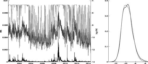
Figure 1. Left panel: Daily ${\text{RK}}_t$ (lower solid) and $\text{log}\hspace{0.17em}({\text{RK}}_t)$ (upper solid), and mixing weights based on the estimates of the StMAR(4,2) model in Table 1 (dot-dash) for the $\text{log}\hspace{0.17em}({\text{RK}}_t)$ series. The mixing weights ${\widehat{\alpha }}_{1,t}$ are scaled from $(0, 1)$ to $(\min \hspace{0.17em}\text{log}\hspace{0.17em}({\text{RK}}_t), \max \hspace{0.17em}\text{log}\hspace{0.17em}({\text{RK}}_t)).$ Right panel: A kernel density estimate of the $\text{log}\hspace{0.17em}({\text{RK}}_t)$ observations (solid), and the mixture density (dashes) implied by the same StMAR model as in the left panel.

For brevity, we focus our attention on StMAR models with $p=1,2,3,4$ and M = 1, 2, 3; higher-order models were also tried but their forecasting performance was qualitatively similar to the models with $p\le 4.$ Following Wong and Li (2001a), Wong, Chan, and Kam (2009), and Li et al. (2015), we use information criteria for model comparison. Of these models, the Akaike information criterion (aic) and the Hannan-Quinn information criterion (hqc) favor the StMAR(4,3) model, and the Bayesian information criterion (bic) the simpler StMAR(4,1) model. Estimation results for these two models, as well as the intermediate StMAR(4,2) model, are reported in Table 1. As the estimated mixture weight of the third component of the StMAR(4,3) model is rather small (${\widehat{\alpha }}_3\approx 0.023$) and the first two components are very similar to the StMAR(4,2) model, including this intermediate StMAR(4,2) model seems reasonable. In view of the approximate standard errors in Table 1, the estimation accuracy appears quite reasonable except for the degrees of freedom parameters (for large values of the degrees of freedom parameters the likelihood function becomes very flat; in particular ${\widehat{\nu }}_3$ and its standard error may be rather inaccurate). Taking the sum of the autoregressive parameters as a measure of persistence, we find that the estimated persistence for the first regime of the StMAR(4,2) is 0.909 and 0.489 for the second regime, suggesting that persistence is rather strong in the first regime and moderate in the second regime.

Table 1. Parameter estimates for three selected StMAR models and the $\text{log}\hspace{0.17em}({\text{RK}}_t)$ data over the period 3 January 2000–3 June 2014.

	StMAR(4, 1)		StMAR(4, 2)		StMAR(4, 3)
${\phi }_{1,0}$	–0.746	(0.089)	–0.851	(0.112)	–0.859	(0.116)
${\phi }_{1,1}$	0.428	(0.017)	0.432	(0.024)	0.407	(0.024)
${\phi }_{1,2}$	0.224	(0.019)	0.221	(0.025)	0.216	(0.025)
${\phi }_{1,3}$	0.121	(0.019)	0.122	(0.025)	0.123	(0.025)
${\phi }_{1,4}$	0.150	(0.017)	0.134	(0.024)	0.162	(0.024)
${\sigma }_1^2$	0.298	(0.011)	0.285	(0.015)	0.283	(0.015)
ν1	11.999	(1.173)	10.510	(1.628)	10.695	(2.070)
${\phi }_{2,0}$			–5.381	(1.036)	–5.745	(1.050)
${\phi }_{2,1}$			0.289	(0.046)	0.300	(0.049)
${\phi }_{2,2}$			0.129	(0.049)	0.121	(0.051)
${\phi }_{2,3}$			0.023	(0.047)	0.015	(0.049)
${\phi }_{2,4}$			0.047	(0.053)	0.019	(0.056)
${\sigma }_2^2$			0.287	(0.022)	0.290	(0.023)
ν2			29.031	(1.957)	32.143	(4.503)
${\phi }_{3,0}$					–5.459	(1.068)
${\phi }_{3,1}$					0.479	(0.102)
${\phi }_{3,2}$					0.334	(0.125)
${\phi }_{3,3}$					0.206	(0.111)
${\phi }_{3,4}$					–0.728	(0.122)
${\sigma }_3^2$					0.088	(0.032)
ν3					35438.182	(0.137)
α1			0.724	(0.065)	0.721	(0.060)
α2					0.256	(0.062)
$T{L}_T^{(c)}({\widehat{\mathit{\theta }}}_T)$	–2854.153		–2832.665		–2814.469
aic	5722.306		5695.330		5674.937
hqc	5737.741		5728.406		5725.653
bic	5765.613		5788.131		5817.233

Numbers in parentheses are standard errors based on a numerical Hessian.

Numerous alternative models for volatility proxies have been proposed. We employ Corsi’s (2009) heterogeneous autoregressive (HAR) model as it is arguably the most popular reference model for forecasting proxies such as the realized kernel. We also consider a pth-order autoregression as the AR(p) often performs well in volatility proxy forecasting. The StMAR models are estimated using maximum likelihood, and the reference AR and HAR models by ordinary least squares. We use a fixed scheme, where the parameters of our volatility models are estimated just once using data from Jan 3, 2000–June 3, 2014. These estimates are then used to generate all forecasts. The remaining 496 observations of our sample are used to compare the forecasts from the alternative models. As discussed in Kalliovirta, Meitz, and Saikkonen (2016), computing multi-step-ahead forecasts for mixture models like the StMAR is rather complicated. For this reason we use computer driven forecasts to predict future volatility: For each out-of-sample date T, and for each alternative model, we simulate 1,000,000 sample paths. Each path is of length 22 (representing one trading month) and conditional on the information available at date T. In these simulations unknown parameters are replaced by their estimates. As the simulated paths are for $\text{log}\hspace{0.17em}({\text{RK}}_t),$ and our object of interest is ${\text{RK}}_t,$ an exponential transformation is applied.

We examine daily, weekly (5 day), biweekly (10 day), and monthly (22 day) volatility forecasts generated by the alternative models; for instance, the weekly volatility forecast at date T is the forecast for ${\text{RK}}_{T+1}+\cdots +{\text{RK}}_{T+5}$ (the 5-day-ahead cumulative realized kernel). Table 2 reports the percentage shares of (1, 5, 10, and 22-day) cumulative ${\text{RK}}_t$ out-of-sample observations that belong to the 99%, 95%, and 90% one-sided upper prediction intervals based on the distribution of the simulated sample paths; these upper prediction intervals for volatility are related to higher levels of risk in financial markets. Overall, it is seen that the empirical coverage rates of the StMAR based prediction intervals are closer to the nominal levels than those obtained with the reference models. By comparison, the accuracy of the prediction intervals obtained with the popular HAR model quickly degrade as the forecast period increases. The StMAR model performs well also when two-sided prediction intervals and point forecast accuracy are considered (for details, see the Supplementary Appendix).

Table 2. The percentage shares of cumulative realized kernel observations that belong to the 99%, 95% and 90% one-sided upper prediction intervals based on the distribution of 1,000,000 simulated conditional sample paths.

	Daily			Weekly
	99%	95%	90%	99%	95%	90%
AR(11)	98.99	95.97	90.52	96.54	91.26	86.18
HAR	98.59	94.76	90.32	96.14	91.06	86.99
StMAR(4,1)	98.99	95.97	92.14	98.17	95.12	90.24
StMAR(4,2)	99.19	95.97	92.54	97.97	94.92	90.65
StMAR(4,3)	99.19	96.17	92.54	97.76	94.72	90.45
	Biweekly			Monthly
	99%	95%	90%	99%	95%	90%
AR(11)	94.05	89.53	85.63	94.11	88.63	85.47
HAR	93.63	88.71	85.01	91.79	87.37	84.00
StMAR(4,1)	97.33	93.22	90.76	97.89	93.89	91.79
StMAR(4,2)	97.33	93.22	90.76	97.47	94.11	91.16
StMAR(4,3)	97.33	93.22	90.55	97.68	93.89	91.37

Acknowledgments

The authors thank the Academy of Finland for financial support, and the editors and an anonymous referee for useful comments and suggestions.

Appendices

Appendix A: Properties of the multivariate Student’s t–distribution

The standard form of the density function of the multivariate Student’s t–distribution with ν degrees of freedom and dimension d is (see, e.g., Kotz and Nadarajah (2004, p. 1)) $$f\left(\mathit{x}\right)=\frac{\Gamma \left((d+\nu )/2\right)}{{\left(\pi \nu \right)}^{d/2}\Gamma \left(\nu /2\right)}\det {\left(\mathbf{\Sigma }\right)}^{-1/2}{\left(1+{\nu }^{-1}{(\mathit{x}-\mathit{\mu })}^{\prime }{\mathbf{\Sigma }}^{-1}(\mathit{x}-\mathit{\mu })\right)}^{-\frac{d+\nu }{2}},$$ where $\Gamma (·)$ is the gamma function and $\mathit{\mu }\in {\mathbb{R}}^d$ and $\mathbf{\Sigma }$ (d × d), a symmetric positive definite matrix, are parameters. For a random vector X possessing this density, the mean and covariance are $E[\mathbf{X}]=\mathit{\mu }$ and $\mathit{Cov}[\mathbf{X}]=\mathbf{\Gamma }=\frac{\nu }{\nu -2}\mathbf{\Sigma }$ (assuming $\nu >2$). The density can be expressed in terms of $\mathit{\mu }$ and $\mathbf{\Gamma }$ as $$f\left(\mathit{x}\right)=\frac{\Gamma \left((d+\nu )/2\right)}{{\left(\pi (\nu -2)\right)}^{d/2}\Gamma \left(\nu /2\right)}\det {\left(\mathbf{\Gamma }\right)}^{-1/2}{\left(1+{(\nu -2)}^{-1}{(\mathit{x}-\mathit{\mu })}^{\prime }{\mathbf{\Gamma }}^{-1}(\mathit{x}-\mathit{\mu })\right)}^{-\frac{d+\nu }{2}}.$$

This form of the density function, denoted by $t_d(\mathit{x};\mathit{\mu },\mathbf{\Gamma },\nu ),$ is used in this paper, and the notation $\mathbf{X}\sim t_d(\mathit{\mu },\mathbf{\Gamma },\nu )$ is used for a random vector X possessing this density. Condition $\nu >2$ and positive definiteness of $\mathbf{\Gamma }$ will be tacitly assumed.

For marginal and conditional distributions, partition X as $\mathbf{X}=({\mathbf{X}}_1,{\mathbf{X}}_2)$ where the components have dimensions d₁ and d₂ ($d_1+d_2=d$). Conformably partition $\mathit{\mu }$ and $\mathbf{\Gamma }$ as $\mathit{\mu }=({\mathit{\mu }}_1,{\mathit{\mu }}_2)$ and $$\mathbf{\Gamma }=\left[\begin{array}{cc}{\mathbf{\Gamma }}_{11}& {\mathbf{\Gamma }}_{12}\\ {\mathbf{\Gamma }}_{12}^{\prime }& {\mathbf{\Gamma }}_{22}\end{array}\right].$$

Then the marginal distributions of ${\mathbf{X}}_1$ and ${\mathbf{X}}_2$ are $t_{d_1}({\mathit{\mu }}_1,{\mathbf{\Gamma }}_{11},\nu )$ and $t_{d_2}({\mathit{\mu }}_2,{\mathbf{\Gamma }}_{22},\nu ),$ respectively. The conditional distribution of ${\mathbf{X}}_1$ given ${\mathbf{X}}_2$ is also a t–distribution, namely (see Ding (2016, Sec. 2)) $${\mathbf{X}}_1|({\mathbf{X}}_2={\mathit{x}}_2)\sim t_{d_1}({\mathit{\mu }}_{1|2}({\mathit{x}}_2),{\mathbf{\Gamma }}_{1|2}({\mathit{x}}_2),\nu +d_2),$$ where ${\mathit{\mu }}_{1|2}({\mathit{x}}_2)={\mathit{\mu }}_1+{\mathbf{\Gamma }}_{12}{\mathbf{\Gamma }}_{22}^{-1}({\mathit{x}}_2-{\mathit{\mu }}_2)$ and ${\mathbf{\Gamma }}_{1|2}({\mathit{x}}_2)=\frac{\nu -2+{({\mathit{x}}_2-{\mathit{\mu }}_2)}^{\prime }{\mathbf{\Gamma }}_{22}^{-1}({\mathit{x}}_2-{\mathit{\mu }}_2)}{\nu -2+d_2}({\mathbf{\Gamma }}_{11}-{\mathbf{\Gamma }}_{12}{\mathbf{\Gamma }}_{22}^{-1}{\mathbf{\Gamma }}_{12}^{\prime }).$ Furthermore, $t_d(\mathit{x};\mathit{\mu },\mathbf{\Gamma },\nu )=t_{d_1}({\mathit{x}}_1;{\mathit{\mu }}_{1|2}({\mathit{x}}_2),{\mathbf{\Gamma }}_{1|2}({\mathit{x}}_2),\nu +d_2)t_{d_2}({\mathit{x}}_2;{\mathit{\mu }}_2,{\mathbf{\Gamma }}_{22},\nu ).$

Now consider a special case: a (p + 1)–dimensional random vector $\mathbf{X}\sim t_{p+1}(\mu {\mathit{1}}_{p+1},{\mathbf{\Gamma }}_{p+1},\nu ),$ where $\mu \in \mathbb{R}$ and ${\mathbf{\Gamma }}_{p+1}$ is a symmetric positive definite Toeplitz matrix. Note that the mean vector $\mu {\mathbf{1}}_{p+1}$ and the covariance matrix ${\mathbf{\Gamma }}_{p+1}$ have structures similar to those of the mean and covariance matrix of a (p + 1)–dimensional realization of a second order stationary process. More specifically, assume that ${\mathbf{\Gamma }}_{p+1}$ is the covariance matrix of a second order stationary AR(p) process.

Partition X as $\mathbf{X}=(X_1,{\mathbf{X}}_2)=({\mathbf{X}}_1,X_{p+1})$ with X₁ and $X_{p+1}$ real valued and ${\mathbf{X}}_1$ and ${\mathbf{X}}_2$ both $p\times 1$ vectors. The marginal distributions of ${\mathbf{X}}_1$ and ${\mathbf{X}}_2$ are ${\mathbf{X}}_1\sim t_p(\mu {\mathbf{1}}_p,{\mathbf{\Gamma }}_p,\nu )$ and ${\mathbf{X}}_2\sim t_p(\mu {\mathbf{1}}_p,{\mathbf{\Gamma }}_p,\nu ),$ where the (symmetric positive definite Toeplitz) matrix ${\mathbf{\Gamma }}_p=\mathit{Cov}\left[{\mathbf{X}}_1\right]=\mathit{Cov}\left[{\mathbf{X}}_2\right]$ is obtained from ${\mathbf{\Gamma }}_{p+1}$ by deleting the first row and first column or, equivalently, the last row and last column (here the specific structures of $\mu {\mathit{1}}_{p+1}$ and ${\mathbf{\Gamma }}_{p+1}$ are used). The conditional distribution of X₁ given ${\mathbf{X}}_2={\mathit{x}}_2$ is $$X_1|({\mathbf{X}}_2={\mathit{x}}_2)\sim t_1(\mu ({\mathit{x}}_2),{\sigma }^2({\mathit{x}}_2),\nu +p),$$ where expressions for $\mu ({\mathit{x}}_2)$ and ${\sigma }^2({\mathit{x}}_2)$ can be obtained from above as follows. Partition ${\mathbf{\Gamma }}_{p+1}$ as $${\mathbf{\Gamma }}_{p+1}=\left[\begin{array}{cc}{\gamma }_0& {\mathit{\gamma }}_p^{\prime }\\ {\mathbf{\gamma }}_p& {\mathbf{\Gamma }}_p\end{array}\right],$$ and denote $\mathit{\phi }={\Gamma }_p^{-1}{\mathit{\gamma }}_p$ and ${\sigma }^2={\gamma }_0-{\mathit{\gamma }}_p^{\prime }{\mathbf{\Gamma }}_p^{-1}{\mathit{\gamma }}_p$ (${\sigma }^2>0$ as ${\mathbf{\Gamma }}_{p+1}$ is positive definite). From above, $$\begin{array}{c}\mu ({\mathit{x}}_2)={\mathit{\mu }}_{1|2}({\mathit{x}}_2)=\mu +{\mathit{\gamma }}_p^{\prime }{\Gamma }_p^{-1}({\mathit{x}}_2-\mu {\mathbf{1}}_p)=\mu (1-{\mathit{\gamma }}_p^{\prime }{\Gamma }_p^{-1}{\mathbf{1}}_p)+\mathit{\phi }\prime {\mathit{x}}_2,\\ {\sigma }^2({\mathit{x}}_2)={\mathbf{\Gamma }}_{1|2}({\mathit{x}}_2)=\frac{\nu -2+{({\mathit{x}}_2-\mu {\mathbf{1}}_p)}^{\prime }{\mathbf{\Gamma }}_p^{-1}({\mathit{x}}_2-\mu {\mathbf{1}}_p)}{\nu -2+p}{\sigma }^2.\end{array}$$

Appendix B: Proofs of Theorems 1–3

Proof of Theorem 1.

Corresponding to ${\phi }_0\in \mathbb{R},\mathrm{\hspace{0.5em}}\mathit{\phi }=({\phi }_1,\dots ,{\phi }_p)\in {\mathbb{S}}^p,$ $\sigma >0,$ and $\nu >2,$ define the notation ${\mathbf{\Gamma }}_p,$ γ₀, ${\mathit{\gamma }}_p,$ μ, and ${\mathbf{\Gamma }}_{p+1}$ as in (4)(4) $$\begin{array}{c}vec({\mathbf{\Gamma }}_p)={(I_{p^2}-(\Phi \otimes \Phi ))}^{-1}\hspace{0.17em}{ı}_{p^2}\hspace{0.17em}{\sigma }^2,\hspace{1em}\Phi =\left[\begin{array}{cc}{\phi }_1\cdots {\phi }_{p-1}& {\phi }_p\\ I_{p-1}& {\mathbf{0}}_{p-1}\end{array}\right],\\ {\gamma }_0={\sigma }^2+\mathit{\phi }\prime {\mathbf{\Gamma }}_p\mathit{\phi },\hspace{1em}{\mathit{\gamma }}_p={\mathbf{\Gamma }}_p\mathit{\phi },\hspace{1em}\mu ={\phi }_0/(1-{\phi }_1-\cdots -{\phi }_p),\hspace{1em}{\mathbf{\Gamma }}_{p+1}=\left[\begin{array}{cc}{\gamma }_0& {\mathit{\gamma }}_p^{\prime }\\ {\mathit{\gamma }}_p& {\mathbf{\Gamma }}_p\end{array}\right].\end{array}$$(4) , and note that ${\mathbf{\Gamma }}_p$ and ${\mathbf{\Gamma }}_{p+1}$ are, by construction and due to assumption $\mathit{\phi }\in {\mathbb{S}}^p,$ symmetric positive definite Toeplitz matrices. To prove (i), we will construct a p–dimensional Markov process ${\mathit{z}}_t=(z_t,\dots ,z_{t-p+1})$ ($t=1,2,\dots$) with the desired properties. We need to specify an appropriate transition probability measure and an initial distribution. For the former, assume that the transition probability measure of ${\mathit{z}}_t$ is determined by the density function $t_1(z_t;\mu ({\mathit{z}}_{t-1}),{\sigma }^2({\mathit{z}}_{t-1}),\nu +p),$ where $\mu ({\mathit{z}}_{t-1})$ and ${\sigma }^2({\mathit{z}}_{t-1})$ are obtained from the last two displayed equations in Appendix A by substituting ${\mathit{z}}_{t-1}$ for ${\mathit{x}}_2.$ This shows that ${\mathit{z}}_t$ can be treated as a Markov chain (see Meyn and Tweedie (2009, Ch. 3)). Concerning the initial value ${\mathit{z}}_0,$ suppose it follows the t–distribution ${\mathit{z}}_0\sim t_p(\mu {\mathbf{1}}_p,{\mathbf{\Gamma }}_p,\nu ).$ Furthermore, if ${\mathit{z}}_t^{+}=(z_t,{\mathit{z}}_{t-1})=({\mathit{z}}_t,z_{t-p}),$ we find from Appendix A that the density function of ${\mathit{z}}_1^{+}$ is given by (A1) $$t_{p+1}({\mathit{z}}_1^{+},\mu {\mathit{1}}_{p+1},{\mathbf{\Gamma }}_{p+1},\nu )=t_1(z_1;\mu ({\mathit{z}}_0),{\sigma }^2({\mathit{z}}_0),\nu +p)t_p({\mathit{z}}_0;\mu {\mathbf{1}}_p,{\mathbf{\Gamma }}_p,\nu ).$$(A1)

Thus, ${\mathit{z}}_1^{+}\sim t_{p+1}(\mu {\mathbf{1}}_{p+1},{\mathbf{\Gamma }}_{p+1},\nu )$ and, as in Appendix A, it follows that the marginal distribution of ${\mathit{z}}_1$ is the same as that of ${\mathit{z}}_0,$ that is, ${\mathit{z}}_1\sim t_p(\mu {\mathbf{1}}_p,{\mathbf{\Gamma }}_p,\nu )$ (the specific structure of ${\mathbf{\Gamma }}_{p+1}$ is used here). Hence, as ${\mathit{z}}_t$ is a Markov chain, we can conclude that it has a stationary distribution characterized by the density function $t_p(\mathit{z},\mu {\mathbf{1}}_p,{\mathbf{\Gamma }}_p,\nu )$ (see Meyn and Tweedie (2009, pp. 230–231)). This completes the proof of (i).

To prove (ii), note that, due to the Markov property, $z_t|{\mathcal{F}}_{t-1}^z\sim t_1(\mu ({\mathit{z}}_{t-1}),{\sigma }^2({\mathit{z}}_{t-1}),\nu +p)$ where ${\mathcal{F}}_{t-1}^z$ signifies the sigma-algebra generated by $\{z_s,s<t\}.$ Thus we can write the conditional expectation and conditional variance of z_t given ${\mathcal{F}}_{t-1}^z$ as $$\begin{array}{c}E\left[z_t\right|{\mathcal{F}}_{t-1}^z]=E[z_t\left|{\mathit{z}}_{t-1}\right]=\mu +{\mathit{\gamma }}_p^{\prime }{\mathbf{\Gamma }}_p^{-1}({\mathit{z}}_{t-1}-\mu {\mathbf{1}}_p)={\phi }_0+\mathit{\phi }\prime {\mathit{z}}_{t-1},\\ Var\left[z_t\right|{\mathcal{F}}_{t-1}^z]=\mathit{Var}[z_t\left|{\mathit{z}}_{t-1}\right]=\frac{\nu -2+{({\mathit{z}}_{t-1}-\mu {\mathbf{1}}_p)}^{\prime }{\mathbf{\Gamma }}_p^{-1}({\mathit{z}}_{t-1}-\mu {\mathbf{1}}_p)}{\nu -2+p}{\sigma }^2.\end{array}$$

Denote this conditional variance by ${\sigma }_t^2={\sigma }^2({\mathit{z}}_{t-1})$ (and note that ${\sigma }_t^2>0$ a.s. due to the assumed conditions ${\sigma }^2>0,{\mathbf{\Gamma }}_p>0,$ and $\nu >2$). Now the random variables ${\epsilon }_t$ defined by $${\epsilon }_t\stackrel{\mathit{def}}{=}(z_t-{\phi }_0-\mathit{\phi }\prime {\mathit{z}}_{t-1})/{\sigma }_t$$ follow, conditional on ${\mathcal{F}}_{t-1}^z,$ the $t_1(0,1,\nu +p)$ distribution. Hence, we obtain the ‘AR(p)–ARCH(p)’ representation (7). Because the conditional distribution ${\epsilon }_t|{\mathcal{F}}_{t-1}^z\sim t_1(0,1,\nu +p)$ does not depend on ${\mathcal{F}}_{t-1}^z$ (or, more specifically, on the random variables $\{z_s,s<t\}$), the same holds true also unconditionally, ${\epsilon }_t\sim t_1(0,1,\nu +p),$ implying that the random variables ${\epsilon }_t$ are independent of ${\mathcal{F}}_{t-1}^z$ (or of $\{z_s,s<t\}$). Moreover, from the definition of the ${\epsilon }_t$’s it follows that $\{{\epsilon }_s,s<t\}$ is a function of $\{z_s,s<t\},$ and hence ${\epsilon }_t$ is also independent of $\{{\epsilon }_s,s<t\}.$ Consequently, the random variables ${\epsilon }_t$ are IID $t_1(0,1,\nu +p),$ completing the proof of (ii). □

Proof of Theorem 2.

First note that ${\mathit{y}}_t$ is a Markov chain on ${\mathbb{R}}^p.$ Now, let ${\mathit{y}}_0=(y_0,\dots ,y_{-p+1})$ be a random vector whose distribution has the density $f({\mathit{y}}_0;\mathit{\theta })={\sum }_{m=1}^M{\alpha }_m{t}_p({\mathit{y}}_0;{\mu }_m{\mathbf{1}}_p,{\mathbf{\Gamma }}_{m,p},{\nu }_m).$ According to (8, 9, 11), and (A1), the conditional density of y₁ given ${\mathit{y}}_0$ is $$\begin{array}{c}f(y_1|{\mathit{y}}_0;\mathit{\theta })=\sum _{m=1}^M\frac{{\alpha }_m{t}_p({\mathit{y}}_0;{\mu }_m{\mathbf{1}}_p,{\mathbf{\Gamma }}_{m,p},{\nu }_m)}{\sum _{n=1}^M{\alpha }_n{t}_p({\mathit{y}}_0;{\mu }_n{\mathbf{1}}_p,{\mathbf{\Gamma }}_{n,p},{\nu }_n)}{t}_1(y_1;\mu ({\mathit{y}}_0),{\sigma }^2({\mathit{y}}_0),{\nu }_m+p)\\ =\sum _{m=1}^M\frac{{\alpha }_m}{\sum _{n=1}^M{\alpha }_n{t}_p({\mathit{y}}_0;{\mu }_n{\mathbf{1}}_p,{\mathbf{\Gamma }}_{n,p},{\nu }_n)}{t}_{p+1}((y_1,{\mathit{y}}_0);{\mu }_m{\mathbf{1}}_{p+1},{\mathbf{\Gamma }}_{m,p+1},{\nu }_m).\end{array}$$

It follows that the density of $(y_1,{\mathit{y}}_0)$ is $f((y_1,{\mathit{y}}_0);\mathit{\theta })={\sum }_{m=1}^M{\alpha }_m{t}_{p+1}((y_1,{\mathit{y}}_0);{\mu }_m{\mathbf{1}}_{p+1},{\mathbf{\Gamma }}_{m,p+1},{\nu }_m).$ Integrating $y_{-p+1}$ out (and using the properties of marginal distributions of a multivariate t–distribution in Appendix A) shows that the density of ${\mathit{y}}_1$ is $f({\mathit{y}}_1;\mathit{\theta })={\sum }_{m=1}^M{\alpha }_m{t}_p({\mathit{y}}_1;{\mu }_m{\mathbf{1}}_p,{\mathbf{\Gamma }}_{m,p},{\nu }_m).$ Therefore, ${\mathit{y}}_0$ and ${\mathit{y}}_1$ are identically distributed. As ${\left\{{\mathit{y}}_t\right\}}_{t=1}^{\infty }$ is a (time homogeneous) Markov chain, it follows that ${\left\{{\mathit{y}}_t\right\}}_{t=1}^{\infty }$ has a stationary distribution ${\pi }_{\mathit{y}}(·),$ say, characterized by the density $f(·;\mathit{\theta })={\sum }_{m=1}^M{\alpha }_m{t}_p(·;{\mu }_m{\mathbf{1}}_p,{\mathbf{\Gamma }}_{m,p},{\nu }_m)$ (cf. Meyn and Tweedie (2009, pp. 230–231)).

For ergodicity, let $P_{\mathit{y}}^p(\mathit{y},·)=\mathrm{Pr}({\mathit{y}}_p|{\mathit{y}}_0=\mathit{y})$ signify the p–step transition probability measure of ${\mathit{y}}_t.$ It is straightforward to check that $P_{\mathit{y}}^p(\mathit{y},·)$ has a density given by $$f({\mathit{y}}_p|{\mathit{y}}_0;\mathit{\theta })=\prod _{t=1}^{p}f(y_t|{\mathit{y}}_{t-1};\mathit{\theta })=\prod _{t=1}^p\sum _{m=1}^M{\alpha }_{m,t}{t}_1(y_t;\mu ({\mathit{y}}_{t-1}),{\sigma }^2({\mathit{y}}_{t-1}),{\nu }_m+p).$$

The last expression makes clear that $f({\mathit{y}}_p|{\mathit{y}}_0;\mathit{\theta })>0$ for all ${\mathit{y}}_p\in {\mathbb{R}}^p$ and all ${\mathit{y}}_0\in {\mathbb{R}}^p.$ Now, one can complete the proof that ${\mathit{y}}_t$ is ergodic in the sense of Meyn and Tweedie (2009, Ch. 13) by using arguments identical to those used in the proof of Theorem 1 in Kalliovirta, Meitz, and Saikkonen (2015). □

Proof of Theorem 3.

First note that Assumption 1 together with the continuity of $L_T^{(c)}(\mathit{\theta })$ ensures the existence of a measurable maximizer ${\widehat{\mathit{\theta }}}_T.$ For strong consistency, it suffices to show that a certain uniform convergence condition and a certain identification condition hold. Specifically, the former required condition is that the conditional log-likelihood function obeys a uniform strong law of large numbers, that is, $\underset{\mathit{\theta }\in \Theta }{\sup }|L_T^{(c)}(\mathit{\theta })-E[L_T^{(c)}(\mathit{\theta })]|\to 0$ a.s. as $T\to \infty .$ As the y_t’s are stationary and ergodic and $E[L_T^{(c)}(\mathit{\theta })]=E[l_t(\mathit{\theta })],$ condition $E\left[\underset{\mathit{\theta }\in \Theta }{\sup }\left|l_t(\mathit{\theta })\right|\right]<\infty$ ensures that the uniform law of large numbers in Ranga Rao (1962) applies.

The validity of condition $E\left[\underset{\mathit{\theta }\in \Theta }{\sup }\left|l_t(\mathit{\theta })\right|\right]<\infty$ can be established by deriving suitable lower and upper bounds for $l_t(\mathit{\theta }).$ Recall from (10)(10) $$f_m(y_t|{\mathcal{F}}_{t-1})=C({\nu }_m){\sigma }_{m,t}^{-1}{(1+{({\nu }_m+p-2)}^{-1}{(\frac{y_t-{\mu }_{m,t}}{{\sigma }_{m,t}})}^2)}^{-\frac{1+{\nu }_m+p}{2}},$$(10) and (15)(15) $$l_t(\mathit{\theta })=\hspace{0.17em}\text{log}\hspace{0.17em}(\sum _{m=1}^M{\alpha }_{m,t}{t}_1(y_t;{\mu }_{m,t},{\sigma }_{m,t}^2,{\nu }_m+p)).$$(15) that $$l_t(\mathit{\theta })=\hspace{0.17em}\text{log}\hspace{0.17em}(\sum _{m=1}^M{\alpha }_{m,t}{t}_1(y_t;{\mu }_{m,t},{\sigma }_{m,t}^2,{\nu }_m+p)),$$ where $$t_1(y_t;{\mu }_{m,t},{\sigma }_{m,t}^2,{\nu }_m+p)=C({\nu }_m){\sigma }_{m,t}^{-1}{\left(1+{({\nu }_m+p-2)}^{-1}{\left(\frac{y_t-{\mu }_{m,t}}{{\sigma }_{m,t}}\right)}^2\right)}^{-\frac{1+{\nu }_m+p}{2}}$$ and $C(\nu )=\frac{\Gamma ((1+\nu +p)/2)}{{(\pi (\nu +p-2))}^{1/2}\Gamma ((\nu +p)/2)}.$ The following arguments hold for some choice of finite positive constants $c_1,\dots ,c_{10},$ and all staments are understood to hold ‘for all $m=1,\dots ,M$’ whenever appropriate. The assumed compactness of the parameter space (Assumption 1) and the continuity of the gamma function on the positive real axis imply that (A2) $$c_1\le C({\nu }_m)\le c_2.$$(A2) Next, recall that ${\sigma }_{m,t}^2=\frac{{\nu }_m-2+{({\mathit{y}}_{t-1}-{\mu }_m{\mathbf{1}}_p)}^{\prime }{\mathbf{\Gamma }}_{m,p}^{-1}({\mathit{y}}_{t-1}-{\mu }_m{\mathbf{1}}_p)}{{\nu }_m-2+p}{\sigma }_m^2,$ where the matrix ${\mathbf{\Gamma }}_{m,p}$ is positive definite and ${\sigma }_m^2>0.$ Thus, by the compactness of the parameter space, ${\sigma }_{m,t}^2\ge c_3.$ On the other hand, as ${\mathbf{\Gamma }}_{m,p}$ is a continuous function of the autoregressive coefficients, the continuity of eigenvalues implies that the smallest eigenvalue of ${\mathbf{\Gamma }}_{m,p},$ ${\lambda }_{\mathit{min}}({\mathbf{\Gamma }}_{m,p}),$ is bounded away from zero by a constant. This, together with elementary inequalities, yields ${({\mathit{y}}_{t-1}-{\mu }_m{\mathbf{1}}_p)}^{\prime }{\mathbf{\Gamma }}_{m,p}^{-1}({\mathit{y}}_{t-1}-{\mu }_m{\mathbf{1}}_p)\le {\lambda }_{\mathit{min}}^{-1}({\mathbf{\Gamma }}_{m,p})\left|\right|{\mathit{y}}_{t-1}-{\mu }_m{\mathbf{1}}_p|{|}^2\le c_4(1+y_{t-1}^2+\cdots +y_{t-p}^2).$ Thus, by the compactness of the parameter space, we have $c_3\le {\sigma }_{m,t}^2\le c_5(1+y_{t-1}^2+\cdots +y_{t-p}^2)$ so that also (A3) $$c_5^{-1}{(1+y_{t-1}^2+\cdots +y_{t-p}^2)}^{-1}\le {\sigma }_{m,t}^{-2}\le c_3^{-1}.$$(A3)

Therefore $$1\le 1+{({\nu }_m+p-2)}^{-1}{(\frac{y_t-{\mu }_{m,t}}{{\sigma }_{m,t}})}^2\le c_6(1+y_t^2+y_{t-1}^2+\cdots +y_{t-p}^2),$$ which, together with the compactness of the parameter space, implies that (A4) $$c_7{(1+y_t^2+y_{t-1}^2+\cdots +y_{t-p}^2)}^{-c_8}\le {\left(1+{({\nu }_m+p-2)}^{-1}{\left(\frac{y_t-{\mu }_{m,t}}{{\sigma }_{m,t}}\right)}^2\right)}^{-\frac{1+{\nu }_m+p}{2}}\le 1.$$(A4) Using (A2)–(A4) it now follows that $$c_9{(1+y_{t-1}^2+\cdots +y_{t-p}^2)}^{-1/2}{(1+y_t^2+y_{t-1}^2+\cdots +y_{t-p}^2)}^{-c_8}\le t_1(y_t;{\mu }_{m,t},{\sigma }_{m,t}^2,{\nu }_m+p)\le c_{10}.$$ Using this and the fact that ${\sum }_{m=1}^M{\alpha }_{m,t}(\mathit{\theta })=1$ we can now bound $l_t(\mathit{\theta })$ from above by a constant, say $l_t(\mathit{\theta })\le \overline{C}<\infty .$ Furthermore, for some $\underset{¯}{C}<\infty ,$ $$-\underset{¯}{C}(1+\hspace{0.17em}\text{log}\hspace{0.17em}(1+y_t^2+y_{t-1}^2+\cdots +y_{t-p}^2))\le l_t(\mathit{\theta }).$$

Hence, as the StMAR process has finite second moments, we can conclude that $E\left[\underset{\mathit{\theta }\in \Theta }{\sup }\left|l_t(\mathit{\theta })\right|\right]<\infty .$

As for the latter condition required for consistency, we need to establish that $E[l_t(\mathit{\theta })]\le E[l_t({\mathit{\theta }}_0)]$ and that $E[l_t(\mathit{\theta })]=E[l_t({\mathit{\theta }}_0)]$ implies $\mathit{\theta }={\mathit{\theta }}_0.$ For notational clarity, let us make the dependence on parameter values explicit in the expressions in (5)(5) $$\mu (\mathit{z})={\phi }_0+\mathit{\phi }\prime \mathit{z},\mathrm{\hspace{1em}}\mathrm{\hspace{1em}}{\sigma }^2(\mathit{z})=\frac{\nu -2+{(\mathit{z}-\mu {\mathbf{1}}_p)}^{\prime }{\mathbf{\Gamma }}_p^{-1}(\mathit{z}-\mu {\mathbf{1}}_p)}{\nu -2+p}{\sigma }^2.$$(5) and write $\mu (·,\mathbf{\vartheta })$ and ${\sigma }^2(·,\mathbf{\vartheta }),$ and let ${\alpha }_m(\mathit{y},\mathit{\theta })$ stand for ${\alpha }_{m,t}$ (see (11)(11) $${\alpha }_{m,t}=\frac{{\alpha }_m{t}_p({\mathit{y}}_{t-1};{\mu }_m{\mathbf{1}}_p,{\mathbf{\Gamma }}_{m,p},{\nu }_m)}{\sum _{n=1}^M{\alpha }_n{t}_p({\mathit{y}}_{t-1};{\mu }_n{\mathbf{1}}_p,{\mathbf{\Gamma }}_{n,p},{\nu }_n)},$$(11) ) but with ${\mathit{y}}_{t-1}$ therein replaced by y and with the dependence on the parameter values made explicit ($m=1,\dots ,M$). Making use of the fact that the density of $(y_t,{\mathit{y}}_{t-1})$ has the form $f((y_t,{\mathit{y}}_{t-1});\mathit{\theta })={\sum }_{m=1}^M{\alpha }_m{t}_{p+1}((y_t,{\mathit{y}}_{t-1});{\mu }_m{\mathbf{1}}_{p+1},{\mathbf{\Gamma }}_{m,p+1},{\nu }_m)$ (see proof of Theorem 2) and reasoning based on the Kullback-Leibler divergence, we can now use arguments analogous to those in Kalliovirta, Meitz, and Saikkonen (2015, p. 265) to conclude that $E[l_t(\mathit{\theta })]\le E[l_t({\mathit{\theta }}_0)]$ with equality if and only if for almost all $(y,\mathit{y}),$ (A5) $$\sum _{m=1}^M{\alpha }_m(\mathit{y},\mathit{\theta })t_1(y;\mu (\mathit{y},{\mathbf{\vartheta }}_m),{\sigma }^2(\mathit{y},{\mathbf{\vartheta }}_m),{\nu }_m+p)=\sum _{m=1}^M{\alpha }_m(\mathit{y},{\mathit{\theta }}_0)t_1(y;\mu (\mathit{y},{\mathbf{\vartheta }}_{m,0}),{\sigma }^2(\mathit{y},{\mathbf{\vartheta }}_{m,0}),{\nu }_{m,0}+p).$$(A5) For each fixed y at a time, the mixing weights, conditional means, and conditional variances in (A5) are constants, and we may apply the results on identification of finite mixtures of Student’s t–distributions in Holzmann, Munk, and Gneiting (2006, Example 1) (their parameterization of the t–distribution is slightly different than ours, but identification with their parameterization implies identification in our parameterization). Consequently, for each fixed y at a time, there exists a permutation $\{\tau (1),\dots ,\tau (M)\}$ of $\{1,\dots ,M\}$ (where this permutation may depend on y) such that (A6) $$\begin{array}{c}{\alpha }_m(\mathit{y},\mathit{\theta })={\alpha }_{\tau (m)}(\mathit{y},{\mathit{\theta }}_0), \mu (\mathit{y},{\mathbf{\vartheta }}_m)=\mu (\mathit{y},{\mathbf{\vartheta }}_{\tau (m),0}), {\sigma }^2(\mathit{y},{\mathbf{\vartheta }}_m)={\sigma }^2(\mathit{y},{\mathbf{\vartheta }}_{\tau (m),0}), \text{and}\\ \mathrm{\hspace{1em}}\mathrm{\hspace{1em}}{\nu }_m={\nu }_{\tau (m),0} \text{for}\mathrm{ }\text{almost}\mathrm{ }\text{all} y (m=1,\dots ,M).\end{array}$$(A6) The number of possible permutations being finite ($M!$), this induces a finite partition of ${\mathbb{R}}^p$ where the elements y of each partition correspond to the same permutation. At least one of these partitions, say $A\subset {\mathbb{R}}^p,$ must have positive Lebesque measure. Thus, (A6) holds for all fixed $\mathit{y}\in A$ with some specific permutation $\{\tau (1),\dots ,\tau (M)\}$ of $\{1,\dots ,M\}.$ The fact that $\mu (\mathit{y},{\mathbf{\vartheta }}_m)=\mu (\mathit{y},{\mathbf{\vartheta }}_{\tau (m),0})$ for $m=1,\dots ,M,$ almost all y, and all $\mathit{y}\in A,$ can be used to deduce that $({\phi }_{m,0},{\mathit{\phi }}_m)=({\phi }_{m,0,0},{\mathit{\phi }}_{\tau (m),0})$ for $m=1,\dots ,M$ (see (4, 5), and Kalliovirta, Meitz, and Saikkonen (2015, pp. 265–266)). Similarly, using condition ${\sigma }^2(\mathit{y},{\mathbf{\vartheta }}_m)={\sigma }^2(\mathit{y},{\mathbf{\vartheta }}_{\tau (m),0})$ (and the knowledge that $({\phi }_{m,0},{\mathit{\phi }}_m,{\nu }_m)=({\phi }_{m,0,0},{\mathit{\phi }}_{\tau (m),0},{\nu }_{m,0})$), it follows that ${\sigma }_m^2={\sigma }_{\tau (m),0}^2$ so that ${\mathbf{\vartheta }}_m={\mathbf{\vartheta }}_{\tau (m),0}$ ($m=1,\dots ,M$). Now ${\alpha }_m={\alpha }_{\tau (m),0}$ ($m=1,\dots ,M$) follows as in Kalliovirta, Meitz, and Saikkonen (2015, p. 266). In light of (16)(16) $${\alpha }_1>\cdots >{\alpha }_M>0\text{\hspace{0.5em}and\hspace{0.5em}}{\mathbf{\vartheta }}_i={\mathbf{\vartheta }}_j \text{only} \text{if} 1\le i=j\le M.$$(16) , the preceding facts imply that $\mathit{\theta }={\mathit{\theta }}_0.$ This completes the proof of consistency.

Given conditions (i)–(iii) of the theorem, asymptotic normality of the ML estimator can now be established using standard arguments. The required steps can be found, for instance, in Kalliovirta, Meitz, and Saikkonen (2016, proof of Theorem 3). We omit the details for brevity. □

References

- Barndorff-Nielsen, O. E., P. R. Hansen, A. Lunde, and N. Shephard. 2008. Designing realized kernels to measure the ex post variation of equity prices in the presence of noise. Econometrica 76:1481–536.
- Corsi, F. 2009. A simple approximate long-memory model of realized volatility. Journal of Financial Econometrics 7 (2):174–96. doi:10.1093/jjfinec/nbp001.
- Ding, P. 2016. On the conditional distribution of the multivariate t distribution. The American Statistician 70 (3):293–95. doi:10.1080/00031305.2016.1164756.
- Dueker, M. J., M. Sola, and F. Spagnolo. 2007. Contemporaneous threshold autoregressive models: Estimation, testing and forecasting. Journal of Econometrics 141 (2):517–47. doi:10.1016/j.jeconom.2006.10.022.
- Frühwirth-Schnatter, S. 2006. Finite mixture and Markov switching models. New York: Springer.
- Glasbey, C. A. 2001. Non-linear autoregressive time series with multivariate Gaussian mixtures as marginal distributions. Journal of the Royal Statistical Society: Series C (Applied Statistics) 50 (2):143–54. doi:10.1111/1467-9876.00225.
- Heber, G., A. Lunde, N. Shephard, and K. Sheppard. 2009. Oxford-man institute’s realized library v0.2. Oxford: Oxford-Man Institute, University of Oxford.
- Heracleous, M. S., and A. Spanos. 2006. The Student’s t dynamic linear regression: Re-examining volatility modeling. In Econometric analysis of financial and economic time series (advaces in econometrics, Vol. 20 Part 1), ed. D. Terrell and T. B. Fomby, 289–319. Oxford: Emerald Group Publishing Limited.
- Holzmann, H.,. A. Munk, and T. Gneiting. 2006. Identifiability of finite mixtures of elliptical distributions. Scandinavian Journal of Statistics 33 (4):753–63. doi:10.1111/j.1467-9469.2006.00505.x.
- Kalliovirta, L., M. Meitz, and P. Saikkonen. 2015. A Gaussian mixture autoregressive model for univariate time series. Journal of Time Series Analysis 36 (2):247–66. doi:10.1111/jtsa.12108.
- Kalliovirta, L., M. Meitz, and P. Saikkonen. 2016. Gaussian mixture vector autoregression. Journal of Econometrics 192 (2):485–98. doi:10.1016/j.jeconom.2016.02.012.
- Kotz, S., and S. Nadarajah. 2004. Multivariate t distributions and their applications. Cambridge: Cambridge University Press.
- Lanne, M., and P. Saikkonen. 2003. Modeling the US short-term interest rate by mixture autoregressive processes. Journal of Financial Econometrics 1 (1):96–125. doi:10.1093/jjfinec/nbg004.
- Le, N. D., R. D. Martin, and A. E. Raftery. 1996. Modeling flat stretches, bursts, and outliers in time series using mixture transition distribution models. Journal of the American Statistical Association 91:1504–15.
- Li, G., B. Guan, W. K. Li, and P. L. Yu. 2015. Hysteretic autoregressive time series models. Biometrika 102 (3):717–23. doi:10.1093/biomet/asv017.
- McLachlan, G., and D. Peel. 2000. Finite mixture models. New York: Wiley.
- Meitz, M., and P. Saikkonen. 2021. Testing for observation-dependent regime switching in mixture autoregressive models. Journal of Econometrics 222 (1):601–24. doi:10.1016/j.jeconom.2020.04.048.
- Meyn, S., and R. L. Tweedie. 2009. Markov chains and stochastic stability. 2nd ed. Cambridge: Cambridge University Press.
- Pitt, M. K., and S. G. Walker. 2006. Extended constructions of stationary autoregressive processes. Statistics & Probability Letters 76 (12):1219–24. doi:10.1016/j.spl.2005.12.020.
- Ranga Rao, R. 1962. Relations between weak and uniform convergence of measures with applications. The Annals of Mathematical Statistics 33 (2):659–80. doi:10.1214/aoms/1177704588.
- Spanos, A. 1994. On modeling heteroskedasticity: The Student’s t and elliptical linear regression models. Econometric Theory 10 (2):286–315. doi:10.1017/S0266466600008422.
- Tong, H. 2011. Threshold models in time series analysis – 30 years on. Statistics and Its Interface 4 (2):107–18. doi:10.4310/SII.2011.v4.n2.a1.
- Wong, C. S., W. S. Chan, and P. L. Kam. 2009. A Student t-mixture autoregressive model with applications to heavy-tailed financial data. Biometrika 96 (3):751–60. doi:10.1093/biomet/asp031.
- Wong, C. S., and W. K. Li. 2000. On a mixture autoregressive model. Journal of Royal Statistical Society B 62:95–115.
- Wong, C. S., and W. K. Li. 2001a. On a logistic mixture autoregressive model. Biometrika 88 (3):833–46. doi:10.1093/biomet/88.3.833.
- Wong, C. S., and W. K. Li. 2001b. On a mixture autoregressive conditional heteroscedastic model. Journal of the American Statistical Association 96 (455):982–95. doi:10.1198/016214501753208645.