Estimation of the Pareto and related distributions – A reference-intrinsic approach

Abstract

We study two Bayesian (Reference Intrinsic and Jeffreys prior), two frequentist (MLE and PWM) approaches and the nonparametric Hill estimator for the Pareto and related distributions. Three of these approaches are compared in a simulation study and all four to investigate how much equity risk capital banks subject to Basel II banking regulations must hold. The Reference Intrinsic approach, which is invariant under one-to-one transformations of the data and parameter, performs better when fitting a generalized Pareto distribution to data simulated from a Pareto distribution and is competitive in the case study on equity capital requirements.

Keywords:

• Generalized Pareto distribution
• intrinsic loss
• invariance
• reference prior

1. The Pareto and related distributions

The generalized Pareto distribution (GPD) is widely used in engineering, environmental science and finance to model low probability events. Typically, the GPD is used to estimate extreme percentiles such as the 99th percentile for a specific event. This might be used for setting the height of flood wall defenses or estimating how much capital banks might hold for specific market risks.

We say that the positive quantity x follows a GPD if it has probability density function (PDF) (1) $$\text{gPa}(x|\kappa ,\sigma )=\frac{1}{\sigma }\{\begin{array}{cc}{(1-\kappa /\sigma x)}^{1/\kappa -1}\hfill & \kappa \cancel{=}0\hfill \\ \hspace{0.17em}\text{exp}\hspace{0.17em}(-x/\sigma )\hfill & \kappa =0\hfill \end{array},$$(1) with $\sigma >0.$ The support of the distribution $\mathcal{X}=(0,\infty )$ if $\kappa \le 0,$ while $\mathcal{X}=(0,\sigma /\kappa ]$ if $\kappa >0;$ thus, κ is a shape and σ is scale parameter. The mean, $$\mathbb{E}\left[x\right|\kappa ,\sigma ]=\frac{\sigma }{1+\kappa }\hspace{1em}\text{and}\mathrm{ }\text{variance}\hspace{1em}\mathbb{V}[x|\kappa ,\sigma ]=\frac{{\sigma }^2}{{(\kappa +1)}^2(2\kappa +1)},$$ exist iff $\kappa >-1$ and $\kappa >-1/2,$ respectively.

The GPD is related to several distributions. It clearly has an exponential distribution with mean σ as a special case when κ = 0. Further, $y=\sigma -\kappa x$ follows a Pareto distribution, $\text{Pa}(y|-1/\kappa ,1/\sigma ),$ if $\kappa <0,$ where (2) $$\text{Pa}(y|\alpha ,\beta )=\frac{\alpha }{\beta }{\left(\frac{y}{\beta }\right)}^{-(\alpha +1)};\mathrm{\hspace{1em}}\mathrm{\hspace{1em}}y\ge \beta ,\hspace{1em}\alpha ,\beta >0,$$(2) and an inverted-Pareto, $\text{iPa}(y|1/\kappa ,\sigma ),$ if $\kappa >0,$ where (3) $$\text{iPa}(y|\alpha ,\beta )=\frac{\alpha }{\beta }{\left(\frac{y}{\beta }\right)}^{\alpha -1} ;\mathrm{\hspace{1em}}\mathrm{\hspace{1em}}y\le \beta ,\hspace{1em}\alpha ,\beta >0.$$(3)

In the latter case, $z=y^{\alpha },$ distributes uniformly on $(0,{\beta }^{\alpha });$ $z=y/\beta$ follows a Beta distribution, $\text{Be}(z|\alpha ,1);$ and $z=-\hspace{0.17em}\text{log}\hspace{0.17em}y$ follows a location (or shifted) Exponential distribution, $$\text{lEx}(z|\alpha ,\theta )=\alpha \hspace{0.17em}\text{exp}[-\alpha (z-\theta )];\mathrm{\hspace{1em}}\mathrm{\hspace{1em}}z\ge \theta ,\hspace{1em}\alpha >0,\theta \in \mathbb{R},$$ where $\theta =\hspace{0.17em}\text{log}\hspace{0.17em}\beta .$ If the shape is fixed, $z=\hspace{0.17em}\text{log}\hspace{0.17em}(\beta /y)$ follows an Exponential distribution with rate α, $\text{Ex}(z|\alpha ).$ Similarly, if y follows a $\text{Pa}(y|\kappa ,\sigma ),$ then $x=\kappa (\sigma -y)$ follows a $\text{gPa}(x|-1/\kappa ,\sigma )$ (Diebolt et al. 2005). If a sample, $\mathit{y}=\{y_1,\dots ,y_n\},$ from the Pareto distribution is available, $\{y_{(1)},s\}$ is sufficient, with $y_{(1)}=\min \left\{\mathit{y}\right\}$ and $s={\prod }_{i=1}^n{y}_i.$ No such sufficient statistics exist for the GPD.

One key feature of this family of distributions is their so-called lack of memory, a property at the core of their prominence in extreme value theory, related to peaks-over-threshold theory described in Section 1.1. Specifically, let $x\sim \text{gPa}(x|\kappa ,\sigma )$ and consider $P[x\ge t+u|x\ge t],$ it is immediate to prove that $u\sim \text{gPa}(u|\kappa ,\sigma \prime ),$ with $\sigma \prime =\sigma -\kappa t,$ hence $\mathbb{E}[x-u|x>t]=\sigma \prime /(1+\kappa ),$ which is commonly used to graphically check model fit (Davidson and Smith 1990). It is straightforward to check that if x follows a $\text{Pa}(x|\alpha ,\beta ),$ then $\mathbb{E}[x-u|x>t]=t/(\alpha -1),$ provided $\alpha >1,$ and thus, a similar graphical model fit check can be carried out (Akhundjanov and Chamberlain 2019).

In this article, we consider the Bayesian Reference Intrinsic (BRI) approach (Bernardo and Juárez 2003; Bernardo and Rueda 2002; Bernardo 2007) for calibrating this family of distributions, and compare it with four alternative approaches, maximum likelihood (ML), probability weighted moments (PWM), the Hill estimator and a Bayesian approach using a Jeffreys prior, implemented using Markov chain Monte Carlo (MCMC). A simulation study is carried out comparing the average mean square error of three of the four approaches when calibrated to synthetic data from a Pareto distribution. These methods are then applied to some equity return data in a case study and the results compared.

1.1. The GPD and extremes

The GPD was first introduced by Pickands (1975) in the extreme value framework as a distribution of sample excesses over a sufficiently high threshold (de Zea Bermudez and Kotz 2010a, 2010b). Two key theories of the extreme value framework the GPD arose from are summarized below – we use the second theory in the case study in Section 5.

1.1.1. Extreme value theory 1

Let X_n be a sequence of iid random variables. If these are divided into blocks of size k, ${\mathit{x}}_j=\{x_{(j-1)k+1},\dots ,x_{jk}\}$ and $M_j=\max \left\{{\mathit{x}}_j\right\}, j=1,\dots ,n/k$ (i.e., the largest value in each block), then the M_j follow a generalized extreme value (GEV) distribution, with cumulative distribution function (CDF) $$F(m|\kappa ,\sigma )=\{\begin{array}{cc}\hspace{0.17em}\text{exp}[-{(1-\frac{km}{\sigma })}^{1/k}]\hfill & \kappa \cancel{=}0\hfill \\ \hspace{0.17em}\text{exp}[\text{exp}\hspace{0.17em}(-m)]\hfill & \kappa =0\hfill \end{array},$$ with $\sigma >0$ the scale parameter and κ the shape parameter (McNeil, Frey, and Embrechts 2005, 265). Thus, the distribution of the maxima of blocks of data from almost any probability distribution follows a GEV with some shape parameter κ.

1.1.2. Extreme value theory 2 (Picklands-Balkema-de Haan)

Let X > 0 be a random quantity with CDF F. The excess over threshold u has CDF $$F_u(x)=P[X-u\le x|x>u]=\frac{F(x+u)-F(u)}{1-F(u)},$$ for $0\le x\le x_F-u,$ where $x_F>0$ is the upper bound of the support of F.

There is a positive measurable function B(u) such that $$\underset{u\to x_F}{\lim }\underset{x\le x_F-u}{\sup }|F_u(x)-\text{gPa}(x|\kappa ,B(u))|=0,$$ where κ is the shape parameter of the GPD and B(u) is the scale parameter, which is a function of the threshold (McNeil, Frey, and Embrechts 2005, 277). This means that while the scale parameter changes as the threshold changes, the shape parameter stays the same. The distributions for which the block maxima converge to a GEV distribution constitute a set of distributions for which the excess distribution converges to the GPD as the threshold is raised. The shape parameter of the GPD of the excesses is the same as the shape parameter of the GEV of block maxima. This means that the excess above a threshold can effectively be modeled by a GPD (almost) regardless of the distribution of the full data set as long as the threshold is high enough. This feature is used in a case study in Section 5.2, where the GPD is calibrated to just the tail of the data.

Characterizing the GPD and deriving probabilistic and statistical results are extensively addressed in the literature (e.g., see Galambos 1987; Leadbetter, Lindgren, and Rootzen 1983; Beirlant et al. 2005; Beirlant, Teugels, and Vynckier 1996; Embrechts, Klüppelberg, and Mikosch 1997; Coles 2001; Kotz and Nadarajah 2000; Castillo and Hadi 1997; de Haan and Ferreira 2006, and references therein). Several approaches have been proposed to calibrate the GPD mainly focusing on the MLE, PWM, or Method of Moments (MoM) (see e.g., de Zea Bermudez and Kotz 2010a, 2010b, and references therein). More recently, Bayesian approaches have been investigated (see e.g., Lima et al. 2016; Ragulina and Reitan 2017; Juárez 2005; Tancredi, Anderson, and O’Hagan 2006; de Zea Bermudez and Turkman 2003). Gilleland, Ribatet, and Stephenson (2013) review available software for estimation. We refer the reader to de Zea Bermudez and Kotz (2010a, 2010b), which include summary tables of papers describing how the GPD is calibrated to a wide range of data sets, reproduced in Table A1 in Appendix A to show some of the extensive literature covering calibration of the GPD.

1.2. The Pareto principle: The Lorenz curve and Gini index

The “80-20 rule” or Pareto principle has reached popular culture through books such as Koch (2007). It is a way of more easily explaining the calibration of a Pareto or GPD. An example of this is the 80–20 rule identified by V. Pareto in 1897 that 20% of the population had 80% of the wealth (Persky 1992). It is possible to use the calibration of the GPD to identify the Pareto principle parameters through the Lorenz curve and Gini index. The Lorenz curve, $$L(u)=\frac{1}{\mu } {\int }_0^u{F}^{-1}(z)\mathrm{d}z,\mathrm{\hspace{1em}}\mathrm{\hspace{1em}}u\in (0,1),$$ where F(x) is the CDF of the random quantity x and μ its expected value, describes precisely this relationship. In case the distribution of the size is homogenous, i.e., “u% of the population accumulates u% of the income,” then L(u) = u. This motivates some measures of inequality, such as the Gini index, $$G=1-2{\int }_0^{1}L(u)\mathrm{d}u,$$ which is the relative area under L(u), with respect to the straight line: the closer G to 0(1), the more(less) egalitarian the distribution. For the GPD, $$L(u)=\frac{1}{\kappa }({(1-u)}^{\kappa +1}+(\kappa +1)u-1)\hspace{1em}\text{and}\hspace{1em}G={(\kappa +2)}^{-1},$$ depend only on the shape parameter; thus, inference on L and/or G is tantamount to inference on this parameter, which is explored in Section 5.

2. Intrinsic estimation

The Bayesian reference-intrinsic (BRI) approach (Bernardo and Juárez 2003; Bernardo and Rueda 2002) provides a non subjective Bayesian alternative to point estimation, based on the reference prior (Berger, Bernardo, and Sun 2009, 2015) and an intrinsic loss function (Robert 1996). Formally, the probability model $\{f(\mathit{x}|\theta ),\mathit{x}\in \mathcal{X},\theta \in \Theta \}$ is assumed to describe the probabilistic behavior of the observables x, and suppose that a point estimator, ${\theta }^e=\theta (\mathit{x}),$ of the parameter θ is required. From a Bayesian decision standpoint, the optimal estimate, ${\theta }^{\ast },$ minimizes the expected loss, $${\theta }^{\ast }=\underset{{\theta }^e\in \Theta }{\text{arg} \text{min}}{\int }_{\Theta }\mathcal{L}({\theta }^e,\theta )\pi (\theta |\mathit{x})\mathrm{d}\theta ,$$ where $\mathcal{L}({\theta }^e,\theta )$ is a loss function measuring the consequences of estimating θ by θ^e and $\pi (\theta |\mathit{x})$ is the decision-maker posterior distribution. The BRI approach argues that in fact one is interested in using $f(\mathit{x}|{\theta }^e)$ as a proxy of $f(\mathit{x}|\theta )$ and thus, the loss function should reflect this. It advocates the use of the Kullback–Leibler (KL) divergence as an appropriate measure of discrepancy between two distributions. The KL (or directed logarithmic) divergence, $$\mathrm{K}({\theta }_2|{\theta }_1)={\int }_{\mathcal{X}}f(\mathit{x}|{\theta }_1)\frac{f(\mathit{x}|{\theta }_1)}{f(\mathit{x}|{\theta }_2)}\mathrm{d}\mathit{x},$$ is non negative and nought if and only if ${\theta }_1={\theta }_2,$ and it is invariant under one-to-one transformations of either x or θ. However, the KL divergence is not symmetric and it diverges if the support of $f(\mathit{x}|{\theta }_2)$ is a strict subset of the support of $f(\mathit{x}|{\theta }_1).$ To simultaneously address these two unwelcome features Bernardo and Juárez (2003) propose to use the intrinsic discrepancy, (4) $$\delta (\theta ,{\theta }^e)=\min \{\mathrm{K}(\theta |{\theta }^e),\mathrm{K}({\theta }^e|\theta )\},$$(4) a symmetrized version of the KL divergence. This is taken as the quantity of interest, for which a reference posterior is derived. The intrinsic estimator can then be obtained.

Definition 1

(B RI estimator). Let $\{f(\mathit{x}|\theta ),\mathit{x}\in \mathcal{X},\theta \in \Theta \}$ be a family of probability models for some observable data x, where the sample space, $\mathcal{X}$ may possibly depend on the parameter value. The BRI estimator,

$${\theta }^{\ast }(\mathit{x})=\underset{{\theta }^e\in \Theta }{\text{arg} \text{min}}d({\theta }^e,\mathit{x})$$

where $$d({\theta }^e,\mathit{x})={\int }_{\Theta }\delta (\theta ,{\theta }^e){\pi }_{\delta }(\theta |\mathit{x})\mathrm{d}\theta ,$$ is the intrinsic expected loss and ${\pi }_{\delta }(\theta |\mathit{x})$ is the reference posterior for the intrinsic discrepancy, $\delta (\theta ,{\theta }^e),$ as defined in (4(4) $$\delta (\theta ,{\theta }^e)=\min \{\mathrm{K}(\theta |{\theta }^e),\mathrm{K}({\theta }^e|\theta )\},$$(4) ).

Within the same methodology one can also obtain interval estimates, i.e., credible regions.

Definition 2

(B RI interval). Let $\{f(\mathit{x}|\theta ),\mathit{x}\in \mathcal{X},\theta \in \Theta \}$ and $d({\theta }^e,\mathit{x})$ be as in Definition 1. A BRI interval, $R_p=R_p(\mathit{x})\subset \Theta ,$ of probability $p\in (0,1),$ is a subset of the parameter space Θ such that

$${\int }_{R_p}{\pi }_{\delta }(\theta |\mathit{x})\mathrm{d}\theta =p\hspace{1em}\text{and}\hspace{1em}d({\theta }_r,\mathit{x})\le d({\theta }_s,\mathit{x}),$$

for all ${\theta }_r\in R_p$ and ${\theta }_s\notin R_p.$

BRI credible regions are typically unique and, since they are based in the invariant intrinsic discrepancy loss, they are also invariant under one-to-one transformations (Bernardo 2007).

2.1. BRI estimation for the Pareto family of distributions

In Section 1.1, we highlighted the relationship between the GPD and the Pareto and Inverse Pareto distributions. The main characteristic we will exploit here is that the GPD shape parameter remains invariant to any of those transformations, while the GPD scale parameter is linearly transformed. Given that the support of the inverted Pareto is bounded, it is easier to calibrate directly than the Pareto or the GPD. For this reason, we choose to work with this parameterization and apply the results to the GPD parameters by the above simple transformations.

Let $\mathit{x}=\{x_1,\dots ,x_n\}$ be a random sample from an $\text{iPa}(x_i|\kappa ,\sigma ),$ using (3(3) $$\text{iPa}(y|\alpha ,\beta )=\frac{\alpha }{\beta }{\left(\frac{y}{\beta }\right)}^{\alpha -1} ;\mathrm{\hspace{1em}}\mathrm{\hspace{1em}}y\le \beta ,\hspace{1em}\alpha ,\beta >0.$$(3) ), the likelihood is $$\mathrm{L}(\kappa ,\sigma ;\mathit{x})\propto {\kappa }^n{\sigma }^{-n\kappa }{t}_1^{n\kappa } ,\hspace{1em}\sigma \ge t_2;\hspace{1em}\text{where}\hspace{1em}\{t_1,t_2\}=\{\prod _1^n{x}_i^{1/n},x_{(n)}\}$$ are jointly sufficient, with $x_{(n)}=\max \{x_1,\dots ,x_n\}.$ Moreover, given $\{\kappa ,\sigma \}$ the MLE, (5) $$\widehat{\sigma }=t_2\mathrm{\hspace{1em}}\mathrm{\hspace{1em}}\text{and}\mathrm{\hspace{1em}}\mathrm{\hspace{1em}}\widehat{\kappa }={(\hspace{0.17em}\text{log}\hspace{0.17em}\frac{t_2}{t_1})}^{-1},$$(5) are conditionally independent, with sampling distributions $\text{iPa}(\widehat{\sigma }|n\kappa ,\sigma )$ and $\text{IGa}(\widehat{\kappa }|n,n\kappa ),$ where the latter is an inverted Gamma distribution (Malik 1970; Rytgaard 1990).

The conjugate prior is a Pareto-Gamma distribution, (6) $$\begin{array}{c}\text{PG}(\kappa ,\sigma |k,b,c,d)=\text{Pa}(\sigma |k\kappa ,b);\text{Ga}(\kappa |c,d),\hspace{1em}\kappa >0,\sigma \ge b;k,b,c,d>0\\ =k\kappa b^{k\kappa }{\sigma }^{-(k\kappa +1)}\frac{d^c}{\Gamma \left[c\right]}{\kappa }^{c-1}\hspace{0.17em}\text{exp}[-d\kappa ].\end{array}$$(6) which yields a Gamma marginal posterior $\text{Ga}(\kappa |c^{\ast },d^{\ast }),$ with $c^{\ast }=c+n,d^{\ast }=d+k\hspace{0.17em}\text{log}\hspace{0.17em}\frac{b^{\ast }}{b}+n\hspace{0.17em}\text{log}\hspace{0.17em}\frac{b^{\ast }}{t_1}$ and $b^{\ast }=\max \{\widehat{\sigma },b\}.$ For any choice of prior parameters, the posterior is asymptotically Gaussian and will converge to a mass point at ${(\hspace{0.17em}\text{log}\hspace{0.17em}\frac{b^{\ast }}{t_1})}^{-1}$ a.s. as $n\to \infty .$

From (4), the intrinsic discrepancy for the inverted Pareto distribution, $\text{iPa}(x|\kappa ,\sigma ),$ when the parameter of interest is the shape, can be written as (7) $$\delta (\kappa ,{\kappa }^e)=n\{\begin{array}{cc}-\hspace{0.17em}\text{log}\hspace{0.17em}\theta +\theta -1\hfill & \theta <1\hfill \\ \hspace{0.17em}\text{log}\hspace{0.17em}\theta +{\theta }^{-1}-1\hfill & \theta \ge 1\hfill \end{array},$$(7) with $\theta =\kappa /{\kappa }^e,$ which does not depend on σ. Following Juárez (2005), given that (7) is a (piecewise) one-to-one function of κ, we can use the reference prior $\pi (\kappa ,\sigma )\propto {(\kappa \sigma )}^{-1},$ a liming case of (6(6) $$\begin{array}{c}\text{PG}(\kappa ,\sigma |k,b,c,d)=\text{Pa}(\sigma |k\kappa ,b);\text{Ga}(\kappa |c,d),\hspace{1em}\kappa >0,\sigma \ge b;k,b,c,d>0\\ =k\kappa b^{k\kappa }{\sigma }^{-(k\kappa +1)}\frac{d^c}{\Gamma \left[c\right]}{\kappa }^{c-1}\hspace{0.17em}\text{exp}[-d\kappa ].\end{array}$$(6) ), which yields the marginal posterior $\text{Ga}(\kappa |n-1,n/\widehat{\kappa }),$ for n > 1. The intrinsic expected loss, $$d({\kappa }_0|\widehat{\kappa })={\int }_0^{\infty }\delta (\kappa ,{\kappa }_0);\text{Ga}(\kappa |n-1,n/\widehat{\kappa })\mathrm{d}\kappa ,$$ is defined for all n > 2 and can be calculated numerically. Due to the asymptotic Gaussianity of the posterior, the approximations $d({\kappa }^e|\widehat{\kappa })\approx \delta (\widehat{\kappa },{\kappa }^e)+1/2$ and ${\kappa }^{\ast }\approx \widehat{\kappa }(1-3/2n),$ work well even for moderate sample sizes.

The intrinsic discrepancy when the scale is the parameter of interest is $$\delta (\sigma ,\kappa ;{\sigma }^e)=n\{\begin{array}{cc}\hspace{0.17em}\text{log}\hspace{0.17em}(1-\varphi )\hfill & \varphi <0\hfill \\ \varphi \hfill & \varphi \ge 0\hfill \end{array},$$ where $\varphi =\kappa \hspace{0.17em}\text{log}\hspace{0.17em}(\sigma /{\sigma }^e).$ The reference prior is $\pi (\varphi ,\kappa )\propto {\kappa }^{-1},$ or in terms of the original parameterization, $\pi (\sigma ,\kappa )\propto {\sigma }^{-1},$ which is not a limiting case of the Pareto-Gamma family.

In this case, the loss function depends on both parameters and thus (8) $$\overline{\sigma }=\underset{{\sigma }^e\ge \widehat{\sigma }}{\text{arg} \text{min}}d({\sigma }^e|\mathit{x})$$(8) with (9) $$d({\sigma }^e|\mathit{x})={\int }_{\widehat{\sigma }}^{\infty }{\int }_0^{\infty }\delta (\sigma ,\kappa ;{\sigma }^e)\pi (\sigma ,\kappa |\mathit{x})\mathrm{d}\kappa \mathrm{d}\sigma$$(9) and $$\pi (\sigma ,\kappa |\mathit{x})=\frac{n^{n+1}}{{\widehat{\kappa }}^n\Gamma \left[n\right]} {\kappa }^n{\sigma }^{-(n\kappa +1)}{t}_1^{n\kappa };\mathrm{\hspace{1em}}\mathrm{\hspace{1em}}\kappa >0, \sigma \ge \widehat{\sigma }.$$

The corresponding Bayes rule can be calculated numerically. An analytical approximation, which works well even for moderate sample sizes, can be obtained by substituting the shape parameter with a consistent estimator in (9(9) $$d({\sigma }^e|\mathit{x})={\int }_{\widehat{\sigma }}^{\infty }{\int }_0^{\infty }\delta (\sigma ,\kappa ;{\sigma }^e)\pi (\sigma ,\kappa |\mathit{x})\mathrm{d}\kappa \mathrm{d}\sigma$$(9) ), carrying out the one-dimensional integration and then solving (8(8) $$\overline{\sigma }=\underset{{\sigma }^e\ge \widehat{\sigma }}{\text{arg} \text{min}}d({\sigma }^e|\mathit{x})$$(8) ). Using the MLE, $\widehat{\kappa },$ yields $\overline{\sigma }\approx 2^{\frac{1}{n\widehat{\kappa }}}\widehat{\sigma }.$

The Uniform and location-Exponential models are particular cases of the inverted Pareto (see Section 1). For the former, we have $\text{Un}(x|0,\sigma )=\text{iPa}(x|1,\sigma )$ and in this case, the intrinsic discrepancy is $$\delta (\sigma ,{\sigma }^e)=n|\hspace{0.17em}\text{log}\hspace{0.17em}\frac{\sigma }{{\sigma }^e}|$$ and the corresponding reference prior is $\pi (\sigma )\propto {\sigma }^{-1},$ which yields a $\text{Pa}(\sigma |n,\widehat{\sigma })$ posterior, with $\widehat{\sigma }=x_{(n)}$ the MLE. The expected intrinsic discrepancy has a simple analytical form, $$\begin{array}{l}d({\sigma }^e|\widehat{\sigma })=n[{\int }_{\widehat{\sigma }}^{{\sigma }^e}\hspace{0.17em}\text{log}\hspace{0.17em}\left(\frac{{\sigma }^e}{\sigma }\right)n{\widehat{\sigma }}^n{\sigma }^{-(n+1)}\mathrm{d}\sigma +{\int }_{{\sigma }^e}^{\infty }\hspace{0.17em}\text{log}\hspace{0.17em}\left(\frac{\sigma }{{\sigma }^e}\right)n{\widehat{\sigma }}^n{\sigma }^{-(n+1)}\mathrm{d}\sigma ]\\ =2z-\hspace{0.17em}\text{log}\hspace{0.17em}z-1,\end{array}$$ where $z={(\widehat{\sigma }/{\sigma }^e)}^n.$ It is immediate to prove that the BRI estimator, $\tilde{\sigma }=2^{\frac{1}{n}}\widehat{\sigma },$ is the median of the posterior, highlighting its invariance under one-to-one transformations. Indeed, the BRI estimator of the parameter in the location-Exponential model, $\text{lEx}y|1,\varphi ),$ where $\varphi =\hspace{0.17em}\text{log}\hspace{0.17em}\sigma ,$ i.e., the distribution obtained by letting $y=\hspace{0.17em}\text{log}\hspace{0.17em}x,$ is $\tilde{\varphi }=\widehat{\varphi }-n^{-1}\hspace{0.17em}\text{log}\hspace{0.17em}2=\hspace{0.17em}\text{log}\hspace{0.17em}\tilde{\sigma }.$

3. Alternative approaches

We briefly describe three alternative frequentist approaches: maximum-likelihood estimate (MLE), the Hill estimator, and probability weighted moments (PWM). We also describe a Bayesian approach that uses a Jeffreys prior, which yields a proper posterior for any sample size. The posterior has no analytical form, so we implement an MCMC strategy to sample from it.

3.1. Jeffreys prior

From a Bayesian perspective, Diebolt et al. (2005) propose a quasi-conjugate prior for the GPD, avoiding prior elicitation by setting its parameters using empirical Bayes. The posterior is then explored through Gibbs sampling. Vilar-Zanón and Lozano-Colomer (2007) propose a generalized inverse Gaussian conjugate prior and discuss whether to use a non informative parameter setting or use prior knowledge on the first two moments of the shape parameter for elicitation.

Here, we use the independent Jeffreys prior, $$\pi (\kappa ,\sigma )\propto {\sigma }^{-1}{(1-\kappa )}^{-1}{(1-2\kappa )}^{-1/2},\hspace{1em}\kappa <\frac{1}{2},\sigma >0,$$ which, despite being improper, yields a proper posterior for any sample size (Castellanos and Cabras 2007). The posterior, $\pi (\kappa ,\sigma |\mathit{x}),$ is not analytical, so we device an MCMC scheme to carry out inference. Our strategy is a Metropolis-within-Gibbs algorithm with full conditionals $$\begin{array}{c}\pi (\kappa |\sigma ,\mathit{x})\propto {(1-\kappa )}^{-1}{(1-2\kappa )}^{-1/2}\prod _{i=1}^n{(1-\frac{\kappa }{\sigma }{x}_i)}^{\frac{1}{\kappa }-1}\\ \pi (\sigma |\kappa ,\mathit{x})\propto {\sigma }^{-n+1}\prod _{i=1}^n{(1-\frac{\kappa }{\sigma }{x}_i)}^{\frac{1}{\kappa }-1}.\end{array}$$

To set the proposal distributions, one must bear in mind the parameter space depends on the sample space; specifically, $0<x_i<\sigma /\kappa$ if $\kappa >0.$ Hence, for the shape parameter, κ, we propose from a truncated Gaussian with mode at the MLE, and upper bound at $\min \{1/2,{\sigma }^c/x_{(n)}\},$ where σ^c is the current state of the shape; we use the free parameter to control the acceptance rate. For the scale, σ, if the current state of the shape, ${\kappa }^c<0,$ we use a Gamma proposal with mode at σ^c and use the free parameter to control the acceptance rate; otherwise, we propose from a truncated Gaussian with lower bound at ${\kappa }^c{x}_{(n)},$ mode at σ^c, and use the free parameter to control the acceptance rate. We implement the sampler in R (R Core Team 2021), the code is available under request from the corresponding author.

3.2. Maximum likelihood

Due to its invariance under bijective transformations, the MLE for the Pareto parameterization can be obtained from (5(5) $$\widehat{\sigma }=t_2\mathrm{\hspace{1em}}\mathrm{\hspace{1em}}\text{and}\mathrm{\hspace{1em}}\mathrm{\hspace{1em}}\widehat{\kappa }={(\hspace{0.17em}\text{log}\hspace{0.17em}\frac{t_2}{t_1})}^{-1},$$(5) ). For a sample $\mathit{x}=\{x_1,\dots ,x_n\}$ from a $\text{gPa}(x|\kappa ,\sigma ),$ the log-likelihood can be expressed as $$\mathcal{l}(\kappa ,\sigma ;\mathit{x})=\{\begin{array}{cc}-n\hspace{0.17em}\text{log}\hspace{0.17em}\sigma +(\frac{1}{\kappa }-1)\sum _{i=1}^n\hspace{0.17em}\text{log}\hspace{0.17em}(1-\frac{\kappa }{\sigma }{x}_i)\hfill & \kappa \cancel{=}0\hfill \\ -n\hspace{0.17em}\text{log}\hspace{0.17em}\sigma +\frac{n}{\sigma }\overline{x}\hfill & \kappa =0\hfill \end{array}.$$

The MLE exist only for $\kappa \le 1$ and is typically found using numerical methods. If $\kappa <1/2,$ its sampling distribution is asymptotically Gaussian with covariance matrix (de Zea Bermudez and Kotz 2010a), $$\frac{1}{n}\left(\begin{array}{cc}{(1-\kappa )}^2& \sigma (1-\kappa )\\ \sigma (1-\kappa )& 2{\sigma }^2(1-\kappa )\end{array}\right).$$

3.3. Probability weighted moments

Probability weighted moments (PWM), or L-moments, $${\mathrm{M}}_{p,r,s}=\mathbb{E}[X^p{F}^r(x){(1-F(x))}^s],\hspace{1em}p,r,s\in ℝ,$$ characterize the distribution function F of a random quantity X and are exploited as a robust alternative to the method of moments for point estimation (Greenwood et al. 1979). Particularly for the GPD, Diebolt, Guillou, and Worms (2003), suggest using $${\mu }_s={\mathrm{M}}_{1,0,s}=\mathbb{E}\left[X{(1-F(x))}^2\right]=\frac{\sigma }{(s+1)(s+1+\kappa )},\hspace{1em}\kappa >-1;s=0,1,\dots$$ from which $$\kappa =\frac{{\mu }_0}{{\mu }_0-2{\mu }_1}-2\hspace{1em}\text{and}\hspace{1em}\sigma =\frac{2{\mu }_0{\mu }_1}{{\mu }_0-2{\mu }_1}.$$

The corresponding PWM estimators are obtained by substituting μ₀ and μ₁ by the estimators ${\mu }_j=n^{-1}{\sum }_{i=1}^n{x}_{(i)}{(1-p_{(i)})}^s,$ with $x_{(j)}$ the j-th order statistic. Various expressions are available for $p_{(j)},$ in the sequel we use $p_{(j)}=(j+\gamma )/(n+c),$ with $\gamma =-0.35$ and c = 0 as in de Zea Bermudez and Kotz (2010a). For large sample sizes and if $-1<\kappa <1/2,$ the PWM estimators are asymptotically Gaussian (Diebolt, Guillou, and Worms 2003) with covariance matrix $$\frac{n^{-1}}{(1+2\kappa )(3+2\kappa )}\left(\begin{array}{cc}(1+\kappa ){(2+\kappa )}^2(1+\kappa +2{\kappa }^2)& \sigma (2+\kappa )(2+6\kappa +7{\kappa }^2+2{\kappa }^3)\\ \sigma (2+\kappa )(2+6\kappa +7{\kappa }^2+2{\kappa }^3)& {\sigma }^2(7+18\kappa +11{\kappa }^2+2{\kappa }^3)\end{array}\right).$$

3.4. Hill estimator

The Hill estimator (Hill 1975) of the shape parameter κ, $${\tilde{\kappa }}_H=\frac{1}{k}\sum _{j=1}^k\hspace{0.17em}\text{log}\hspace{0.17em}\left(\frac{x_{(n-j+1)}}{x_{(n-k)}}\right),$$ where $x_{(l)}$ is the l-th order statistic and is a nonparametric alternative based on the shape of the complementary CDF of the Pareto family of distributions. It is consistent and asymptotically Gaussian (Beirlant et al. 2005) with variance ${\kappa }^2/k,$ for $\kappa >0.$ Due to its simplicity, it is still often used in practice. However, it is not invariant to linear transformations of the data and can yield very different estimates, depending on the choice of k (Charras-Garrido and Lezaud 2013).

4. Synthetic data and comparison

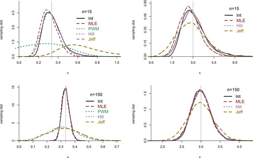
We carry out a simulation study to compare the calibration efficiency of the BRI, the ML and PWM estimators and present results on the shape parameter only for brevity. As the MHA is itself a time-consuming simulation process, it has been left out of this comparison. We generate 10,000 samples of size n = 15, 50, 100, from a Pareto distribution, $\text{Pa}(x|\kappa ,\sigma )$ – which is linked to the GPD as described in Section 1 – with σ = 4 and $\kappa =1/3,3,7.$ The parameters are calibrated using the BRI, ML, and PWM approaches, their sampling distribution are estimated, and their bias and mean-squared error (MSE) used as efficiency measures, illustrated in Table 1.

Table 1. Comparing estimators of the shape parameter. First four columns show the relative MSE to the MLE and the rest the bias of the ML, PWM, BRI, Jeffreys, and Hill estimators of the shape parameter, κ, from 5,000 samples of sizes n = 15, 50, 150 and $\kappa =1/3,3,7,$ with scale σ = 4 in all cases.

		relative MSE				Bias
n	κ	PWM	BRI	Jeff	Hill	MLE	PWM	BRI	Jeff	Hill
15	1/3	18.851	1.333	45.301	1.062	–0.024	–0.177	0.014	–0.086	–0.002
50		15.165	1.153	20.489	1.019	–0.007	–0.058	0.004	–0.003	–0.0002
150		16.169	1.028	16.369	1.006	–0.002	–0.023	0.001	0.436	–0.0002
15	3	7.673	1.366	1.914	1.065	–0.209	–2.148	0.124	2.556	–0.010
50		22.767	1.060	1.809	1.017	–0.066	–2.043	0.031	–0.041	0.006
150		65.431	1.011	1.793	1.011	–0.014	–2.014	0.012	–0.007	0.006
15	7	10.966	1.320	1.338	1.070	–0.478	–6.077	0.262	–0.143	–0.012
50		36.560	1.086	1.319	1.026	–0.121	–6.020	0.078	–0.020	0.020
150		111.657	1.096	1.325	1.005	–0.052	–6.006	0.031	–0.017	–0.005

Given that PWM works well only if (at least) the first two moments of the distribution exist it is not striking to confirm its poor performance for values of $\kappa \notin (-0.2,0.2)$ (Hosking, Wallis, and Wood 1985), regardless of the sample size. In contrast, both MLE and BRI estimators yield relatively low bias and MSE, even for moderate sample sizes, with their sampling distributions becoming increasingly similar as the sample size grows (Figure 1). Both estimators are invariant under one-to-one transformations, while PWM is not; further, BRI credible intervals are invariant, a feature we will exploit in the sequel.

Figure 1. Sampling distributions of the BRI, ML, PWM, and Jeffreys posterior median estimators of the shape parameter, from 5,000 simulations of sample sizes n = 15 (top), and n = 150 (bottom). Right panels display the case κ = 3 and left when $\kappa =1/3$ (marked by the vertical line). The right panels do not display PWM due to its poor performance. Note the MLE, BRI, and Hill estimators have relatively similar sampling distributions and are almost indistinguishable for large n.

5. Bank equity capital requirements

We apply the calibration approaches described above to equity risk capital that banks are required to hold in the banking Basel II regulations. In the Basel II regulations in pghs.700 and 718 (LXXVI)¹ a value-at-risk ($\text{VaR}$) approach is required for a 99th percentile one-sided confidence interval on 10-day equity returns. This means a bank will estimate what it thinks the 99th percentile 10-day equity returns can fall by (e.g., it might estimate this as a 10% fall in its equities market value) and it is then required to hold at least this amount as a monetary capital amount on its balance sheet to demonstrate the bank can withstand a 99th percentile fall in the value of its equities.

The regulations mention a number of approaches are possible to calculate this VAR and in this case study, a GPD is fitted to an historic time series of an equity index of 10-day returns. The equity index used here is the FTSE 100 index taken from yahoo finance 2/4/1984—26/7/2013².

The raw data have been pre-processed to convert the daily index values into 10-day returns, y_t (i.e., the percentage change in value of the index over non overlapping 10-day periods). A common question is either to use simple returns, $y_t=x_{t+10}/x_t-1$ where x_t is the index value at time t, or log-returns, $y_t=\hspace{0.17em}\text{log}\hspace{0.17em}(x_{t+10}/x_t).$ While the difference between these two definitions is not crucial for a 10-day period, the log returns have been used in this case study. This is because the left tail is of interest and is unbounded for the log return, but bounded at −100% for the simple return. An unbounded domain is potentially more appropriate for the GPD calibration. When the 99th percentile has been calibrated in log returns, this needs to be converted back to a simple return for the VAR value. For example, if an −11% fall in equity values is the log-return 99th percentile, this is a $\text{exp}\hspace{0.17em}(-0.11)-1=-0.104$ simple return fall in equity market value.

5.1. Exploratory data analysis

We explore some basic features of the data, presented for both simple and log returns on the left panel of Figure 2.

Figure 2. On the left panel, smoothed histograms of simple and log 10-day returns of the FTSE100 index from 2/4/84–26/7/13. Both distributions are almost identical, left skew with heavy tails, and present a small secondary mode on the left hand tail. On the right panel, mean excess function of the negative 10-day returns of the FTS100 (solid) with 95% confidence intervals (segmented). The positive slope suggests a heavy tail, amenable to a power distribution.

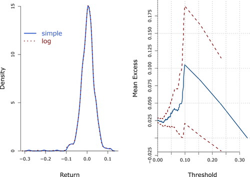
We would like to highlight that the distribution of the returns is fat tailed – it has a higher frequency of extreme events compared with a Gaussian distribution – as measured by its kurtosis (that of a Gaussian distribution is 3). It is also negatively skewed – a higher proportion on events are on the left-hand side of the mean, which emphasizes the underlying financial risks. Plotting the Mean Excess (ME) function, $M(u)=\mathbb{E}[X-u|x>u],$ is often used to explore whether the data have power tails (Ghosh and Resnick 2010). A characteristic of a fat-tailed GPD type distribution with negative shape parameter is an increasing straight line, while a decreasing line indicates thin tails; a horizontal line suggests exponential tails. The right panel in Figure 2 shows the mean excess plot of the absolute value of the negative log returns, which displays a positive slope (up to losses of about 10%), suggesting a power distribution is appropriate for this data. Combining this features with Figure 3 suggest a GPD with a negative shape parameter may be appropriate to model the negative returns of this dataset.

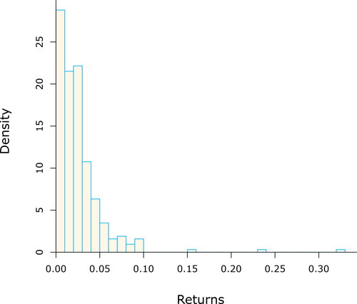
Figure 3. Histogram of the left tail of the 10-day log-returns from the FTSE100 data (in absolute value). The shape shows a power decay and heavy tails, with some extreme events, suggesting a GPD may be a suitable model.

5.2. Peaks over threshold

We now apply the calibration approaches described in Sections 2.1 and 3 to the left tail of the 10-day FTSE100 log returns, using the peaks over threshold approach (McNeil, Frey, and Embrechts 2005, with theory as in Section 1.1.2), which allows the focus to be on the percentiles of interest.

We do not discuss how to set the threshold, but refer the reader to de Zea Bermudez and Kotz (2010b). McNeil, Frey, and Embrechts (2005, 280) suggest using the ME plot as a guide to threshold setting. We subjectively pick −5% as the approximate point on the mean excess plot beyond which the slope appears to increase faster and end up with n = 33. It is noted there are still enough points beyond this level for reasonable calibration and the threshold is expected to be sufficiently high for the Picklands-Balkema-de Haan theorem to apply.

Relying on the fact that if $x\sim \text{gPa}(x|-1/\alpha ,\beta /\alpha ),$ then $y=1/x\sim \text{iPa}(y|\alpha ,1/\beta ),$ we use the methods in Section 2.1 to obtain point and interval estimates of the shape parameter. The MLE is straightforward to obtain, $\widehat{\kappa }=\hspace{0.17em}\text{log}\hspace{0.17em}(\widehat{\beta }/t)=2.44,$ where $t={\prod }_{i=1}^n{y}_i^{1/n},$ is the geometric mean and $\widehat{\beta }=\max \{y_1,\dots ,y_n\}=19.71$ is the MLE of the shape. 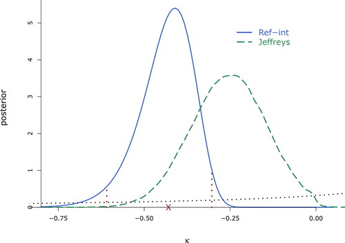The marginal posterior distribution of the shape parameter is $\text{Ga}(\kappa |n-1,n/\widehat{\kappa }),$ and the BRI point estimate ${\kappa }^{\ast }=2.33$ and interval $(1.642,3.298)$ are illustrated in Figure 4. In particular, notice the intrinsic interval is different from the HPD, $(1.573,3.195),$ highlights the fact that HPDs are not invariant under transformations, while the intrinsic is. Given that the scale parameter typically is a nuisance parameter, we use the analytical approximation to the BRI estimator, ${\sigma }^{\ast }\approx 2^{\frac{1}{n\widehat{\kappa }}}=19.88.$

Figure 4. Marginal posterior distribution of the shape parameter from the FTSE100 data, thresholded at –5%. Marked are the BRI estimate, ${\kappa }^{\ast }=-0.429,$ and interval, $(-0.609,-0.303).$ The (proper) marginal Jeffreys prior is represented by the dotted line, and the corresponding equally tailed interval of probability 0.95 is $(-0.472,-0.051).$

We use quasi-Newton (Fletcher and Reeves 1964) to maximize the likelihood for the GPD, yielding MLEs $\widehat{\kappa }=-0.380$ and $\widehat{\sigma }=0.0222.$ The confidence intervals are found from the observed covariance matrix, which gives a standard errors for $\widehat{\kappa }$ of 0.228; thus, an approximate 95% confidence interval for the shape is $(-0.828,0.0679).$ Using PWM, one gets $\tilde{\kappa }=-0.369$ and $\tilde{\sigma }=0.0224,$ with $(-0.844,0.106)$ a CI of approximate 95% for κ. Exploiting the invariance of the BRI estimator, ${\kappa }^{\ast }=-0.429$ and $(-0.609,-0.303)$ the BRI interval of probability 0.95. To fit the Bayesian model with Jeffreys prior, we generated chains of length 10⁶, dropped the first 10⁴ as burn-in and thinned every fifth draw, ending up with samples of size 198,000 for inference, the marginal posterior distributions are illustrated in Figure 4. The posterior mean and median of the shape are −0.254 and −0.252, respectively, and the equally tailed interval of posterior probability 0.95 is $(-0.472,-0.048).$ Note both frequentist CIs include 0, suggesting an exponential tail behavior, while the Bayesian alternatives strongly support heavy tails; also notice the intrinsic posterior has a smaller variance; hence, the BRI interval is shorter than the equally tailed from Jeffreys prior.

The Pareto principle and Gini index discussed in Section 1.2 depend only on the shape parameter, so we can use the invariance of the BRI and MLE approaches to calculate point and interval estimates shown in Table 2. As the calibration of the GPD is based on the tail of the data, we exploit its lack of memory to calculate $${\text{VaR}}_{\epsilon }=u+\frac{\sigma }{\kappa }(1-{\left(\frac{1-\epsilon }{\tilde{F}(u)}\right)}^k)$$ where u = 0.05 is the threshold and $\tilde{F}(u)$ is empirically estimated as the proportion of data points above the threshold relative to total number of data points (McNeil, Frey, and Embrechts 2005, 283); in our case $\tilde{F}(u)=33/316.$

Table 2. Point and interval estimates for the FTSE100 returns data, from the four approaches. The middle point in the intervals is the corresponding point estimate. Confidence intervals are of approximate 95%, and Bayesian credible intervals of probability 0.95. The point estimate from Jeffreys prior is the posterior median.

	κ	Gini index	${\text{VaR}}_{0.99}\%$
BRI	$(-0.609,-0.429,-0.303)$	$(0.589,0.637,0.719)$	10.42
Jeffreys	$(-0.472,-0.253,-0.051)$	$(0.513,0.573,0.654)$	9.27
ML	$(-0.828,-0.380,0.068)$	$(0.484,0.617,0.853)$	9.99
PWM	$(-0.844,-0.403,0.106)$	$(0.475,0.613,0.865)$	9.04

It is worth noticing both frequentist approaches do not rule out κ = 0, while the Bayesian alternatives strongly suggest $\kappa <0;$ all point estimates are negative, nonetheless. The posterior distribution from the intrinsic approach is shifted to the right, compared with the Jeffreys alternative and has a smaller variance. Frequentist confidence intervals are wider than the Bayesian credible counterparts.

This case study shows a practical example of how all four approaches can be used to calibrate the GPD. While there are some differences between the results from the four approaches, all point estimates of VaR0.99 are roughly similar, suggesting a level between 9% and 10% for regulatory equity capital might appropriately meet the Basel II regulations.

The BRI yields the highest VAR0.99 of the four methods, which would in practice mean holding more capital, but has the tightest intervals. Hence, although the point estimate may be seem marginally more costly, the level of uncertainty around it is much smaller, indeed reducing the risk associated with loss protection.

Point estimates of the shape and scale parameters (not shown) are roughly similar for each calibration approach, barring Jeffreys, which shrinks the estimate toward the origin; however, the length of the interval Bayesian estimates is shorter than their frequentist counterparts. Moreover, frequentist interval estimates for VaR0.99 are difficult to get and rely on asymptotic approximations, while those from BRI are immediate to obtain due to its invariance and those from Jeffreys prior are straightforward from the MCMC output.

6. Final remarks

We have illustrated how the BRI approach can be used to calibrate the GPD by using a transformation from the inverted-Pareto distribution. Four different approaches to calibrating the GPD have been presented. Three of the approaches were compared in a simulation study of simulated data from a Pareto distribution. All four approaches were then compared for similarities and differences in a case study.

From the simulation study, it is apparent that the repeated sampling behavior of the PWM estimator is poor in general and some modification is needed if it is to work in practice (see e.g., Chen et al. 2017). The results also indicate the BRI estimator has a similar MSE to the MLE even for moderated sample size, and its sampling distribution is asymptotically Gaussian (Figure 1 and Table 1).

Combined with its invariance under one-to-one transformations, it is a compelling alternative for calibration. One limitation of this simulation study was that it only simulated data from a Pareto distribution. An extension might be to compare the calibration approaches for data simulated from other distributions.

The BRI approach has produced lower mean-squared errors in the simulation studies, suggesting it to be more accurate for parameter estimation when the data are indeed from a Pareto distribution. The MLE is relatively simple to understand and implement; however, there are questions over the convergence of the numerical optimization methods, especially with fewer data points (de Zea Bermudez and Kotz 2010a). The PWM is likewise simple to understand and implement, but is efficient only for a subset of the parameter space and it could produce estimates with a likelihood of zero.

The MHA was left out of the simulation study as it is computationally intense. The results in Section 5.2 were obtained by running one million simulations. It would not be possible to run to this level of accuracy and carry out an outer layer 1000 simulation analysis in a reasonable time period or without much greater computer power. Also, implementing the sampler has a number of practical issues that are different for each dataset, which may take time to resolve and ensure the MHA converges in a reasonable time period. However, our implementation is robust and may be used as an off-the-shelf option.

One area of interest that could be the subject of further work is how sensitive the results are to the threshold used for each calibration method. A study might repeat the analysis looking at various different thresholds and how that impacts the shape, scale, and ${\text{VaR}}_{0.99}$ for each threshold.

Another area of potential interest is how the time period of each data point impacts the shape parameter and GPD calibrations. For example, if the case study looked at equity returns over 1 day, 5 days, 1 year, etc. What would the impact be on the GPD calibration? Clearly, a large time step for each data point would be expected to give higher values for the 99th percentile, but would the Gini index remain invariant to other size time steps as for the 10-day period investigated in this case study?

Notes

1 http://www.bis.org/publ/bcbs128b.pdf

2 Available from http://uk.finance.yahoo.com/q/hp?s=5EFTSE

Appendix A:

A literature on GPD estimation and its applications

Table A1. Some literature on GPD calibration approaches to datasets. Abbreviations are Maximum Literature (MLE), Method of Moments (MoM), Method of Medians (MM), Probability Weighted Moments (PWM), Elemental Percentile Method (EPM), Optimal Bias Robust Estimator (OBRE), Least Squares (LS), Maximum Entropy (ME), Minimum density power divergence estimator (MDPD).

Reference	Area of application	Calibration types used
Moharram, Gosain, and Kapoor (1993)	Hydrology	MOM, PWM, MLE, LS
Castillo and Hadi (1997)	Hydrology	MOM, PWM, EPM
McNeil (1997)	Insurance	MLE
Rootzén and Tajvidi (1997)	Insurance	PWM, MLE
Dupuis and Tsao (1998)	Hydrology	OBRE
Holmes and Moriarty (1999)	Weather	LS to the empirical mean excess function
Shi et al. (1999)	Engineering	MLE
Peng and Welsh (2001)	Hydrology	MM, MLE, OBRE
Pandey, Van Gelder, and Vrijling (2001)	Weather	L-moments, MoM
Frigessi, Haug, and Rue (2002)	Insurance	MLE
Diebolt, Guillou, and Worms (2003)	Hydrology	Bayesian and MLE
de Zea Bermudez and Turkman (2003)	Insurance, Hydrology	Bayesian, PWM and EPM
Pisarenko and Sornette (2003)	Seismology	MLE
Coles, Pericchi, and Sisson (2003)	Weather	Bayesian and MLE
Castillo et al. (2004)	Engineering	MOM, PWM, EPM
La Cour (2004)	Engineering	MLE
Engeland, Hisdal, and Frigessi (2004)	Hydrology	PWM, MLE
Behrens, Lopes, and Gamerman (2004)	Economics	Bayesian, ML
Pandey, Van Gelder, and Vrijling (2004)	Hydrology	L-Moments, MoM
Juárez and Schucany (2004)	Weather	MM, OBRE, MLE, MDPD
Goldstein, Morris, and Yen (2004)	Network theory	MLE, LS
Keylock (2005)	Environment	MLE
Diebolt et al. (2005)	Insurance	Bayesian, MLE
Öztekin (2005)	Hydrology	MOM, PWM. MLE, LS, ME
Tancredi, Anderson, and O’Hagan (2006)	Hydrology	Bayesian
Lana et al. (2006)	Weather	L-moments
Jagger and Elsner (2006)	Weather	Bayesian and MLE
Fawcett and Walshaw (2006)	Weather	Bayesian and MLE
Zagorski and Wnek (2007)	Engineering	MLE, LS to empirical mean excess function
Castellanos and Cabras (2007)	Hydrology	Bayesian and MLE
Moisello (2007)	Hydrology, Weather	PWM
Vilar-Zanón and Lozano-Colomer (2007)	Insurance	Bayesian
White, Enquist, and Green (2008)	Ecology	MLE, binning
Krehbiel and Adkins (2008)	Economics	MLE
de Zea Bermudez et al. (2009)	Wildfires	PWM, MLE
Mendes et al. (2010)	Wildfires	Bayesian
Akhundjanov and Chamberlain (2019)	Agricultural land size	MLE, Hill and KS

References

- Akhundjanov, S. B., and L. Chamberlain. 2019. The power-law distribution of agricultural land size. Journal of Applied Statistics 46 (16):3044–56. doi:10.1080/02664763.2019.1624695.
- Behrens, C. N., H. F. Lopes, and G. Gamerman. 2004. Bayesian analysis of extreme events with threshold estimation. Statistical Modelling 4 (3):227–44. doi:10.1191/1471082X04st075oa.
- Beirlant, J., Y. Goegebeur, J. Teugels, and J. Segers. 2005. Statistics of Extremes: Theory and Applications. Chichester: Springer.
- Beirlant, J., J. Teugels, and P. Vynckier. 1996. Practical analysis of extreme values. Leuven: University Press.
- Berger, J., J. M. Bernardo, and D. Sun. 2009. The formal definition of reference priors. The Annals of Statistics 37 (2):905–38. doi:10.1214/07-AOS587.
- Berger, J., J. M. Bernardo, and D. Sun. 2015. Overall objective priors. Bayesian Analysis 10 (1):189–221. doi:10.1214/14-BA915.
- Bernardo, J. M. 2007. Objective Bayesian point and region estimation in location-scale models. Statistics and Operations Research Transactions 31:3–44.
- Bernardo, J. M., and M. A. Juárez. 2003. Intrinsic estimation. Bayesian Statistics 7, eds. J. M. Bernardo, M. J. Bayarri, J. O. Berger, A. P. Dawid, D. Heckerman, A. F. M. Smith, and M. West, 465–76. Oxford: Oxford University Press.
- Bernardo, J. M., and R. Rueda. 2002. Bayesian hypothesis testing: A reference approach. International Statistical Review 70 (3):351–72. doi:10.1111/j.1751-5823.2002.tb00175.x.
- Castellanos, M. E., and S. Cabras. 2007. A default Bayesian procedure for the generalized Pareto distribution. Journal of Statistical Planning and Inference 137 (2):473–83. doi:10.1016/j.jspi.2006.01.006.
- Castillo, E., and A. S. Hadi. 1997. Fitting the generalized Pareto distribution to data. Journal of the American Statistical Association 92 (440):1609–20. doi:10.1080/01621459.1997.10473683.
- Castillo, E., A. S. Hadi, N. Balakrishnan, and J. M. Sarabia. 2004. Extreme value and related models with applications in engineering and science. New Jersey: Wiley.
- Charras-Garrido, M., and P. Lezaud. 2013. Extreme value analysis: An introduction. Journal de la Société Française de Statistique 154:66–97.
- Chen, H., W. Cheng, J. Zhao, and X. Zhao. 2017. Parameter estimation for generalized Pareto distribution by generalized probability weighted moment-equations. Communications in Statistics - Simulation and Computation 46 (10):7761–76. doi:10.1080/03610918.2016.1249884.
- Coles, S. 2001. An introduction to statistical modeling of extreme values. London: Springer-Verlag.
- Coles, S., L. R. Pericchi, and S. Sisson. 2003. A fully probabilistic approach to extreme rainfall modeling. Journal of Hydrology 273 (1–4):35–50. doi:10.1016/S0022-1694(02)00353-0.
- Davidson, A. C., and R. L. Smith. 1990. Models for exceedances over high thresholds. Journal of the Royal Statistical Society B 52:393–442.
- Diebolt, J., A. Guillou, and R. Worms. 2003. Asymptotic behaviour of the probability weighted moments and penultimate approximation. ESAIM: Probability and Statistics 7:219–38. doi:10.1051/ps:2003010.
- Diebolt, J., M. A. El-Aroui, M. Garrido, and S. Girard. 2005. Quasi-conjugate Bayes estimates for GPD parameters and application to heavy tails modelling. Extremes 8 (1–2):57–78. doi:10.1007/s10687-005-4860-9.
- Dupuis, D., and M. Tsao. 1998. A hybrid estimator for generalized Pareto and extreme-value distributions. Communications in Statistics - Theory and Methods 27 (4):925–41. doi:10.1080/03610929808832136.
- Embrechts, P., C. Klüppelberg, and T. Mikosch. 1997. Modelling extremal events. Berlin: Springer-Verlag.
- Engeland, K., H. Hisdal, and A. Frigessi. 2004. Practical extreme value modelling of hydrological floods and droughts: A case study. Extremes 7 (1):5–30. doi:10.1007/s10687-004-4727-5.
- Fawcett, L., and D. Walshaw. 2006. A hierarchical model for extreme wind speeds. Journal of the Royal Statistical Society: Series C (Applied Statistics) 55 (5):631–46. doi:10.1111/j.1467-9876.2006.00557.x.
- Fletcher, R., and C. M. Reeves. 1964. Function minimization by conjugate gradients. The Computer Journal 7 (2):149–54. doi:10.1093/comjnl/7.2.149.
- Frigessi, A., O. Haug, and H. Rue. 2002. A dynamic mixture model for unsupervised tail estimation without threshold selection. Extremes 5 (3):219–35. doi:10.1023/A:1024072610684.
- Galambos, J. 1987. The asymptotic theory of extreme order statistics, 2nd edn. New York: Wiley.
- Ghosh, S., and S. Resnick. 2010. A discussion on mean excess plots. Stochastic Processes and Their Applications 120 (8):1492–517. doi:10.1016/j.spa.2010.04.002.
- Gilleland, E., M. Ribatet, and A. C. Stephenson. 2013. A software review for extreme value analysis. Extremes 16 (1):103–19. doi:10.1007/s10687-012-0155-0.
- Goldstein, M. L., S. A. Morris, and G. G. Yen. 2004. Problems with fitting to the power-law distribution. The European Physical Journal B 41 (2):255–8. doi:10.1140/epjb/e2004-00316-5.
- Greenwood, J. A., J. M. Landwehr, N. C. Matalas, and J. R. Wallis. 1979. Probability weighted moments: Definition and relation to parameters of several distributions expressable in inverse form. Water Resources Research 15 (5):1049–54. doi:10.1029/WR015i005p01049.
- de Haan, L., and A. F. Ferreira. 2006. Extreme value theory: An introduction. New York: Springer.
- Hill, B. M. 1975. A simple general approach to inference about the tail of a distribution. The Annals of Statistics 3 (5):1163–74. doi:10.1214/aos/1176343247.
- Holmes, J., and W. Moriarty. 1999. Application of the generalized Pareto distribution to extreme value analysis in wind engineering. Journal of Wind Engineering and Industrial Aerodynamics 83 (1–3):1–10. doi:10.1016/S0167-6105(99)00056-2.
- Hosking, J. R. M., J. R. Wallis, and E. F. Wood. 1985. Estimation of the generalized extreme value distribution by the method of probability weighted moments. Technometrics 27 (3):251–61. doi:10.1080/00401706.1985.10488049.
- Jagger, T. H., and J. B. Elsner. 2006. Climatology models for extreme hurricane winds near the United States. Journal of Climate 19 (13):3220–36. doi:10.1175/JCLI3913.1.
- Juárez, S. F., and W. R. Schucany. 2004. Robust and efficient estimation for the generalized Pareto distribution. Extremes 7 (3):237–51. doi:10.1007/s10687-005-6475-6.
- Juárez, M. A. 2005. Objective Bayes estimation and hypothesis testing: The reference-intrinsic approach on non-regular models. CRISM Working Paper 05–14.
- Keylock, C. 2005. An alternative form for the statistical distribution of extreme avalanche runout distances. Cold Regions Science and Technology 42 (3):185–93. doi:10.1016/j.coldregions.2005.01.004.
- Koch, R. 2007. The 80/20 principle: The secret of achieving more with less. London: Nicholas Brealey Publishing.
- Kotz, S., and S. Nadarajah. 2000. Extreme value distributions: Theory and applications. London: Imperial College Press.
- Krehbiel, T., and L. C. Adkins. 2008. Extreme daily changes in U.S. dollar London inter-bank offer rates. International Review of Economics & Finance 17 (3):397–411. doi:10.1016/j.iref.2006.08.009.
- La Cour, B. R. 2004. Statistical characterization of active sonar reverberation using extreme value theory. IEEE Journal of Oceanic Engineering 29 (2):310–6. doi:10.1109/JOE.2004.826897.
- Lana, X., A. Burgueño, M. Martínez, and C. Serra. 2006. Statistical distributions and sampling strategies for the analysis of extreme dry spells in Catalonia (NE Spain). Journal of Hydrology 324 (1–4):94–114. doi:10.1016/j.jhydrol.2005.09.013.
- Leadbetter, M. R., G. Lindgren, and H. Rootzen. 1983. Extremes and related properties of random sequences and processes. New York: Springer.
- Lima, C. H. R., U. Lall, T. Troy, and N. Devineni. 2016. A hierarchical Bayesian GEV model for improving local and regional flood quantile estimates. Journal of Hydrology 541:816–23. doi:10.1016/j.jhydrol.2016.07.042.
- Malik, H. J. 1970. Estimation of the parameters of a Pareto distribution. Metrika 15 (1):126–32. doi:10.1007/BF02613565.
- McNeil, A. J., R. Frey, and P. Embrechts. 2005. Quantitative risk management: Concepts, techniques and tools. Princeton: University Press.
- McNeil, A. J. 1997. Estimating the tails of loss severity distributions using extreme value theory. ASTIN Bulletin 27 (1):117–37. doi:10.2143/AST.27.1.563210.
- Mendes, J. M., P. C. de Zea Bermudez, J. Pereira, K. F. Turkman, and M. J. P. Vasconcelos. 2010. Spatial extremes of wildfire sizes: Bayesian hierarchical models for extremes. Environmental and Ecological Statistics 17 (1):1–28. doi:10.1007/s10651-008-0099-3.
- Moharram, S. H., A. K. Gosain, and P. N. Kapoor. 1993. A comparative study for the estimators of the generalized Pareto distribution. Journal of Hydrology 150 (1):169–85. doi:10.1016/0022-1694(93)90160-B.
- Moisello, U. 2007. On the use of partial probability weighted moments in the analysis of hydrological extremes. Hydrological Processes 21 (10):1265–79. doi:10.1002/hyp.6310.
- Öztekin, T. 2005. Comparison of parameter estimation methods for the three-parameter generalized Pareto distribution. Turkish Journal of Agriculture and Forestry 29:419–28.
- Pandey, M. D., P. H. A. J. M. Van Gelder, and J. K. Vrijling. 2001. The estimation of extreme quantiles of wind velocity using L-moments in the peaks-over-threshold approach. Structural Safety 23 (2):179–92. doi:10.1016/S0167-4730(01)00012-1.
- Pandey, M. D., P. H. A. J. M. Van Gelder, and J. K. Vrijling. 2004. Dutch case studies of the estimation of extreme quantiles and associated uncertainty by bootstrap simulations. Environmetrics 15 (7):687–99. doi:10.1002/env.656.
- Peng, L., and A. Welsh. 2001. Robust estimation of the generalized Pareto distribution. Extremes 4 (1):53–65. doi:10.1023/A:1012233423407.
- Persky, J. 1992. Retrospectives: Pareto’s law. Journal of Economic Perspectives 6 (2):181–92. doi:10.1257/jep.6.2.181.
- Pickands, J. 1975. Statistical inference using extreme order statistics. The Annals of Statistics 3:119–31.
- Pisarenko, V. F., and D. Sornette. 2003. Characterization of the frequency of extreme earthquake events by the generalized Pareto distribution. Pure and Applied Geophysics 160 (12):2343–64. doi:10.1007/s00024-003-2397-x.
- R Core Team. 2021. R: A language and environment for statistical computing. Vienna: R Foundation for Statistical Computing. https://www.R-project.org/
- Ragulina, G., and T. Reitan. 2017. Generalized extreme value shape parameter and its nature for extreme precipitation using long time series and the Bayesian approach. Hydrological Sciences Journal 62 (6):863–79. doi:10.1080/02626667.2016.1260134.
- Robert, C. P. 1996. Intrinsic losses. Theory and Decision 40 (2):191–214. doi:10.1007/BF00133173.
- Rootzén, H., and N. Tajvidi. 1997. Extreme value statistics and wind storm losses: A case study. Scandinavian Actuarial Journal 1997 (1):70–94. doi:10.1080/03461238.1997.10413979.
- Rytgaard, M. 1990. Estimation in the Pareto distribution. ASTIN Bulletin 20 (2):201–16. doi:10.2143/AST.20.2.2005443.
- Shi, G., H. Atkinson, C. Sellars, and C. Anderson. 1999. Application of the generalized Pareto distribution to the estimation of the size of the maximum inclusion in clean steels. Acta Materialia 47 (5):1455–68. doi:10.1016/S1359-6454(99)00034-8.
- Tancredi, A., C. Anderson, and A. O’Hagan. 2006. Accounting for threshold uncertainty in extreme value estimation. Extremes 9 (2):87–106. doi:10.1007/s10687-006-0009-8.
- Vilar-Zanón, J. L., and C. Lozano-Colomer. 2007. On Pareto conjugate priors and their application to large claims reinsurance premium calculation. ASTIN Bulletin 37 (2):405–28. doi:10.1017/S0515036100014938.
- White, E. P., B. J. Enquist, and J. L. Green. 2008. On estimating the exponent of power-law frequency distributions. Ecology 89:905–12. doi:10.1890/07-1288.1.
- Zagorski, M., and M. Wnek. 2007. Analysis of the turbine steady-state data by means of generalized Pareto distribution. Mechanical Systems and Signal Processing 21 (6):2546–59. doi:10.1016/j.ymssp.2007.01.002.
- de Zea Bermudez, P., and S. Kotz. 2010a. Parameter estimation of the generalized Pareto distribution–Part I. Journal of Statistical Planning and Inference 140 (6):1353–73. doi:10.1016/j.jspi.2008.11.019.
- de Zea Bermudez, P., and S. Kotz. 2010b. Parameter estimation of the generalized Pareto distribution–Part II. Journal of Statistical Planning and Inference 140 (6):1374–88. doi:10.1016/j.jspi.2008.11.020.
- de Zea Bermudez, P., J. Mendes, J. M. C. Pereira, K. F. Turkman, and M. J. P. Vasconcelos. 2009. Spatial and temporal extremes of wildfire sizes in Portugal (1984–2004). International Journal of Wildland Fire 18 (8):983–91. doi:10.1071/WF07044.
- de Zea Bermudez, P., and M. A. A. Turkman. 2003. Bayesian approach to parameter estimation of the generalized Pareto distribution. Test 12 (1):259–77. doi:10.1007/BF02595822.