Coordinate optimization for generalized fused Lasso

Abstract

Fused Lasso is one of extensions of Lasso to shrink differences of parameters. We focus on a general form of it called generalized fused Lasso (GFL). The optimization problem for GFL can be came down to that for generalized Lasso and can be solved via a path algorithm for generalized Lasso. Moreover, the path algorithm is implemented via the genlasso package in R. However, the genlasso package has some computational problems. Then, we apply a coordinate descent algorithm (CDA) to solve the optimization problem for GFL. We give update equations of the CDA in closed forms, without considering the Karush-Kuhn-Tucker conditions. Furthermore, we show an application of the CDA to a real data analysis.

Keywords:

• Coordinate descent algorithm
• generalized fused Lasso
• generalized Lasso

1. Introduction

Suppose that there are m groups and n_j pairs of data $\{y_{j,i},{\mathit{x}}_{j,i}\}(i=1,\dots ,n_j)$ are observed for group $j\in \{1,\dots ,m\},$ where $y_{j,i}$ is a response variable and ${\mathit{x}}_{j,i}$ is a p-dimensional vector of non stochastic explanatory variables. Let ${\mathit{y}}_j$ be an n_j-dimensional vector defined by ${\mathit{y}}_j=(y_{j,1},\dots ,y_{j,n_j})\prime$ and ${\mathit{X}}_j$ be an $n_j\times p$ matrix defined by ${\mathit{X}}_j=({\mathit{x}}_{j,1},\dots ,{\mathit{x}}_{j,n_j})\prime .$ For group j, we consider the following linear regression model: (1) $${\mathit{y}}_j={\mathit{X}}_j\mathit{\beta }+{\mu }_j{\mathit{1}}_{n_j}+{\mathit{\epsilon }}_j,$$(1) where $\mathit{\beta }$ is a p-dimensional vector of regression coefficients, μ_j is a location parameter for group j, ${\mathit{1}}_n$ is an n-dimensional vector of ones, and ${\mathit{\epsilon }}_j$ is an n_j-dimensional vector of error variables from a distribution with mean 0 and variance ${\sigma }^2.$ In addition, we assume that the vectors ${\mathit{\epsilon }}_1,\dots ,{\mathit{\epsilon }}_m$ are independent. Let $\mathit{y}$ be an n-dimensional vector defined by $\mathit{y}=({\mathit{y}}_1^{\prime },\dots ,{\mathit{y}}_m^{\prime })\prime ,\mathit{X}$ be an n × p matrix defined by $\mathit{X}=({\mathit{X}}_1^{\prime },\dots ,{\mathit{X}}_m^{\prime })\prime ,\mathit{\mu }$ be an m-dimensional vector defined by $\mathit{\mu }=({\mu }_1,\dots ,{\mu }_m)\prime ,\mathit{R}$ be an $n\times m$ block diagonal matrix defined by $\mathit{R}=\mathit{d}\mathit{iag}({\mathit{1}}_{n_1},\dots ,{\mathit{1}}_{n_m}),$ and $\mathit{\epsilon }$ be an n-dimensional vector defined by $\mathit{\epsilon }=({\mathit{\epsilon }}_1^{\prime },\dots ,{\mathit{\epsilon }}_m^{\prime })\prime ,$ where $n={\sum }_{j=1}^m{n}_j.$ Then, m models in (1)(1) $${\mathit{y}}_j={\mathit{X}}_j\mathit{\beta }+{\mu }_j{\mathit{1}}_{n_j}+{\mathit{\epsilon }}_j,$$(1) are expressed as $$\mathit{y}=\mathit{X\beta }+\mathit{R\mu }+\mathit{\epsilon }.$$

In this paper, although we deal with a linear regression model, we consider the case that location parameters of the model are different for each groups, that is, it can be regarded that location parameters express individual effects of groups. We call μ_j group effect for group j. In such case, one of interesting points is which group effects are equivalence. Hence, we approach it by using penalized least square method. That is, $\mathit{\mu }$ is estimated by minimizing the following penalized residual sum of squares (PRSS): (2) $$\Vert \mathit{y}-\mathit{X\beta }-\mathit{R\mu }{\Vert }_2^2+\lambda \sum _{j=1}^m\sum _{\mathcal{\ell }\in D_j}{w}_{j\mathcal{\ell }}|{\mu }_j-{\mu }_{\mathcal{\ell }}|,$$(2) where λ is a positive tuning parameter, $D_j\subset \{1,\dots ,m\}\backslash \left\{j\right\}$ is an index set, and $w_{j\mathcal{\ell }}$ is a positive weight satisfying $w_{j\mathcal{\ell }}=w_{\mathcal{\ell }j}.$ This is called generalized fused Lasso (GFL). The original form of GFL was proposed by Tibshirani et al. (2005) and is called fused Lasso (FL). When $D_1=\varnothing ,D_j=\{j-1\}(j=2,\dots ,m),$ and $w_{j\mathcal{\ell }}=1,$ GFL coincides with FL. GFL shrinks $|{\mu }_j-{\mu }_{\mathcal{\ell }}|$ toward 0 and the estimates of μ_j and ${\mu }_{\mathcal{\ell }}$ are often equal. Hence, using GFL, we can identify groups with equal group effects.

To obtain the GFL estimator of $\mathit{\mu },$ we need an optimization method to minimize (2)(2) $$\Vert \mathit{y}-\mathit{X\beta }-\mathit{R\mu }{\Vert }_2^2+\lambda \sum _{j=1}^m\sum _{\mathcal{\ell }\in D_j}{w}_{j\mathcal{\ell }}|{\mu }_j-{\mu }_{\mathcal{\ell }}|,$$(2) . For FL, Friedman et al. (2007) proposed a coordinate descent algorithm (CDA). In other cases, the optimization problem can be came down to that of the ordinary Lasso (Tibshirani 1996) under some conditions (e.g., Sun, Wang, and Fuentes 2016; Li and Sang 2019). In this paper, we deal with the case that the above methods cannot be applied. That is, we assume that ${\sum }_{j=1}^m\#(D_j)>m.$ Fortunately, GFL can be expressed as generalized Lasso (Tibshirani and Taylor 2011). Generalized Lasso type penalty is given by $\Vert \mathit{D\mu }{\Vert }_1,$ where $\mathit{D}$ is a penalty matrix. For FL, $\mathit{D}$ is an $(m-1)\times m$ matrix given by $$\mathit{D}=\left(\begin{array}{ccccc}-1& 1& 0& \cdots & 0\\ 0& \ddots & \ddots & \ddots & ⋮\\ ⋮& \ddots & \ddots & \ddots & 0\\ 0& \cdots & 0& -1& 1\end{array}\right).$$

In addition, Tibshirani and Taylor (2011) proposed the optimization algorithm for generalized Lasso and the algorithm is implemented via the genlasso package (e.g., Arnold and Tibshirani 2019) in R (e.g., R Core Team 2019). However, the optimization with the genlasso package has a high calculation cost and cannot be practically executed in large sample data. Moreover, there are issues in terms of numerical error and estimates cannot be exactly equal. Accordingly, we focus on a CDA.

To accurately calculate the GFL estimator of $\mathit{\mu },$ even in large sample data, we give update equations of the CDA in closed form. Our algorithm has advantages compared with several existing algorithms, for example, by Friedman et al. (2007) and Tibshirani and Taylor (2011). Their algorithms are via Lagrange dual problem and must consider several conditions, for example, Karush-Kuhn-Tucker conditions and optimality. On the other hand, using our algorithm, the optimization problem for GFL can be solved by elementary mathematics, without considering these conditions. Moreover, although our algorithm reduces a search range of the minimizer for the jth coordinate direction to $2\#(D_j)+1$ discrete points that are given by closed forms, a numerical search like comparing values for each point in the reduced search range is not required. By checking simple conditions, the unique minimizer for a coordinate direction can be decided. Of course, the unique minimizer is given by closed form and ensures minimization for coordinate direction.

The remainder of the paper is organized as follows: In Section 2, we give closed form update equations of the CDA for GFL. Numerical examples are discussed in Section 3. Section 4 is conclusion of this paper. Technical details are provided in the Appendix.

2. Main results

We derive update equations of the CDA for obtaining the GFL estimator of $\mathit{\mu }.$ A CDA updates a solution along coordinate directions. The CDA for FL consists of a descent cycle and a fusion cycle. The descent cycle successively minimizes along coordinate directions. The ordinary CDA only consists of the descent cycle. However, when the ordinary CDA is applied for FL, some estimates are equal and then the solution gets stuck, failing to reach the minimum. To avoid this problem, Friedman et al. (2007) invoked the fusion cycle. Since this problem can also occur for GFL, we give update equations for the descent cycle and the fusion cycle. In this section, we regard that $\mathit{\beta }$ is fixed at $\mathit{\beta }=\widehat{\mathit{\beta }},$ and minimize the following PRSS: (3) $$\Vert \tilde{\mathit{y}}-\mathit{R\mu }{\Vert }_2^2+\lambda \sum _{j=1}^m\sum _{\mathcal{\ell }\in D_j}{w}_{j\mathcal{\ell }}|{\mu }_j-{\mu }_{\mathcal{\ell }}|,$$(3) where $\tilde{\mathit{y}}=\mathit{y}-\mathit{X}\widehat{\mathit{\beta }}.$

2.1. Descent cycle

The descent cycle minimizes along coordinate directions. That is, (3)(3) $$\Vert \tilde{\mathit{y}}-\mathit{R\mu }{\Vert }_2^2+\lambda \sum _{j=1}^m\sum _{\mathcal{\ell }\in D_j}{w}_{j\mathcal{\ell }}|{\mu }_j-{\mu }_{\mathcal{\ell }}|,$$(3) is minimized with respect to μ_i and repeat it for $i=1,\dots ,m.$ We fix ${\mu }_j(j\in \{1,\dots ,m\}\backslash \{i\})$ at ${\mu }_j={\widehat{\mu }}_j.$ Then, (3)(3) $$\Vert \tilde{\mathit{y}}-\mathit{R\mu }{\Vert }_2^2+\lambda \sum _{j=1}^m\sum _{\mathcal{\ell }\in D_j}{w}_{j\mathcal{\ell }}|{\mu }_j-{\mu }_{\mathcal{\ell }}|,$$(3) is rewritten as the function of μ_i by the following lemma (the proof is given in Appendix A):

Lemma 2.1.

The Equation (3)(3) $$\Vert \tilde{\mathit{y}}-\mathit{R\mu }{\Vert }_2^2+\lambda \sum _{j=1}^m\sum _{\mathcal{\ell }\in D_j}{w}_{j\mathcal{\ell }}|{\mu }_j-{\mu }_{\mathcal{\ell }}|,$$(3) can be expressed as the following function of ${\mu }_i(i\in \{1,\dots ,m\})$: (4) $$n_i{\mu }_i^2-2{\tilde{\mathit{y}}}_i^{\prime }{\mathit{1}}_{n_i}{\mu }_i+2\lambda \sum _{j\in D_i}{w}_{ij}|{\mu }_i-{\widehat{\mu }}_j|+u_i,$$(4) where ${\tilde{\mathit{y}}}_i$ is the ith block of $\tilde{\mathit{y}}$, that is, ${\tilde{\mathit{y}}}_i={\mathit{y}}_i-{\mathit{X}}_i\widehat{\mathit{\beta }}$ and u_i is the term that does not depend on μ_i.

From Lemma 2.1, essentially, it is sufficient to minimize the following function: (5) $$\varphi (x)=c_2{x}^2-2c_{1}x+2\lambda \sum _{j=1}^r{w}_j|x-b_j|\hspace{1em}(c_2,w_1,\dots ,w_r>0).$$(5)

Let $t_0=-\infty$ and let $t_1,\dots ,t_r$ be the order statistics of $b_1,\dots ,b_r,$ that is, $$t_j=\{\begin{array}{cc}\min \{b_1,\dots ,b_r\}\hfill & (j=1)\hfill \\ \min \left\{\{b_1,\dots ,b_r\}\backslash \{t_1,\dots ,t_{j-1}\}\right\}\hfill & (j=2,\dots ,r)\hfill \end{array},$$ $J_a^{+}$ and $J_a^{-}$ be index sets for $a\in \{0,1,\dots ,r\}$ defined by $$J_a^{+}=\left\{j\in \{1,\dots ,r\}\mid b_j\le t_a\right\},\hspace{1em}{J}_a^{-}=\left\{j\in \{1,\dots ,r\}\mid b_j>t_a\right\},$$ and R_a be a range defined by $$R_a=\{\begin{array}{cc}(t_a,t_{a+1}]\hfill & (a=0,1,\dots ,r-1)\hfill \\ (t_r,\infty )\hfill & (a=r)\hfill \end{array}.$$

Moreover, we define ${\tilde{w}}_a$ and v_a for $a\in \{0,1,\dots ,r\}$ as $${\tilde{w}}_a=\sum _{j\in J_a^{+}}{w}_j-\sum _{j\in J_a^{-}}{w}_j,\hspace{1em}{v}_a=\frac{c_1-\lambda {\tilde{w}}_a}{c_2}.$$

Then, the minimizer of (5)(5) $$\varphi (x)=c_2{x}^2-2c_{1}x+2\lambda \sum _{j=1}^r{w}_j|x-b_j|\hspace{1em}(c_2,w_1,\dots ,w_r>0).$$(5) is given by the following theorem (the proof is given in Appendix B):

Theorem 2.2.

Let $a^{\ast }$ and $a^{\star }$ be non negative values defined by $$a^{\ast }\in \{0,1,\dots ,r\}s.t.v_{a^{\ast }}\in R_{a^{\ast }},\hspace{1em}{a}^{\star }\in \{1,\dots ,r\}s.t.t_{a^{\star }}\in [v_{a^{\star }},v_{a^{\star }-1}).$$

Then, either $a^{\ast }$ or $a^{\star }$ uniquely exists, and the minimizer of $\varphi (x)$ in (5)(5) $$\varphi (x)=c_2{x}^2-2c_{1}x+2\lambda \sum _{j=1}^r{w}_j|x-b_j|\hspace{1em}(c_2,w_1,\dots ,w_r>0).$$(5) is given by $$\widehat{x}=\{\begin{array}{cc}{v}_{a^{\ast }}\hfill & (a^{\ast }\mathit{\text{exists}})\hfill \\ t_{a^{\star }}\hfill & (a^{\star }\mathit{\text{exists}})\hfill \end{array}.$$

Theorem 2.2

gives the unique minimizer of μ_i in (4)(4) $$n_i{\mu }_i^2-2{\tilde{\mathit{y}}}_i^{\prime }{\mathit{1}}_{n_i}{\mu }_i+2\lambda \sum _{j\in D_i}{w}_{ij}|{\mu }_i-{\widehat{\mu }}_j|+u_i,$$(4) . Hence, by applying Theorem 2.2 to (4)(4) $$n_i{\mu }_i^2-2{\tilde{\mathit{y}}}_i^{\prime }{\mathit{1}}_{n_i}{\mu }_i+2\lambda \sum _{j\in D_i}{w}_{ij}|{\mu }_i-{\widehat{\mu }}_j|+u_i,$$(4) for $i=1,\dots ,m,$ we can obtain the solution of $\mathit{\mu }$ in the descent cycle. In Theorem 2.2, when $a^{\star }$ exists, estimate of μ_i is equal to ${\widehat{\mu }}_j$ (satisfying ${\widehat{\mu }}_j=t_{a^{\star }}$), and this means that group effects of groups i and j are equal.

2.2. Fusion cycle

The fusion cycle avoids a solution getting stuck when some estimates are equal in the descent cycle. Suppose that we obtain ${\widehat{\mu }}_j={\widehat{\mu }}_{\mathcal{\ell }}$ as estimates of μ_j and ${\mu }_{\mathcal{\ell }}(j\ne \mathcal{\ell })$ in the descent cycle. Then, to avoid the solutions of μ_j and ${\mu }_{\mathcal{\ell }}$ getting stuck, we regard ${\eta }_i={\mu }_j={\mu }_{\mathcal{\ell }}$ and minimize (3)(3) $$\Vert \tilde{\mathit{y}}-\mathit{R\mu }{\Vert }_2^2+\lambda \sum _{j=1}^m\sum _{\mathcal{\ell }\in D_j}{w}_{j\mathcal{\ell }}|{\mu }_j-{\mu }_{\mathcal{\ell }}|,$$(3) along the η_i-axis direction.

After the descent cycle, suppose that we obtain ${\widehat{\mu }}_1,\dots ,{\widehat{\mu }}_m$ as estimates of ${\mu }_1,\dots ,{\mu }_m.$ Then, let ${\widehat{\eta }}_1,\dots ,{\widehat{\eta }}_b(b\le m)$ be distinct values of ${\widehat{\mu }}_1,\dots ,{\widehat{\mu }}_m$ and we define index sets $E_1,\dots ,E_b$ as $$E_j=\left\{\mathcal{\ell }\in \{1,\dots ,m\}\mid {\widehat{\mu }}_{\mathcal{\ell }}={\widehat{\eta }}_j\right\},$$ where $E_j\ne \varnothing$ and $E_j\cap E_{\mathcal{\ell }}=\varnothing (j\ne \mathcal{\ell }).$ If b < m, the fusion cycle is executed. In the fusion cycle, (3)(3) $$\Vert \tilde{\mathit{y}}-\mathit{R\mu }{\Vert }_2^2+\lambda \sum _{j=1}^m\sum _{\mathcal{\ell }\in D_j}{w}_{j\mathcal{\ell }}|{\mu }_j-{\mu }_{\mathcal{\ell }}|,$$(3) is minimized with respect to η_i and repeat it for $i\in \{j\in \{1,\dots ,b\}\mid \#(E_j)\ge 2\}.$ We fix ${\eta }_j(j\in \{1,\dots ,b\}\backslash \{i\})$ at ${\eta }_j={\widehat{\eta }}_j.$ Moreover, we define $D_j^{\ast }\subseteq \{1,\dots ,b\}\backslash \left\{j\right\}(j\in \{1,\dots ,b\})$ and $w_{j\mathcal{\ell }}^{\ast }(j\in \{1,\dots ,b\};\mathcal{\ell }\in D_j^{\ast })$ as $$\begin{array}{c}{D}_j^{\ast }=\left\{\mathcal{\ell }\in \{1,\dots ,b\}\backslash \backslash \left\{j\right\}\mid E_{\mathcal{\ell }}\cap F_j\ne \varnothing \right\},\hspace{1em}{F}_j=\underset{\mathcal{\ell }\in E_j}{\cup }{D}_{\mathcal{\ell }}\backslash E_j,\\ w_{j\mathcal{\ell }}^{\ast }=\sum _{(i,s)\in {\mathcal{J}}_{j\mathcal{\ell }}}{w}_{is},\hspace{1em}{\mathcal{J}}_{j\mathcal{\ell }}=\underset{i\in E_j}{\cup }\left\{i\right\}\times (E_{\mathcal{\ell }}\cap D_i).\end{array}$$

Then, (3)(3) $$\Vert \tilde{\mathit{y}}-\mathit{R\mu }{\Vert }_2^2+\lambda \sum _{j=1}^m\sum _{\mathcal{\ell }\in D_j}{w}_{j\mathcal{\ell }}|{\mu }_j-{\mu }_{\mathcal{\ell }}|,$$(3) is rewritten as the function of η_i by the following lemma (the proof is given in Appendix C):

Lemma 2.3.

The Equation (3)(3) $$\Vert \tilde{\mathit{y}}-\mathit{R\mu }{\Vert }_2^2+\lambda \sum _{j=1}^m\sum _{\mathcal{\ell }\in D_j}{w}_{j\mathcal{\ell }}|{\mu }_j-{\mu }_{\mathcal{\ell }}|,$$(3) can be expressed as the following function of ${\eta }_i(i\in \{1,\dots ,b\})$: (6) $$\sum _{j\in E_i}{n}_j{\eta }_i^2-2\sum _{j\in E_i}{\tilde{\mathit{y}}}_j\prime {\mathit{1}}_{n_j}{\eta }_i+2\lambda \sum _{\mathcal{\ell }\in D_i^{\ast }}{w}_{i\mathcal{\ell }}^{\ast }|{\eta }_i-{\widehat{\eta }}_{\mathcal{\ell }}|+u_i^{\ast },$$(6) where $u_i^{\ast }$ is the term that does not depend on η_i.

From Lemma 2.3, we found that the minimization of (6)(6) $$\sum _{j\in E_i}{n}_j{\eta }_i^2-2\sum _{j\in E_i}{\tilde{\mathit{y}}}_j\prime {\mathit{1}}_{n_j}{\eta }_i+2\lambda \sum _{\mathcal{\ell }\in D_i^{\ast }}{w}_{i\mathcal{\ell }}^{\ast }|{\eta }_i-{\widehat{\eta }}_{\mathcal{\ell }}|+u_i^{\ast },$$(6) is essentially equal to that of (5)(5) $$\varphi (x)=c_2{x}^2-2c_{1}x+2\lambda \sum _{j=1}^r{w}_j|x-b_j|\hspace{1em}(c_2,w_1,\dots ,w_r>0).$$(5) . Hence, by applying Theorem 2.2 to (6)(6) $$\sum _{j\in E_i}{n}_j{\eta }_i^2-2\sum _{j\in E_i}{\tilde{\mathit{y}}}_j\prime {\mathit{1}}_{n_j}{\eta }_i+2\lambda \sum _{\mathcal{\ell }\in D_i^{\ast }}{w}_{i\mathcal{\ell }}^{\ast }|{\eta }_i-{\widehat{\eta }}_{\mathcal{\ell }}|+u_i^{\ast },$$(6) for $i\in \{j\in \{1,\dots ,b\}\mid \#(E_j)\ge 2\},$ we can obtain the solution of $\mathit{\mu }$ in the fusion cycle.

2.3. Coordinate descent algorithm for GFL

In the previous subsections, we described the descent and fusion cycles and showed that the solution for each step is given by Theorem 2.2. From the results, the CDA for GFL is summarized as follows:

• Coordinate Descent Algorithm for GFL

Input: The λ and initial vector of $\mathit{\mu }$

Output: The optimal solution of $\mathit{\mu }$

• Step 1. Run the descent cycle:

• Update ${\widehat{\mu }}_i$ by applying Theorem 2.2 to (4) for $i\in \{1,\dots ,m\}$ and define b. If b < m, go to Step 2. If not, go to Step 3.

• Step 2. Run the fusion cycle if b < m:

• Update ${\widehat{\eta }}_i$ by applying Theorem 2.2 to (6) for $i\in \{j\in \{1,\dots ,b\}\mid \#(E_j)\ge 2\}.$

• Step 3. Check convergence:

• If $\widehat{\mathit{\mu }}$ converges, the algorithm completes. If not, return to Step 1.

Actually, when we use this algorithm, the selection of λ is very important. The reason is that λ adjusts the strength of the penalty term, that is, the value of λ changes the estimate of $\mathit{\mu }.$ If λ = 0, the GFL estimator of $\mathit{\mu }$ is equal to the least square estimator of $\mathit{\mu }.$ For increasing λ, some estimates are equal, that is, b becomes smaller. For a sufficient large λ, denoted by ${\lambda }_{\max },$ all estimates are equal. Hence, the optimal λ should be searched in the range $[0,{\lambda }_{\max }].$ When all estimates are equal, that is, $\lambda ={\lambda }_{\max },$ the estimates are given by ${\widehat{\mu }}_1=\cdots ={\widehat{\mu }}_m={\widehat{\mu }}_{\infty }=\tilde{\mathit{y}}\prime {\mathit{1}}_n/n.$ Then, from the update equation of the descent cycle, ${\lambda }_{\max }$ is given by (7) $${\lambda }_{\max }=\max \left\{\underset{j\in \{1,\dots ,m\}}{\max }\frac{{\widehat{\mu }}_{\infty }{n}_j-{\tilde{\mathit{y}}}_j^{\prime }{\mathit{1}}_{n_j}}{\sum _{\mathcal{\ell }\in D_j}{w}_{j\mathcal{\ell }}},\underset{j\in \{1,\dots ,m\}}{\max }\frac{{\tilde{\mathit{y}}}_j^{\prime }{\mathit{1}}_{n_j}-{\widehat{\mu }}_{\infty }{n}_j}{\sum _{\mathcal{\ell }\in D_j}{w}_{j\mathcal{\ell }}}\right\}.$$(7)

Thus, for some $\lambda \in [0,{\lambda }_{\max }],\mathit{\mu }$ is estimated via the CDA for GFL, and the optimal λ is selected via, for example, model selection criterion minimization method.

3. Numerical studies

In this section, we present numerical simulations, discuss estimation accuracy, and consider an illustrative application to an actual data set. The numerical calculation programs are executed by R (ver. 3.6.0) under a computer with a Windows 10 Pro operating system, an Intel (R) Core (TM) i7-7700 processor, and 16 GB of RAM.

In this studies, explanatory variables include dummy variables with 3 or more categories. Then, we split $\mathit{X}$ and $\mathit{\beta }$ as $$\mathit{X}=({\mathit{A}}_1,\dots ,{\mathit{A}}_k),\hspace{1em}\mathit{\beta }=({\mathit{\beta }}_1^{\prime },\dots ,{\mathit{\beta }}_k^{\prime })\prime ,$$ where $k(\le p)$ is the number of explanatory variables, ${\mathit{A}}_{\mathcal{\ell }}$ is an $n\times p_{\mathcal{\ell }}$ matrix of the $\mathcal{\ell }$ th explanatory variable, ${\mathit{\beta }}_{\mathcal{\ell }}$ is a $p_{\mathcal{\ell }}$-dimensional vector of regression coefficients for ${\mathit{A}}_{\mathcal{\ell }},$ and $p_{\mathcal{\ell }}$ satisfies $p_{\mathcal{\ell }}\ge 1$ and $p={\sum }_{\mathcal{\ell }=1}^k{p}_{\mathcal{\ell }}.$ In particular, when $p_{\mathcal{\ell }}=1,$ we denote ${\mathit{A}}_{\mathcal{\ell }}={\mathit{a}}_{\mathcal{\ell }}$ and ${\mathit{\beta }}_{\mathcal{\ell }}={\beta }_{\mathcal{\ell }}.$ Assume that $\mathit{X}$ is scaled. Then, the following equations hold: $$\Vert {\mathit{a}}_{\mathcal{\ell }}{\Vert }_2=1(\mathcal{\ell }s.t.p_{\mathcal{\ell }}=1),\hspace{1em}{\mathit{A}}_{\mathcal{\ell }}^{\prime }{\mathit{A}}_{\mathcal{\ell }}={\mathit{I}}_{p_{\mathcal{\ell }}}(\mathcal{\ell }s.t.p_{\mathcal{\ell }}\ge 2).$$

Although we execute the CDA for GFL, we select explanatory variables at the same time. The explanatory variables are selected by the CDA for group Lasso (Yuan and Lin 2006). Then, estimators of $\mathit{\beta }$ and $\mathit{\mu }$ are given by $$\begin{array}{c}{\widehat{\mathit{\beta }}}_{{\lambda }_1}=\mathrm{arg\hspace{0.17em}}\underset{\mathit{\beta }}{\min }\left\{\Vert \mathit{y}-\mathit{X\beta }-\mathit{R}\widehat{\mathit{\mu }}{\Vert }_2^2+{\lambda }_1\sum _{j=1}^k{w}_{1,j}\Vert {\mathit{\beta }}_j{\Vert }_2\right\},\\ {\widehat{\mathit{\mu }}}_{{\lambda }_2}=\mathrm{arg\hspace{0.17em}}\underset{\mathit{\mu }}{\min }\left\{\Vert \mathit{y}-\mathit{X}\widehat{\mathit{\beta }}-\mathit{R\mu }{\Vert }_2^2+{\lambda }_2\sum _{j=1}^m\sum _{\mathcal{\ell }\in D_j}{w}_{2,j\mathcal{\ell }}|{\mu }_j-{\mu }_{\mathcal{\ell }}|\right\},\end{array}$$ where λ₁ and λ₂ are positive tuning parameters. The update equation of the CDA for group Lasso is given by $${\widehat{\mathit{\beta }}}_{{\lambda }_1,j}={\left(1-\frac{{\lambda }_1{w}_{1,j}}{2\Vert {\mathit{c}}_j{\Vert }_2}\right)}_{+}{\mathit{c}}_j,$$ where ${\mathit{c}}_j={\mathit{A}}_j^{\prime }(\mathit{y}-\mathit{R}\widehat{\mathit{\mu }}-{\sum }_{\mathcal{\ell }\ne j}^k{\mathit{A}}_{\mathcal{\ell }}{\widehat{\mathit{\beta }}}_{\mathcal{\ell }})$ and ${(x)}_{+}=\max \{0,x\}.$ In particular, when p_j = 1, the update equation is given by $${\widehat{\beta }}_{{\lambda }_1,j}=S({\mathit{c}}_j,{\lambda }_1{w}_{1,j}/2),$$ where S(x, a) is a soft-thresholding operator (e.g., Donoho and Johnstone 1994), that is, $S(x,a)=\mathrm{s}\mathit{ign}(x){(|x|-a)}_{+}.$ The weights of penalties are often used the inverse of ${\mathcal{\ell }}_2$-norm (absolute value) of the estimator (e.g., Zou 2006). Hence, we use the following weights: $$w_{1,j}=\frac{1}{\Vert {\tilde{\mathit{\beta }}}_j{\Vert }_2}(j\in \{1,\dots ,k\}),\hspace{1em}{w}_{2,j\mathcal{\ell }}=\frac{1}{|{\tilde{\mu }}_j-{\tilde{\mu }}_{\mathcal{\ell }}|}(j\in \{1,\dots ,m\},\mathcal{\ell }\in D_j),$$ where ${\tilde{\mathit{\beta }}}_j$ and ${\tilde{\mu }}_j$ are the least-squares estimators of ${\mathit{\beta }}_j$ and μ_j, respectively. These estimators are obtained by the following algorithm:

• Alternate Optimization Algorithm

Input: Initial vectors of $\mathit{\beta }$ and $\mathit{\mu }$

Output: The optimal solutions of $\mathit{\beta }$ and $\mathit{\mu }$

• Step 1. Optimize λ₁ and $\mathit{\beta }$:

  1-1. Decide searching points of λ₁.

• 1-2. For fixed λ₁, calculate ${\widehat{\mathit{\beta }}}_{{\lambda }_1}$ by the CDA for group Lasso.

• 1-3. Repeat 1-2 for all λ₁ and select the optimal λ₁ based on minimizing a model selection criterion.

• Step 2. Optimize λ₂ and $\mathit{\mu }$:

  2-1. Decide searching points of λ₂.

• 2-2. For fixed λ₂, calculate ${\widehat{\mathit{\mu }}}_{{\lambda }_2}$ by the CDA for GFL or the genlasso package.

• 2-3. Repeat 2-2 for all λ₂ and select the optimal λ₂ based on minimizing a model selection criterion.

• Step 3: Check convergence:

If $\widehat{\mathit{\beta }}$ and $\widehat{\mathit{\mu }}$ are both converge, the algorithm completes. If not, return to Step 1.

The λ₁ and λ₂ are searched in 100 points given by ${\lambda }_{\max }{(3/4)}^{j-1}(j=1,\dots ,100),$ where ${\lambda }_{\max }$ is given by $${\lambda }_{\max }=\{\begin{array}{cc}\underset{\mathcal{\ell }\in \{1,\dots ,k\}}{\max }\frac{2\Vert {\mathit{A}}_{\mathcal{\ell }}^{\prime }(\mathit{y}-\mathit{R}\widehat{\mathit{\mu }}){\Vert }_2}{w_{1,\mathcal{\ell }}}\hfill & (\text{for\hspace{0.5em}}{\lambda }_1)\hfill \\ \mathrm{ }\text{given}\mathrm{ }\text{by}\mathrm{ }\mathrm{(}7\mathrm{)}\hfill & (\text{for\hspace{0.5em}}{\lambda }_2)\hfill \end{array}.$$

The optimal tuning parameters are selected based on minimizing the extended GCV (EGCV) criterion (Ohishi, Yanagihara, and Fujikoshi 2020) defined by $$\mathrm{E}\mathrm{GCV}=\frac{(\text{residual}\mathrm{ }\text{sum}\mathrm{ }\text{of}\mathrm{ }\text{squares})/n}{{\{1-(\text{degrees}\mathrm{ }\text{of}\mathrm{ }\text{freedom})/n\}}^{\alpha }},$$ where α is a positive value expressing the strength of model complexity. We use the EGCV criterion with $\alpha =\hspace{0.17em}\text{log}\hspace{0.17em}n.$ For an m-dimensional vector ${\mathit{\theta }}^{(i)},$ we regard that ${\mathit{\theta }}^{(i)}$ converges when the following equation holds: $$\frac{{\max }_{j\in \{1,\dots ,m\}}{({\theta }_j^{(i+1)}-{\theta }_j^{(i)})}^2}{{\max }_{j\in \{1,\dots ,m\}}{({\theta }_j^{(i)})}^2}\le \frac{1}{10,000},$$ where (i) is the iteration number and ${\theta }_j^{(i)}$ is the jth element of ${\mathit{\theta }}^{(i)}.$

3.1. Simulation

In this subsection, we compare the estimation accuracies of the following Method 1 and Method 2 by simulation.

• Method 1: The Alternate Optimization Algorithm using the CDA for GFL to optimize $\mathit{\mu }.$

• Method 2: The Alternate Optimization Algorithm using the genlasso package (ver. 1.4) to optimize $\mathit{\mu }.$

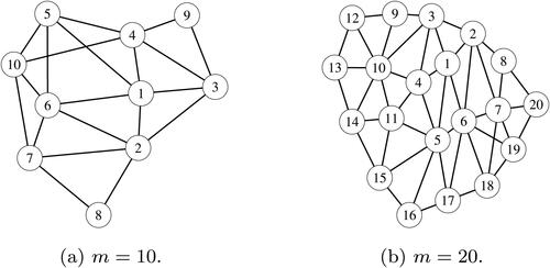
The number of groups is m = 10, 20, the correlation between explanatory variables is $\rho =0.5,$ 0.8, and the sample sizes of groups are $n_1=\cdots =n_m=n_0.$ Then, total sample size is $n=m{n}_0$ and we use $n_0=100,200,500,1000.$ Figure 1 shows simulation groups when m = 10, 20 with adjacent relationships indicated by lines. The figure means, for example, $D_1=\{2,3,4,5,6\}$ and $D_2=\{1,3,6,7,8\}$ when m = 10. We generated data from the simulation model $N_n(\mathit{X\beta }+\mathit{R\mu },{\mathit{I}}_n)$ with the following $\mathit{X}$: $$\mathit{X}=({\mathit{a}}_1,\dots ,{\mathit{a}}_8,{\mathit{A}}_9,\dots ,{\mathit{A}}_{13}),$$ where column vectors ${\mathit{a}}_1,\dots ,{\mathit{a}}_8$ and block matrices ${\mathit{A}}_9,\dots ,{\mathit{A}}_{13}$ are calculated as using the following procedure. Let ${\mathit{u}}_1,\dots ,{\mathit{u}}_{14}$ be independent n-dimensional vectors that the elements are identically and independently distributed according to U(0, 1) and ${\mathit{v}}_1,\dots ,{\mathit{v}}_{13}$ be n-dimensional vectors defined by $${\mathit{v}}_j=\omega {\mathit{u}}_{14}+(1-\omega ){\mathit{u}}_j,$$ where ω is the parameter determining the correlation of ${\mathit{v}}_i$ and ${\mathit{v}}_j(i\ne j)$ as ρ, defined by $$\omega =\{\begin{array}{cc}\frac{\rho \pm \sqrt{{\rho }^2-\rho (2\rho -1)}}{2\rho -1}\hfill & (\rho \ne 1/2)\hfill \\ \frac{1}{2}\hfill & (\rho =1/2)\hfill \end{array}.$$

Figure 1. Simulation groups and adjacent relationship. (a) m = 10. (b) m = 20.

By using these vectors ${\mathit{v}}_1,\dots ,{\mathit{v}}_{13},$ we define the blocks in $\mathit{X}$ as follows: Let ${\mathit{a}}_j={\mathit{v}}_j$ for $j=1,\dots ,5;$ let ${\mathit{a}}_j(j=6,7,8)$ be dummy variables that take the value 1 or 0 defined by $$a_{j,i}=\{\begin{array}{cc}1\hfill & (v_{j,i}>0.6)\hfill \\ 0\hfill & (v_{j,i}\le 0.6)\hfill \end{array}\hspace{1em}\left(i\in \{1,\dots ,n\}\right);$$ and let ${\mathit{A}}_j(j=9,\dots ,13)$ be $(j-7)$-dimensional dummy variables that are categorized, defined by $$(\text{The\hspace{0.5em}}i\text{th\hspace{0.5em}row\hspace{0.5em}vector\hspace{0.5em}of\hspace{0.5em}}{\mathit{A}}_j)=\{\begin{array}{cc}{\mathit{e}}_{\mathit{j}-7,\mathcal{\ell }}\hfill & ({\mathit{v}}_{\mathit{j},\mathit{i}}\in {\mathit{Q}}_{\mathit{j}-6,\mathcal{\ell }},\mathcal{\ell }\ne \mathit{j}-6)\hfill \\ {\mathit{0}}_{\mathit{j}-7}\hfill & ({\mathit{v}}_{\mathit{j},\mathit{i}}\in {\mathit{Q}}_{\mathit{j}-6,\mathit{j}-6})\hfill \end{array}\hspace{1em}(\mathit{i}=1,\dots ,\mathit{n}),$$ where ${\mathit{e}}_{j,\mathcal{\ell }}$ is a j-dimensional vector in which the $\mathcal{\ell }$th element is 1 and the others are 0 and $Q_{j,\mathcal{\ell }}$ is the $\mathcal{\ell }$ th range when $[0,1]$ is split into j ranges. The following 2 cases are used as $\mathit{\beta }$ and $\mathit{\mu }.$

• Case 1: Let the number of true explanatory variables be $k_{\ast }=9$ and the number of true joins of groups be

$$m_{\ast }=\{\begin{array}{cc}3\hfill & (m=10)\hfill \\ 6\hfill & (m=20)\hfill \end{array},$$

and we use the following $\mathit{\beta }$ and $\mathit{\mu }$: $$\mathit{\beta }=\left(1,2,3,0,0,1,1,2,{\mathit{1}}_2^{\prime },{\mathit{0}}_3^{\prime },2\times {\mathit{1}}_4^{\prime },{\mathit{0}}_5^{\prime },3\times {\mathit{1}}_6^{\prime }\right)\prime ,$$ $$\forall j\in E_{\mathcal{\ell }},{\mu }_j=\mathcal{\ell }\hspace{1em}(\mathcal{\ell }=1,\dots ,m_{\ast }).$$

• Case 2: Let the number of true explanatory variables be $k_{\ast }=3$ and the number of true joins of groups be

$$m_{\ast }=\{\begin{array}{cc}6\hfill & (m=10)\hfill \\ 12\hfill & (m=20)\hfill \end{array},$$

and we use the following $\mathit{\beta }$ and $\mathit{\mu }$: $$\begin{array}{c}\mathit{\beta }=\left(1,0,0,0,0,1,0,0,{\mathit{0}}_2^{\prime },{\mathit{0}}_3^{\prime },2\times {\mathit{1}}_4^{\prime },{\mathit{0}}_5^{\prime },{\mathit{0}}_6^{\prime }\right)\prime ,\\ \forall j\in E_{\mathcal{\ell }},\hspace{0.5em}{\mu }_j=\mathcal{\ell }\hspace{1em}(\mathcal{\ell }=1,\dots ,m_{\ast }).\end{array}$$

Figures 2 and 3 show true joins of groups when m = 10, 20, respectively. Estimation accuracy is evaluated by the selection probabilities of true variables and true joins by Monte Carlo simulation with 1000 iterations. Tables 1 and 2 show the selection probabilities (SP) of true variables and true joins and running times (RT) of programs in Cases 1 and 2, respectively. The SP is displayed as the combined probability (C-SP) and separate probability about variables and joins. From the tables, since the SP of Method 1 approaches 100% as sample size increases, we found that Method 1 has high estimation accuracy. On the other hand, Method 2 struggles to select the true variables and true joins and its SP is 7.4% (when m = 10, $\rho =0.8,$ and $n=5000$ in Case 1) at most. In particular, it struggles to select the true joins and its SP is only 7.8% (when m = 10, $\rho =0.8,$ and $n=5000$ in Case 1) at most. Moreover, in terms of running time, Method 1 is about 134 times faster than Method 2 (when m = 20, $\rho =0.5,$ and $n=20,000$ in Case 1) at most.

Figure 2. True joins when m = 10. (a) Case 1. (b) Case 2.

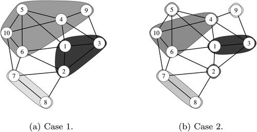
Figure 3. True joins when m = 20. (a) Case 1. (b) Case 2.

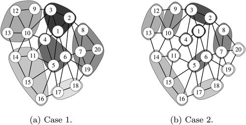
Table 1. Selection probabilities and running times in Case 1.

			Method 1				Method 2
m	Ρ	n	C-SP	SP ($\mathit{\beta }$)	SP ($\mathit{\mu }$)	RT (s)	C-SP	SP ($\mathit{\beta }$)	SP ($\mathit{\mu }$)	RT (s)
10	0.5	1000	74.20	92.40	79.90	0.65	4.30	92.10	5.00	0.39
		2000	88.60	97.60	91.00	0.60	4.10	97.60	4.10	0.68
		5000	93.80	98.50	95.20	0.58	6.00	98.50	6.10	4.14
		10,000	95.00	97.30	97.60	0.64	3.90	97.30	4.00	14.27
	0.8	1000	59.60	73.70	79.90	1.01	3.20	73.60	5.10	0.53
		2000	82.60	92.40	89.90	0.86	4.80	92.20	5.20	0.91
		5000	91.40	95.40	95.80	0.82	7.40	95.40	7.80	4.68
		10,000	93.20	95.30	97.90	0.67	3.70	95.30	3.80	14.70
20	0.5	2000	72.70	98.60	73.80	1.21	0.00	98.60	0.00	1.48
		4000	85.20	98.80	86.30	1.23	0.00	98.70	0.00	6.14
		10,000	93.80	99.10	94.70	1.22	0.00	99.00	0.00	27.01
		20,000	97.60	98.90	98.70	1.10	0.10	98.90	0.10	148.04
	0.8	2000	69.20	92.90	74.40	1.60	0.30	92.90	0.30	1.77
		4000	83.30	95.90	86.80	1.47	0.00	96.00	0.00	6.63
		10,000	90.00	95.30	94.30	1.23	0.10	95.40	0.10	29.64
		20,000	94.10	95.30	98.70	1.18	0.00	95.40	0.00	146.24

Table 2. Selection probabilities and running times in Case 2.

			Method 1				Method 2
M	Ρ	n	C-SP	SP ($\mathit{\beta }$)	SP ($\mathit{\mu }$)	RT (s)	C-SP	SP ($\mathit{\beta }$)	SP ($\mathit{\mu }$)	RT (s)
10	0.5	1000	74.00	91.60	81.20	1.39	2.90	91.20	3.20	0.41
		2000	87.30	97.20	89.90	0.84	0.90	97.10	0.90	0.52
		5000	94.80	98.80	95.90	0.76	4.50	98.80	4.50	3.15
		10,000	95.90	98.50	97.30	0.71	1.40	98.40	1.40	11.41
	0.8	1000	55.10	69.10	80.30	2.35	1.80	69.20	2.80	0.66
		2000	81.20	91.30	89.40	1.05	1.80	91.50	2.00	0.61
		5000	92.40	96.00	96.10	0.81	2.80	96.00	2.80	3.24
		10,000	94.10	96.60	97.40	0.87	2.20	96.60	2.30	12.62
20	0.5	2000	63.40	97.90	65.00	1.53	0.10	97.90	0.10	1.06
		4000	80.90	98.50	81.90	1.37	0.00	98.60	0.00	3.97
		10,000	92.70	99.20	93.40	1.32	0.40	99.20	0.40	20.63
		20,000	96.40	99.30	97.10	1.32	0.10	99.40	0.10	144.11
	0.8	2000	59.60	91.20	66.20	1.77	0.30	91.20	0.30	1.20
		4000	80.10	96.70	82.80	1.43	0.00	96.60	0.00	4.38
		10,000	90.70	97.00	93.50	1.47	0.70	97.00	0.70	27.11
		20,000	94.80	97.50	97.10	1.41	0.00	97.60	0.00	148.19

3.2. A real data example

In this subsection, we present an illustrative application of the proposed method (Method 1 in Subsection 3.1) to an actual data set. Actually, Method 2 in Subsection 3.1 cannot run the program because the genlasso package causes memory shortage since the applied data have a large sample. This is the motivation of this paper. The data pertain to studio apartment rents and environmental conditions in Tokyo’s 23 wards collected by Tokyo Kantei Co., Ltd. Here, $n=61,999$ and all data were collected between April 2014 and April 2015 (Table 3). In this application, let the response variable be monthly rent with the remainder set as explanatory variables. We estimate regional effects at 852 areas split Tokyo’s 23 wards using the proposed method. Figure 4 shows the split of Tokyo’s 23 wards into 852 areas. Figure 5 shows estimates and clustering result of regional effects in the form of choropleth map. In terms of the former, as with Figure 5b, the 852 areas in Tokyo’s 23 wards are clustered to form 190 areas. Table 4 summarizes estimates of regression coefficients. As a result of variable selection, B5 and C1 are not selected. Figure 6 is residual plots for quantitative variables. Table 5 provides information concerning coefficients of determination (R²), median error rate (MER), and running time. From the results, R² is more than 0.8, MER is less than 10%, and the residual plots are unproblematic. Thus, the proposed method performs well. In this application, we have applied the CDA for GFL to large sample data. For such data, the genlasso package caused memory shortage. Nevertheless the CDA completed program in only about 2 minutes. This is our big contribution.

Figure 4. The 852 areas in Tokyo’s 23 wards.

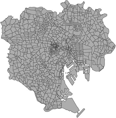
Figure 5. Regional effects estimation results. (a) Estimates. (b) Clustering.

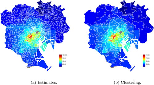
Figure 6. Residual plots. (a) Floor area (A). (b) Age (C3). (c) Interaction (C4). (d) Walking time (C5).

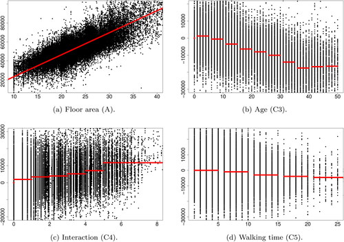
Table 3. Data items.

Y	Monthly rent of an apartment (yen)
A	Floor area of an apartment (m^2)
B1	Whether an apartment has a parking lot
B2	Whether an apartment is a condominium
B3	Whether an apartment is a corner apartment
B4	Whether an apartment is a fixed-term tenancy agreement
B5	Whether an apartment is on the top floor
C1	Facing direction
	base: South	C1a: North	C1b: Northeast
	C1c: East	C1d: Southeast	C1e: Southwest
	C1f: West	C1g: Northwest
C2	Building structure
	base: Reinforced concrete	C2a: Wooden	C2b: Light steel frame
	C2c: Steel frame	C2d: Steel framed rein-forced concrete	C2e: ALC
	C2f: Steel framed precast concrete	C2g: Precast concrete	C2h: Reinforced block
	C2i: Other
C3	Building age (years)
	base: 0 (new-build)	C3a: 1–5	C3b: 6–10
	C3c: 11–15	C3d: 16–20	C3e: 21–25
	C3f: 26–30	C3g: 31–35	C3h: 36–40
	C3i: 41–45	C3j: 46–50
C4	Interaction of logarithmic transformations of the top floor and a room floor
	base: 0	C4a: 0–1	C4b: 1–2
	C4c: 2–3	C4d: 3–4	C4e: 4–5
	C4f: $5<$
C5	Walking time (min) to the nearest station
	base: 1–5	C5a: 6–10	C5b: 11–15
	C5c: 16–20	C5d: $21\le$

Y and A are continuous variables. B1 to B5 are dummy variables that take the value of 1 or 0. C1 to C5 are multidimensional dummy variables. C3 to C5 were transformed from continuous variables to categorical variables.

Table 4. Regression coefficient estimates.

A	0.67942	C2b	−0.01053	C3g	−0.04101
B1	0.00666	C2c	−0.00844	C3h	−0.03809
B2	−0.00925	C2d	−0.00675	C3i	−0.03330
B3	−0.00954	C2e	−0.00689	C3j	−0.02307
B4	0.00468	C2f	−0.00016	C4a	0.01151
B5	0	C2g	−0.00211	C4b	0.02015
C1a	0	C2h	−0.00012	C4c	0.01583
C1b	0	C2i	−0.00297	C4d	0.01803
C1c	0	C3a	0.00596	C4e	0.02212
C1d	0	C3b	−0.00286	C4f	0.03702
C1e	0	C3c	−0.01729	C5a	−0.00774
C1f	0	C3d	−0.02185	C5b	−0.01239
C1g	0	C3e	−0.03560	C5c	−0.00708
C2a	−0.01291	C3f	−0.04550	C5d	−0.00422

Table 5. Model fit and run time.

R^2	MER (%)	Run time (min)
0.835	6.720	2.406

4. Conclusion

In this paper, we challenged a coordinate optimization for GFL and derived the update equations for descent cycle and fusion cycle as closed forms, respectively. The update equations can be obtained by only using fundamental mathematics and some complex conditions (e.g., the Karush-Kuhn-Tucker conditions) are not required. In the numerical studies, we found that our proposed method gives accurate solution rapidly than existing method (which is using the genlasso package) and can be applied to even a large sample data that the genlasso package causes memory shortage.

Here, our proposed method was obtained for a linear regression model. However, the method can be also applied to models which are not linear. For example, for generalized linear models, by approximating a negative logarithm likelihood function by a linear function, the GFL-penalized objective function has equal class to (3)(3) $$\Vert \tilde{\mathit{y}}-\mathit{R\mu }{\Vert }_2^2+\lambda \sum _{j=1}^m\sum _{\mathcal{\ell }\in D_j}{w}_{j\mathcal{\ell }}|{\mu }_j-{\mu }_{\mathcal{\ell }}|,$$(3) . That is our proposed method can be applied to even generalized linear models. On the other hand, the method cannot work for an extension of GFL penalty. For example, when group-GFL penalty is used instead of GFL penalty (it means the case that μ_j is a vector), the method cannot be applied.

Acknowledgments

The authors thank Dr. Ryoya Oda and Mr. Yuya Suzuki of Hiroshima University, Mr. Yuhei Sato and Mr. Yu Matsumura of Tokyo Kantei Co., Ltd., and Koki Kirishima of Computer Management Co., Ltd., for helpful comments. Moreover, the authors also thank the associate editor and the reviewers for their valuable comments.

Additional information

Funding

The first author’s research was partially supported by JSPS KAKENHI Grant Numbers JP20H04151 and JP21K13834. The second author’s research was partially supported by JSPS KAKENHI Grant Numbers JP17K15842, JP18K10068, JP19H01076, JP20H04151, and JP21K17288. The last author’s research was partially supported by JSPS KAKENHI Grant Numbers JP18K03415 and JP20H0415.

Appendix A. Proof of Lemma 2.1

We partition (3)(3) $$\Vert \tilde{\mathit{y}}-\mathit{R\mu }{\Vert }_2^2+\lambda \sum _{j=1}^m\sum _{\mathcal{\ell }\in D_j}{w}_{j\mathcal{\ell }}|{\mu }_j-{\mu }_{\mathcal{\ell }}|,$$(3) into terms that do and do not depend on μ_i. The first term in (3)(3) $$\Vert \tilde{\mathit{y}}-\mathit{R\mu }{\Vert }_2^2+\lambda \sum _{j=1}^m\sum _{\mathcal{\ell }\in D_j}{w}_{j\mathcal{\ell }}|{\mu }_j-{\mu }_{\mathcal{\ell }}|,$$(3) can be partitioned as follows: (A1) $$\begin{array}{c}\Vert \tilde{\mathit{y}}-\mathit{R\mu }{\Vert }_2^2=\Vert \tilde{\mathit{y}}{\Vert }_2^2-2\tilde{\mathit{y}}\prime \mathit{R\mu }+\mathit{\mu }\prime \mathit{R}\prime \mathit{R\mu }\\ =\Vert \tilde{\mathit{y}}{\Vert }_2^2-2\left(\sum _{j\ne i}^m{\widehat{\mu }}_j{\tilde{\mathit{y}}}_j^{\prime }{\mathit{1}}_{n_j}+{\mu }_i{\tilde{\mathit{y}}}_i^{\prime }{\mathit{1}}_{n_i}\right)+\sum _{j\ne i}^m{n}_j{\widehat{\mu }}_j^2+n_i{\mu }_i^2\\ =n_i{\mu }_i^2-2{\tilde{\mathit{y}}}_i^{\prime }{\mathit{1}}_{n_i}{\mu }_i+\sum _{j\ne i}^m(n_j{\widehat{\mu }}_j^2-2{\tilde{\mathit{y}}}_j^{\prime }{\mathit{1}}_{n_j}{\widehat{\mu }}_j)+\Vert \tilde{\mathit{y}}{\Vert }_2^2.\end{array}$$(A1)

Moreover, since $w_{j\mathcal{\ell }}=w_{\mathcal{\ell }j},$ the second term in (3)(3) $$\Vert \tilde{\mathit{y}}-\mathit{R\mu }{\Vert }_2^2+\lambda \sum _{j=1}^m\sum _{\mathcal{\ell }\in D_j}{w}_{j\mathcal{\ell }}|{\mu }_j-{\mu }_{\mathcal{\ell }}|,$$(3) can be partitioned as follows: $$\begin{array}{c}\sum _{j=1}^m\sum _{\mathcal{\ell }\in D_j}{w}_{j\mathcal{\ell }}|{\mu }_j-{\mu }_{\mathcal{\ell }}|=\sum _{j\ne i}^m\sum _{\mathcal{\ell }\in D_j}{w}_{j\mathcal{\ell }}|{\mu }_j-{\mu }_{\mathcal{\ell }}|+\sum _{\mathcal{\ell }\in D_i}{w}_{i\mathcal{\ell }}|{\mu }_i-{\mu }_{\mathcal{\ell }}|\\ =\sum _{j\ne i}^m\sum _{\mathcal{\ell }\in \underset{j}{D}}i{w}_{j\mathcal{\ell }}|{\widehat{\mu }}_j-{\widehat{\mu }}_{\mathcal{\ell }}|+2\sum _{\mathcal{\ell }\in D_i}{w}_{i\mathcal{\ell }}|{\mu }_i-{\widehat{\mu }}_{\mathcal{\ell }}|.\end{array}$$

Consequently, Lemma 2.1 is proved, where u_i is given by $$u_i=\sum _{j\ne i}^m(n_j{\widehat{\mu }}_j^2-2{\tilde{\mathit{y}}}_j^{\prime }{\mathit{1}}_{n_j}{\widehat{\mu }}_j)+\Vert \tilde{\mathit{y}}{\Vert }_2^2+{\lambda }_2\sum _{j\ne i}^m\sum _{\mathcal{\ell }\in \underset{j}{D}}i{w}_{2,j\mathcal{\ell }}|{\widehat{\mu }}_j-{\widehat{\mu }}_{\mathcal{\ell }}|.$$

Appendix B. Proof of Theorem 2.2

First, we rewrite (5)(5) $$\varphi (x)=c_2{x}^2-2c_{1}x+2\lambda \sum _{j=1}^r{w}_j|x-b_j|\hspace{1em}(c_2,w_1,\dots ,w_r>0).$$(5) in non absolute form. Since $t_1,\dots ,t_r$ are the order statistics of $b_1,\dots ,b_r,$ the following equation holds when $x\in R_a:$ $$\begin{array}{c}\sum _{j=1}^r{w}_j|x-b_j|=\sum _{j\in J_a^{+}}{w}_j(x-b_j)+\sum _{j\in J_a^{-}}{w}_j(b_j-x)\\ ={\tilde{w}}_{a}x-\left(\sum _{j\in J_a^{+}}{w}_j{b}_j-\sum _{j\in J_a^{-}}{w}_j{b}_j\right).\end{array}$$

Thus, we have the following non absolute form of (5)(5) $$\varphi (x)=c_2{x}^2-2c_{1}x+2\lambda \sum _{j=1}^r{w}_j|x-b_j|\hspace{1em}(c_2,w_1,\dots ,w_r>0).$$(5) : $$\varphi (x)={\varphi }_a(x)=c_2{x}^2-2(c_1-\lambda {\tilde{w}}_a)x-2\lambda \left(\sum _{j\in J_a^{+}}{w}_j{b}_j-\sum _{j\in J_a^{-}}{w}_j{b}_j\right)\hspace{1em}(x\in R_a;a=0,1,\dots ,r).$$

From the above equation, we found that v_a is the x-coordinate of the vertex of the quadratic function ${\varphi }_a(x)$ and the minimizer of $\varphi (x)$ is included in $\{v_0,v_1,\dots ,v_r,t_1,\dots ,t_r\}$. The piecewise function $\varphi (x)={\varphi }_a(x)(x\in R_a)$ has the following properties (the proof is given in Appendix D.1):

Lemma B.1.

The $\varphi (x)$ is continuous in $x\in \mathbb{R}$, that is, ${\varphi }_a(t_{a+1})={\varphi }_{a+1}(t_{a+1})(a=0,1,\dots ,r-1)$ and v_a is a monotonically decreasing sequence with respect to a.

From this lemma, we have the following lemma (the proof is given in Appendix D.2):

Lemma B.2.

Let $a^{\ast }$ and $a^{\star }$ be non negative values defined by $$a^{\ast }\in \{0,1,\dots ,r\}s.t.v_{a^{\ast }}\in R_{a^{\ast }},\hspace{1em}{a}^{\star }\in \{1,\dots ,r\}s.t.t_{a^{\star }}\in [v_{a^{\star }},v_{a^{\star }-1}).$$

Then, either $a^{\ast }$ or $a^{\star }$ uniquely exists.

Lemma B.2 says that existing $v_{a^{\ast }}$ or $t_{a^{\star }}$ is a local minimizer. In addition, because $\varphi (x)$ is a continuous function, the local minimizer is the minimizer of $\varphi (x).$ Consequently, Theorem 2.2 is proved.

Appendix C. Proof of Lemma 2.3

From (1)(1) $${\mathit{y}}_j={\mathit{X}}_j\mathit{\beta }+{\mu }_j{\mathit{1}}_{n_j}+{\mathit{\epsilon }}_j,$$(1) , we have $$\Vert \tilde{\mathit{y}}-\mathit{R\mu }{\Vert }_2^2=\sum _{j\in E_i}{n}_j{\eta }_i^2-2\sum _{j\in E_i}{\tilde{\mathit{y}}}_j\prime {\mathit{1}}_{n_j}{\eta }_i+\sum _{j\notin E_i}(n_j{\widehat{\mu }}_j^2-2{\tilde{\mathit{y}}}_j^{\prime }{\mathit{1}}_{n_j}{\widehat{\mu }}_j)+\Vert \tilde{\mathit{y}}{\Vert }_2^2.$$

Moreover, the second term in (3)(3) $$\Vert \tilde{\mathit{y}}-\mathit{R\mu }{\Vert }_2^2+\lambda \sum _{j=1}^m\sum _{\mathcal{\ell }\in D_j}{w}_{j\mathcal{\ell }}|{\mu }_j-{\mu }_{\mathcal{\ell }}|,$$(3) can be partitioned as follows: $$\begin{array}{c}\sum _{j=1}^m\sum _{\mathcal{\ell }\in D_j}{w}_{j\mathcal{\ell }}|{\mu }_j-{\mu }_{\mathcal{\ell \ell }}|=\sum _{j\notin E_i}\sum _{\mathcal{\ell }\in D_j}{w}_{j\mathcal{\ell }}|{\mu }_j-{\mu }_{\mathcal{\ell }}|+\sum _{j\in E_i}\sum _{\mathcal{\ell }\in D_j}{w}_{j\mathcal{\ell }}|{\mu }_j-{\mu }_{\mathcal{\ell }}|\\ =\sum _{j\notin E_i}\sum _{\mathcal{\ell }\in D_j{E}_i}{w}_{j\mathcal{\ell }}|{\widehat{\mu }}_j-{\widehat{\mu }}_{\mathcal{\ell }}|+\sum _{j\notin E_i}\sum _{\mathcal{\ell }\in D_j\cap E_i}{w}_{j\mathcal{\ell }}|{\widehat{\mu }}_j-{\mu }_{\mathcal{\ell }}|\\ \mathrm{\hspace{1em}}\mathrm{\hspace{1em}}+\sum _{j\in E_i}\sum _{\mathcal{\ell }\in D_j{E}_i}{w}_{j\mathcal{\ell }}|{\mu }_j-{\widehat{\mu }}_{\mathcal{\ell }}|+\sum _{j\in E_i}\sum _{\mathcal{\ell }\in D_j\cap E_i}{w}_{j\mathcal{\ell }}|{\mu }_j-{\mu }_{\mathcal{\ell }}|\\ =\sum _{j\notin E_i}\sum _{\mathcal{\ell }\in D_j{E}_i}{w}_{j\mathcal{\ell }}|{\widehat{\mu }}_j-{\widehat{\mu }}_{\mathcal{\ell }}|+\sum _{j\notin E_i}\sum _{\mathcal{\ell }\in D_j\cap E_i}{w}_{j\mathcal{\ell }}|{\widehat{\mu }}_j-{\eta }_i|\\ \mathrm{\hspace{1em}}\mathrm{\hspace{1em}}+\sum _{j\in E_i}\sum _{\mathcal{\ell }\in D_j{E}_i}{w}_{j\mathcal{\ell }}|{\eta }_i-{\widehat{\mu }}_{\mathcal{\ell }}|+\sum _{j\in E_i}\sum _{\mathcal{\ell }\in D_j\cap E_i}{w}_{j\mathcal{\ell }}|{\eta }_i-{\eta }_i|\\ =\sum _{j\notin E_i}\sum _{\mathcal{\ell }\in D_j{E}_i}{w}_{j\mathcal{\ell }}|{\widehat{\mu }}_j-{\widehat{\mu }}_{\mathcal{\ell }}|+2\sum _{j\in E_i}\sum _{\mathcal{\ell }\in D_j{E}_i}{w}_{j\mathcal{\ell }}|{\eta }_i-{\widehat{\mu }}_{\mathcal{\ell }}|.\end{array}$$

All pairs $(j,\mathcal{\ell })$ in the second term of the above equation are expressed as the following set: $$\underset{j\in E_i}{\cup }\left\{j\right\}\times (D_j\backslash E_i).$$

Regarding this set, we have the following lemma (the proof is given in Appendix D.3):

Lemma C.1.

The following two sets are equal: $$\underset{j\in E_i}{\cup }\left\{j\right\}\times (D_j\backslash E_i)=\underset{\mathcal{\ell }\in D_i^{\ast }}{\cup }{\mathcal{J}}_{i\mathcal{\ell }}.$$

This lemma gives that $$\sum _{j\in E_i}\sum _{\mathcal{\ell }\in D_j\backslash E_i}{w}_{j\mathcal{\ell }}|{\eta }_i-{\widehat{\mu }}_{\mathcal{\ell }}|=\sum _{\mathcal{\ell }\in D_i^{\ast }}\sum _{(j,s)\in {\mathcal{J}}_{i\mathcal{\ell }}}{w}_{js}|{\eta }_i-{\widehat{\mu }}_s|=\sum _{\mathcal{\ell }\in D_i^{\ast }}{w}_{i\mathcal{\ell }}^{\ast }|{\eta }_i-{\widehat{\eta }}_{\mathcal{\ell }}|.$$

Consequently, Lemma 2.3 is proved, where $u_i^{\ast }$ is given by $$u_i^{\ast }=\sum _{j\notin E_i}(n_j{\widehat{\mu }}_j^2-2{\tilde{\mathit{y}}}_j^{\prime }{\mathit{1}}_{n_j}{\widehat{\mu }}_j)+\Vert \tilde{\mathit{y}}{\Vert }_2^2+\lambda \sum _{j\notin E_i}\sum _{\mathcal{\ell }\in D_j\backslash E_i}{w}_{j\mathcal{\ell }}|{\widehat{\mu }}_j-{\widehat{\mu }}_{\mathcal{\ell }}|.$$

Appendix D. Proof of lemmas in appendix

Proof of Lemma B.1

First, we prove that v_a is a monotonically decreasing sequence. The following equation holds: $${\tilde{w}}_a=\sum _{j\in J_a^{+}}{w}_j-\sum _{j\in J_a^{-}}{w}_j=\left(\sum _{j\in J_{a+1}^{+}}{w}_j-w_{j_{\ast }}\right)-\left(\sum _{j\in J_{a+1}^{-}}{w}_j+w_{j_{\ast }}\right)={\tilde{w}}_{a+1}-2w_{j_{\ast }},$$ where $j_{\ast }=\mathrm{arg\hspace{0.17em}}{\min }_{j\in J_a^{-}}{b}_j=\mathrm{arg\hspace{0.17em}}{\max }_{j\in J_{a+1}^{+}}{b}_j.$ Since $w_j>0,{\tilde{w}}_a$ is a monotonically increasing sequence with respect to a. Thus, v_a is a monotonically decreasing sequence with respect to a.

Next, we prove that $\varphi (x)$ is a continuous function. The following equation holds about the term of ${\varphi }_a(t_{a+1})$ that depends on a: $$\begin{array}{c}2\lambda {\tilde{w}}_a{t}_{a+1}-2\lambda \left(\sum _{j\in J_a^{+}}{w}_j{b}_j-\sum _{j\in J_a^{-}}{w}_j{b}_j\right)\\ =2\lambda {\tilde{w}}_{a+1}{t}_{a+1}-4\lambda w_{j_{\ast }}{t}_{a+1}-2\lambda \left(\sum _{j\in J_{a+1}^{+}}{w}_j{b}_j-\sum _{j\in J_{a+1}^{-}}{w}_j{b}_j-2w_{j_{\ast }}{t}_{a+1}\right)\\ =2\lambda {\tilde{w}}_{a+1}{t}_{a+1}-2\lambda \left(\sum _{j\in J_{a+1}^{+}}{w}_j{b}_j-\sum _{j\in J_{a+1}^{-}}{w}_j{b}_j\right).\end{array}$$

Thus, we have ${\varphi }_a(t_{a+1})={\varphi }_{a+1}(t_{a+1}).$

Consequently, Lemma B.1 is proved.

Proof of Lemma B.2

The following statement is true: $$\begin{array}{c}{a}^{\star }\text{\hspace{0.5em}does}\mathrm{ }\text{not}\mathrm{ }\text{exist}\iff \forall a\in \{1,\dots ,r\},t_a\notin [v_a,v_{a-1})\\ \iff \{\begin{array}{c}\forall a\in \{1,\dots ,r\},v_{a-1}\le t_a\hfill \\ \forall a\in \{1,\dots ,r\},t_a<v_a\hfill \\ \exists !a_0\in \{1,\dots ,r-1\}s.t.\{\begin{array}{cc}{t}_a<v_{a_0}\hfill & (a\le a_0-1)\hfill \\ v_{a_0}\le t_a\hfill & (a_0\le a)\hfill \end{array}\hfill \end{array}\\ \iff \{\begin{array}{cc}{v}_0\in R_0\hfill & (a^{\ast }=0)\hfill \\ v_r\in R_r\hfill & (a^{\ast }=r)\hfill \\ v_{a_0}\in R_{a_0}\hfill & (a^{\ast }=a_0\in \{1,\dots ,r-1\})\hfill \end{array}\\ \iff \exists a^{\ast }\in \{0,1,\dots ,r\}s.t.v_{a^{\ast }}\in R_{a^{\ast }}\\ \iff a^{\ast }\text{exists}.\end{array}$$

The fact says that only either $a^{\ast }$ or $a^{\star }$ exists.

Regarding the uniqueness of $a^{\ast },$ assume that $a_1(\in \{0,1,\dots ,r\})$ and $a_2(\in \{0,1,\dots ,r\})$ exist such that $v_{a_1}\in R_{a_1}$ and $v_{a_2}\in R_{a_2},$ and they satisfy $a_1+1\le a_2$ without loss of generality. Then, although $t_{a_1}<v_{a_1}\le t_{a_1+1}\le t_{a_2}<v_{a_2}\le t_{a_2+1}$ holds, this is in conflict with $v_{a_2}<v_{a_1}.$ Thus, we have a₁ = a₂.

Regarding the uniqueness of $a^{\star },$ assume that $a_1(\in \{1,\dots ,r\})$ and $a_2(\in \{1,\dots ,r\})$ exist such that $t_{a_1}\in [v_{a_1},v_{a_1-1})$ and $t_{a_2}\in [v_{a_2},v_{a_2-1})$ and they satisfy $a_1+1\le a_2$ without loss of generality. Then, although $v_{a_1}\le t_{a_1}\le t_{a_2}<v_{a_2-1}$ holds, this is in conflict with $v_{a_2-1}\le v_{a_1}.$ Thus, we have a₁ = a₂.

Consequently, Lemma B.2 is proved.

Proof of Lemma C.1

First, we show that $$\underset{j\in E_i}{\cup }\left\{j\right\}\times (D_j\backslash E_i)\subset \underset{\mathcal{\ell }\in D_i^{\ast }}{\cup }{\mathcal{J}}_{i\mathcal{\ell }}.$$

Let $(\mathcal{\ell },s)$ be an element of the above LHS. Then, the following statement is true: $$\begin{array}{c}(\mathcal{\ell },s)\in \underset{j\in E_i}{\cup }\left\{j\right\}\times (D_j\backslash E_i)\iff \exists j_0\in E_{i}s.t.(\mathcal{\ell },s)\in \left\{j_0\right\}\times (D_{j_0}\backslash E_i)\\ \iff \exists j_0\in E_{i}s.t.\mathcal{\ell }=j_0\wedge s\in D_{j_0}\backslash E_i.\end{array}$$

The $s\in D_{j_0}\backslash E_i$ leads $s\in F_i$ and $$s\in D_{j_0}\wedge s\notin E_i\iff s\in D_{j_0}\wedge \exists !{\mathcal{\ell }}_0\in \{1,\dots ,b\}\backslash \left\{i\right\}s.t.s\in E_{{\mathcal{\ell }}_0}.$$

These results say $s\in E_{{\mathcal{\ell }}_0}\cap F_i$ and hence ${\mathcal{\ell }}_0\in D_i^{\ast }.$ Notice that $(\mathcal{\ell },s)\in \left\{j_0\right\}\times E_{{\mathcal{\ell }}_0}\cap D_{j_0}.$ Hence, we have $$(\mathcal{\ell },s)\in \underset{\mathcal{\ell }\in D_i^{\ast }}{\cup }{\mathcal{J}}_{i\mathcal{\ell }}.$$

Next, we show that $$\underset{j\in E_i}{\cup }\left\{j\right\}\times (D_j\backslash E_i)\supset \underset{\mathcal{\ell }\in D_i^{\ast }}{\cup }{\mathcal{J}}_{i\mathcal{\ell }}.$$

Let $(\mathcal{\ell },s)$ be an element of the above RHS. Then, the following statement is true: $$\begin{array}{c}(\mathcal{\ell },s)\in \underset{\mathcal{\ell }\in D_i^{\ast }}{\cup }{\mathcal{J}}_{i\mathcal{\ell }}\iff \exists {\mathcal{\ell }}_0\in D_i^{\ast }s.t.\left(\exists j_0\in E_{i}s.t.(\mathcal{\ell },s)\in \left\{j_0\right\}\times E_{{\mathcal{\ell }}_0}\cap D_{j_0}\right)\\ \Rightarrow \mathcal{\ell }=j_0\wedge s\in E_{{\mathcal{\ell }}_0}\times D_{j_0}.\end{array}$$

Moreover, we found that $s\notin E_i$ because ${\mathcal{\ell }}_0\in D_i^{\ast }.$ Hence, we have $$(\mathcal{\ell },s)\in \underset{j\in E_i}{\cup }\left\{j\right\}\times (D_j\backslash E_i).$$

Consequently, Lemma C.1 is proved.

References

- Arnold, T., and R. Tibshirani. 2019. genlasso: Path Algorithm for Generalized Lasso Problems. R package version 1.4. https://CRAN.R-project.org/package=genlasso.
- Donoho, D. L., and I. M. Johnstone. 1994. Ideal spatial adaptation by wavelet shrinkage. Biometrika 81 (3):425–55. doi: https://doi.org/10.1093/biomet/81.3.425.
- Friedman, J., T. Hastie, H. Höfling, and R. Tibshirani. 2007. Pathwise coordinate optimization. The Annals of Applied Statistics 1 (2):302–32. doi: https://doi.org/10.1214/07-AOAS131.
- Li, F., and H. Sang. 2019. Spatial homogeneity pursuit of regression coefficients for large datasets. Journal of the American Statistical Association 114 (527):1050–62. doi: https://doi.org/10.1080/01621459.2018.1529595.
- Ohishi, M., H. Yanagihara, and Y. Fujikoshi. 2020. A fast algorithm for optimizing ridge parameters in a generalized ridge regression by minimizing a model selection criterion. Journal of Statistical Planning and Inference 204:187–205. doi: https://doi.org/10.1016/j.jspi.2019.04.010.
- R Core Team. 2019. R: A language and environment for statistical computing. Vienna, Austria: R Foundation for Statistical Computing. https://www.R-project.org/.
- Sun, Y., H. J. Wang, and M. Fuentes. 2016. Fused adaptive Lasso for spatial and temporal quantile function estimation. Technometrics 58 (1):127–37. doi: https://doi.org/10.1080/00401706.2015.1017115.
- Tibshirani, R. 1996. Regression shrinkage and selection via the Lasso. Journal of the Royal Statistical Society: Series B (Methodological) 58 (1):267–88. doi: https://doi.org/10.1111/j.2517-6161.1996.tb02080.x.
- Tibshirani, R., and J. Taylor. 2011. The solution path of the generalized Lasso. The Annals of Statistics 39:1335–71.
- Tibshirani, R., M. Saunders, S. Rosset, J. Zhu, and K. Knight. 2005. Sparsity and smoothness via the fused Lasso. Journal of the Royal Statistical Society: Series B (Statistical Methodology) 67 (1):91–108. doi: https://doi.org/10.1111/j.1467-9868.2005.00490.x.
- Yuan, M., and Y. Lin. 2006. Model selection and estimation in regression with grouped variables. Journal of the Royal Statistical Society: Series B (Statistical Methodology) 68 (1):49–67. doi: https://doi.org/10.1111/j.1467-9868.2005.00532.x.
- Zou, H. 2006. The adaptive Lasso and its oracle properties. Journal of the American Statistical Association 101 (476):1418–29. doi: https://doi.org/10.1198/016214506000000735.